Collisional shifts in optical-lattice atom clocks

Abstract

We theoretically study the effects of elastic collisions on the determination of frequency standards via Ramsey fringe spectroscopy in optical-lattice atom clocks. Interparticle interactions of bosonic atoms in multiply-occupied lattice sites can cause a linear frequency shift, as well as generate asymmetric Ramsey fringe patterns and reduce fringe visibility due to interparticle entanglement. We propose a method of reducing these collisional effects in an optical lattice by introducing a phase difference of $\pi$ between the Ramsey driving fields in adjacent sites. This configuration suppresses site to site hopping due to interference of two tunneling pathways, without degrading fringe visibility. Consequently, the probability of double occupancy is reduced, leading to cancellation of collisional shifts.

I Introduction

Current state-of-the-art atomic clock technology is based mainly on trapped single ions or on clouds of free falling cold atoms clock_reviews . Recently, a new type of atomic clock based on neutral atoms trapped in a deep “magic-wavelength” optical lattice, wherein the ground and excited clock states have equal light shifts, has been suggested Takamoto_03 ; Katori_03 . For interfering, far-detuned light fields, giving rise to a “washboard” intensity pattern, the optical potential experienced by an atom in a given internal state is $V_{0}({\mathbf{r}})=\hbar|\Omega_{0}({\mathbf{r}})|^{2}/(4\Delta_{0})$ where $\Omega_{0}({\mathbf{r}})=2\mu E_{0}({\mathbf{r}})/\hbar$ is the dipole coupling frequency, $E_{0}({\mathbf{r}})$ is the radiation electric field strength at position ${\mathbf{r}}$, and $\Delta_{0}$ is the detuning of the oscillating optical field from resonance. In a magic-wavelength optical lattice, the same exact potential is experienced by the ground and the excited state of the clock transition.

Optical-lattice atomic clocks are advantageous due to the suppression of Doppler shifts by freezing of translational motion (the clock operates in the Lamb-Dicke regime, where atoms are restricted to a length-scale smaller than the transition wavelength Dicke_53 ), the narrow linewidth due to the long lifetime of the states involved in the clock transition, and the large number $M$ of occupied sites, minimizing the Allan standard deviation clock_reviews . As already mentioned, the optical-lattice potential light shift is overcome by using trapping lasers at the magic wavelength Katori_03 ; Takamoto_03 . Operating optical-lattice clocks in the optical frequency regime, rather than in the microwave, has the added benefit of increasing the clock frequency $\nu$ and thereby reducing $\delta\nu/\nu$ by five orders of magnitude. A coherent link between optical frequencies and the microwave cesium standard is provided by the frequency comb method comb . Thanks to these characteristics, atomic optical-lattice clocks have promise of being the frequency standards of the future. Attempts to further improve the accuracy of such clocks using electromagnetically induced transparency to obtain accuracies on the order of $10^{17}$ or better have also been suggested Santra_05 .

A 3-dimensional (3D) optical lattice configuration would allow the largest number of atoms that can participate in an optical-lattice atom clock. However, when sites begin to be multiply-occupied, atom-atom interactions can shift the clock transition frequency inter_shift . This is particularly problematic in a very deep optical lattice since the effective density in sites with more than one atom will then be very high due to the highly restricted volume. Hence, the collisional shift, proportional to the particle density, can be very large. It is therefore important to ensure that atoms individually occupy lattice sites (preferably in the ground motional state of the optical lattice). One way of achieving this goal is by low filling of the optical-lattice, so that the probability of having more than one atom per site is small. If hopping of an atom into a filled lattice site during the operation of the clock is small, collisional effects will be minimal.

One kind of optical lattice clock configuration that can have minimum collisional effects uses ultracold spin-polarized fermions in a deep optical lattice. For example, a system of ultracold optically pumped ⁸⁷Sr atoms in the 5s^{2 1}S₀ $|F=9/2,M_{F}=9/2\rangle$ internal state, filled to unit filling. The nuclear spin of the atoms is protected and one expects that the gas will remain spin polarized for a very long time. The probability of finding two fermionic atoms in a deep lattice site is extremely low in such a system as long as the gas is sufficiently cold, since higher occupied bands will not be populated, and only one fermionic atom will be present in a given site due to the Pauli exclusion principle. Moreover, fermionic atoms cannot interact via $s$-wave collisions and $p$-wave and higher partial waves are frozen out at low collision energies. Provided the ground motional state of the spin polarized fermion system can be attained by adiabatically turning-on the optical lattice Julienne_05 , this system seems to be extremely well-suited for making an accurate clock.

Another potentially interesting configuration involves ultracold bosonic atoms such as ⁸⁸Sr atoms in the 5s^{2 1}S₀ $|F=0,M_{F}=0\rangle$ internal state in an optical lattice with very low filling. Since the atoms are bosons, there is no single-atom-occupancy constraint, allowing for collisional shifts. These shifts can be minimized if the filling factor $p$ is small. Moreover, multiple occupancy caused by tunneling between adjacent populated sites is reduced if the optical lattice is deep and the probability of hopping of an atom into an adjacent filled site, $J_{\mathrm{hop}}$, is small. Therefore, we expect that the collisional shift should be very low. Here, we investigate the Ramsey fringe clock dynamics for such a system. The transition between the ¹S${}_{0}\,|F=0,M_{F}=0\rangle$ and the ³P${}_{0}\,|F=0,M_{F}=0\rangle$ state of ⁸⁸Sr can be a Raman transition Santra_05 , but we can think of the transition between ¹S₀ and ³P₀ as a Rabi transition as long as the detuning from the intermediate state coupling these two levels is large. Yet another possibility is to use a weak static magnetic field to enable direct optical excitation of forbidden electric-dipole transitions that are otherwise prohibitively weak by mixing the ³P₁ with the ³P₀ state Hollberg_06 . In contrast to multiphoton methods proposed for the even isotopes Santra_05 , this method of direct excitation requires only a single probe laser and no multiphoton frequency-mixing schemes, so it can be readily implemented in existing lattice clock experiments Barber_06 . I.e., this method for using the “metrologically superior” even isotope can be easily implemented. However, one of the problems that can arise is that more than one bosonic atom can fill a lattice site, and these atoms can interact strongly. We shall assume that sites are initially populated with at most one atom per site, but that during the operation of the Ramsey separated field cycle, i.e., the delay time between the two $\pi/2$ Ramsey pulses, $T$, atoms from adjacent sites can hop; if a site ends up with more than one atom during the cycle, the clock frequency will be adversely affected by the collisional shift.

It is easy to obtain an order of magnitude estimate for the collisional shift $\delta\nu$ in this kind of clock. The product of the hopping rate $J_{\mathrm{hop}}$ and the Ramsey delay time $T$ gives the probability for hopping between sites. As will be shown below, the shift obtained is therefore given by $\delta\nu=J_{\mathrm{hop}}T{\mathcal{G}}$, where ${\mathcal{G}}$ is the nonlinear interaction strength parameter defined in Eq. (18). If we consider only a single site, then to attain an accuracy of one part in $10^{17}$, one must have $J_{\mathrm{hop}}T{\mathcal{G}}\leq 10^{-17}\nu$, whereas for $N_{s}$ occupied sites, $J_{\mathrm{hop}}T{\mathcal{G}}/\sqrt{N_{s}}\leq 10^{-17}\nu$. The precise values of these parameters can vary greatly for different experimental realizations. In particular, the hopping rate $J_{\mathrm{hop}}$ is exponentially dependent on the optical lattice barrier height and on particle mass.

Three distinct collisional effects are found for a single, multiply-populated lattice site. These include a simple linear frequency shift, a nonlinear shift resulting in asymmetric fringe patterns, and an entanglement-induced reduction in fringe contrast. In order to show how these effects can take place dynamically during the application of the Ramsey pulse sequence, we consider a 1D optical lattice and focus on two adjacent sites filled with one atom in each site, and calculate the probability of double occupancy due to hopping (tunneling) of an atom to its adjacent site and the resulting collisional shifts. We show that by varying the direction of the Rabi drive laser with respect to the principal optical lattice axis, one can induce a phase-difference between the Rabi drive fields in adjacent lattice site. We find that due to interference of tunneling pathways, hopping is suppressed when this phase difference is set to $\pi$, as compared to the case where all sites are driven in phase. Consequently, detrimental collisional effects are diminished for inverted-phase driving of adjacent sites.

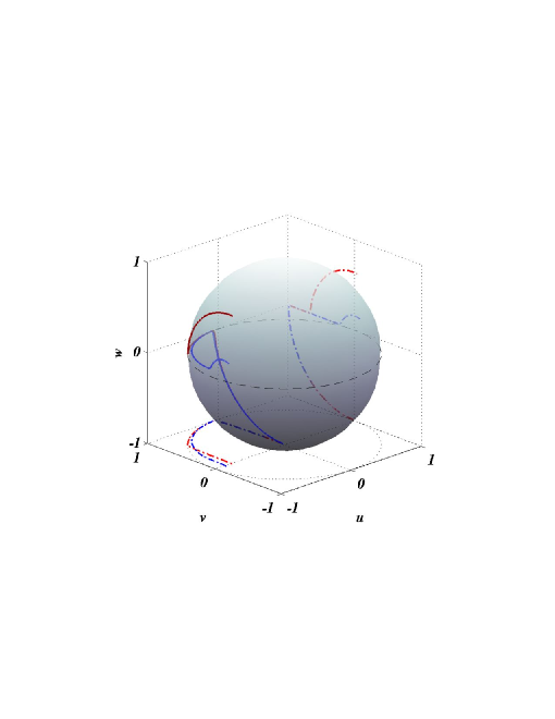
Figure 1: (color online) Collisional shift and loss of single-particle coherence in a Ramsey scheme. The solid red line traces the trajectory of the Bloch vector in the absence of interactions. When interactions are present (solid blue line), the frequency of phase oscillations is modified if $G_{gg}\neq G_{ee}$ and the length of the Bloch vector is not conserved when $G_{gg}+G_{ee}\neq 2G_{ge}$ (note that the solid blue curve deviates from the dashed great circle during the free induction decay, whereas the solid red curve does not).

The outline of the paper is a follows. In Sec. II we review the Ramsey separated oscillatory fields method for noninteracting particles and set up the notation we use in what follows. In Sec. III we construct a second-quantized model, describing the single-site Ramsey scheme for interacting bosons. This model is numerically solved in Sec. IV, demonstrating various collisional effects on Ramsey fringe patterns. Hopping between sites is introduced in Sec. V where we present two-site results and propose an inverted Rabi phase scheme to cancel collisional shifts. Conclusions are presented in Sec. VI.

II Ramsey separated oscillatory fields

Norman Ramsey introduced the method of separated oscillatory fields in 1950 Ramsey_50 . A long time-period between the application of two nearly resonant coherent fields makes the Ramsey resonance very narrow, and thus suitable for high-performance clocks and precision measurements Vanier_89 ; Lemonde_01 . The method has since become a widely used technique for determining resonance frequencies to high precision. For example, in the Cs fountain clock experiments summarized in Refs. Lemonde_01 ; Bauch_03 , the observed linewidth of the Ramsey resonance was 1 Hz, two orders of magnitude below that of thermal Cs clocks Bauch_03 ; Bauch_89 ; Bauch_02 .

For a two-level atom in an intense short near-resonant pulse with central frequency $\omega$, the Hamiltonian in the interaction representation with $|\psi\rangle=a_{g}(t)\exp(-i(\epsilon_{g}/\hbar+\omega)t)|g\rangle+a_{e}(t)\exp(-i\epsilon_{e}t/\hbar)|e\rangle$, and rotating wave approximation, takes the form

$$\mathbf{H}=\left(\begin{array}[]{cc}\Delta/2&\Omega^{*}/2\\ \Omega/2&-\Delta/2\end{array}\right)\,,$$ (1)

where $\Omega=2\mu A/\hbar$ is the Rabi frequency, $A$ is the slowly varying envelope of the electric field strength, $\mu$ is the transition dipole moment, and $\Delta=(\epsilon_{e}-\epsilon_{g}-\hbar\omega)/\hbar$ is the detuning from resonance of the laser frequency $\omega$. The solution of the optical Bloch equations for the two-level atom is given in terms of the unitary evolution operator for the two-level system for a real slowly varying envelope:

$$\mathbf{U}=\left(\begin{array}[]{cc}\cos(\frac{\Omega_{g}t}{2})-\frac{i\Delta}{\Omega_{g}}\sin(\frac{\Omega_{g}t}{2})&\frac{i\Omega}{\Omega_{g}}\sin(\frac{\Omega_{g}t}{2})\\ {}\hfil&{}\hfil\\ \frac{i\Omega}{\Omega_{g}}\sin(\frac{\Omega_{g}t}{2})&\cos(\frac{\Omega_{g}t}{2})+\frac{i\Delta}{\Omega_{g}}\sin(\frac{\Omega_{g}t}{2})\end{array}\right)\,.$$ (2)

Here $\Omega_{g}=\sqrt{|\Omega|^{2}+\Delta^{2}}$ is the generalized Rabi frequency. In the Ramsey method, the system, assumed to be initially in the ground state $|g\rangle$, is subjected to two pulses separated by a delay time $T$,

$$\Omega(t)=\left\{\begin{array}[]{ll}\Omega&\mbox{if $0\leq t\leq\tau_{p}$}\,,\\ 0&\mbox{if $\tau_{p}<t<T+\tau_{p}$}\,,\\ \Omega&\mbox{if $T+\tau_{p}\leq t\leq T+2\tau_{p}$}\,,\end{array}\right.$$ (3)

with $\Omega\tau_{p}=\pi/2$ and $T\gg\tau_{p}$. From transformation (2), it is clear that the effect of the first pulse is to evolve the initial ground state $|g\rangle$ into the state $(|g\rangle+i|e\rangle)/\sqrt{2}$. In a Bloch-sphere picture with $u=\Re(a_{g}^{*}a_{e})$, $v=\Im(a_{g}^{*}a_{e})$, and $w=(|a_{e}|^{2}-|a_{g}|^{2})/2$, the Bloch vector $(u,v,w)$ is projected by the first pulse into the $uv$ plane, as depicted by the red line in Fig. 1. During the delay time, the system carries out phase oscillations, corresponding to rotation of the Bloch vector in the $uv$ plane with frequency $\Delta$. Finally, the second pulse rotates the vector again by an angle of $\Omega_{g}\tau_{p}$ about the $u$ axis, as shown in Fig. 1. Fixing $\Delta$ and measuring the final projection of the Bloch vector on the $w$ axis as a function of $T$, one obtains fringes of fixed amplitude $\Omega/\Omega_{g}$ and frequency $\Delta$. Alternatively, fixing $T$ and measuring $w(t>T+2\tau_{p})$ as a function of the detuning $\Delta$, results in a power-broadened fringe pattern of amplitude $\Omega/\Omega_{g}$ and frequency $2\pi/T$. The resulting probability to be in the excited state is given by

$$P_{e}=\frac{4\Omega^{2}}{\Omega_{g}^{2}}\sin^{2}(\frac{1}{2}\Omega_{g}\tau_{p})\left(-\cos(\frac{1}{2}\Omega_{g}\tau_{p})\cos(\frac{1}{2}\Delta T)+\frac{\Delta}{\Omega_{g}}\sin(\frac{1}{2}\Omega_{g}\tau_{p})\sin(\frac{1}{2}\Delta T)\right)^{2}\,.$$ (4)

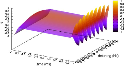
Figure 2: (color online) Population inversion $w$ versus time and detuning $\Delta$ in a Ramsey separated field method. The interaction strength is taken to be $\kappa=100$ Hz.

Figure 2 shows the population inversion $w$ versus time and detuning $\Delta$ using a Ramsey separated field method for one atom in an optical lattice site. The final time corresponds to the time at which the Ramsey clock signal is measured as a function of detuning $\Delta$, i.e., either the population of the ground or the excited state is measured as a function of $\Delta$. Note that the excited state population at the final time is unity at zero detuning and that the population inversion oscillates as a function of detuning.

It is easy to generalize this treatment to a time-dependent Rabi frequency $\Omega(t)=2\mu A(t)/\hbar$ due to a pulse of light which turns on and off with a finite rate in terms of the pulse area, $\int_{0}^{\tau_{p}}\Omega(t^{\prime})dt^{\prime}$. For a $\pi/2$ pulse, $\int_{0}^{\tau_{p}}\Omega(t^{\prime})dt^{\prime}=\pi/2$, where $\tau_{p}$ is the pulse duration. For the Ramsey pulses, $\int_{0}^{\tau_{p}}\Omega(t^{\prime})dt^{\prime}=\pi/2$, $\int_{\tau_{p}}^{T+\tau_{p}}\Omega(t^{\prime})dt^{\prime}=0$, and $\int_{T+\tau_{p}}^{T+2\tau_{p}}\Omega(t^{\prime})dt^{\prime}=\pi/2$.

III Second-quantized Ramsey model

In order to study the effects of collisions on Ramsey fringes obtained in a separated-fields scheme, we use a second-quantized formalism to treat a multiply-populated single site of the optical potential and calculate the Ramsey fringe dynamics. The many-body Hamiltonian for a system of two-level atoms, all in the same external motional state of a trap, can be written as Vardi01 ; Anglin_01

$$\hat{H}=\sum_{i=g,e}E_{i}\hat{a}^{\dagger}_{i}\hat{a}_{i}-\frac{\hbar\Omega(t)}{2}(\hat{a}^{\dagger}_{g}\hat{a}_{e}+\hat{a}^{\dagger}_{e}\hat{a}_{g})+\sum_{i,j=g,e}G_{ij}\hat{a}^{\dagger}_{i}\hat{a}^{\dagger}_{j}\hat{a}_{j}\hat{a}_{i}\,.$$ (5)

Here the subscripts $g$ and $e$ indicate the ground and excited states of the two level atom, and $\hat{a}_{i}$ is the annihilation operator for an atom in internal state $i$, where $i=g,e$. The self- and cross- atom-atom interaction strengths are denoted as $G_{ii}$ and $G_{ij}$ respectively, the internal energy of state $i$ is denoted as $E_{i}$, where $E_{g}=\epsilon_{g}+\hbar\omega$ and $E_{e}=\epsilon_{e}$. For bosonic atoms, the creation and annihilation operators satisfy the commutation relations

$$[\hat{a}_{i},\hat{a}_{j}^{\dagger}]=\delta_{ij}\,,\qquad[\hat{a}_{i}^{\dagger},\hat{a}_{j}^{\dagger}]=0\,,\qquad[\hat{a}_{i},\hat{a}_{j}]=0\,.$$ (6)

Defining the operators

$$\hat{n}_{i}=\hat{a}^{\dagger}_{i}\hat{a}_{i},\;\;\;\hat{N}=\hat{n}_{g}+\hat{n}_{e},\;\;\;\hat{L}_{z}={\hat{n}_{g}-\hat{n}_{e}\over 2},\;\;\;\hat{L}_{x}={\hat{a}^{\dagger}_{g}\hat{a}_{e}+\hat{a}^{\dagger}_{e}\hat{a}_{g}\over 2},\;\;\;\hat{L}_{y}={\hat{a}^{\dagger}_{g}\hat{a}_{e}-\hat{a}^{\dagger}_{e}\hat{a}_{g}\over 2i},$$ (7)

the Hamiltonian can be written as

$$\hat{H}=E\hat{N}+\hbar\Delta\hat{L}_{z}-\hbar\Omega(t)\hat{L}_{x}+\sum_{i=1}^{2}G_{ii}(\hat{n}_{i}^{2}-\hat{n}_{i})+2G_{ge}\hat{n}_{g}\hat{n}_{e}\,,$$ (8)

where

$$E = (\hbar\omega+\epsilon_{g}+\epsilon_{e})/2\,,$$ (9)

$$\hbar\Delta = (\hbar\omega-\epsilon_{e}+\epsilon_{g})\,.$$ (10)

Since $\hat{N}$ commutes with $\hat{H}$, the Hamiltonian conserves the total number of particles. Typically, in a Ramsey-fringe experiment, the initial state is assumed to have all $N$ atoms in the ground state $|g\rangle$. Fixing $\hat{N}=N$ in the single site that we are considering here (i.e., so that there are no fluctuations), and using the identities $\hat{n}_{g}=\hat{N}/2+\hat{L}_{z}$ and $\hat{n}_{e}=\hat{N}/2-\hat{L}_{z}$, we finally obtain

$$\hat{H} = (E-{G_{gg}+G_{ee}\over 2})\hat{N}+(G_{gg}+G_{ee}+2G_{ge}){\hat{N}^{2}\over 4}$$ (11)

$$-\hbar\Omega(t)\hat{L}_{x}+[\hbar\Delta+(G_{gg}-G_{ee})(\hat{N}-1)]\hat{L}_{z}$$

$$+(G_{gg}+G_{ee}-2G_{ge})\hat{L}_{z}^{2}\,.$$

Since Ramsey spectroscopy measures essentially single-particle coherence, we will be interested in the dynamics of the reduced single-particle density matrix (SPDM) $\rho(t)$:

$$\rho(t)=\langle\hat{\rho}(t)\rangle=\frac{N}{2}{\mathcal{I}}+u(t)\sigma_{x}+v(t)\sigma_{y}+w(t)\sigma_{z}\,,$$ (12)

where $\hat{\rho}(t)=\hat{a}_{i}^{\dagger}(t)\hat{a}_{j}(t)$ is the reduced single-particle density operator, ${\mathcal{I}}$ is a two-by-two unity matrix, $\sigma_{i},i=x,y,z$ are Pauli matrices, and $u=\langle\hat{L}_{x}\rangle$, $v=\langle\hat{L}_{y}\rangle$, $w=\langle\hat{L}_{z}\rangle$ are the components of the single-particle Bloch vector, corresponding to the real- and imaginary parts of the single-particle coherence, and to the population imbalance between the two modes, respectively. The expectation values, $\langle\cdot\rangle$ are over the $N$-particle states. The Liouville-von-Neuman equation for the SPDM,

$${d\over dt}\rho={i\over\hbar}\langle[\hat{\rho},\hat{H}]\rangle={i\over\hbar}\sum_{j=x,y,z}\langle[\hat{L}_{j},\hat{H}]\rangle\,\sigma_{j}~{},$$ (13)

is thus equivalent to the expectation values of the three coupled Heisenberg equations of motion for the $SU(2)$ generators,

$${d\over dt}\hat{L}_{x} = -[\Delta+{\mathcal{U}}(\hat{N}-1)]\hat{L}_{y}-{\mathcal{G}}(\hat{L}_{y}\hat{L}_{z}+\hat{L}_{z}\hat{L}_{y}),$$ (14)

$${d\over dt}\hat{L}_{y} = [\Delta+{\mathcal{U}}(\hat{N}-1)]\hat{L}_{x}+{\mathcal{G}}(\hat{L}_{x}\hat{L}_{z}+\hat{L}_{z}\hat{L}_{x})$$ (15)

$$+\Omega(t)\hat{L}_{z}~{},$$

$${d\over dt}\hat{L}_{z} = -\Omega(t)\hat{L}_{y}\,,$$ (16)

where we denote the linear and nonlinear interaction strength parameters respectively by

$${\mathcal{U}}\equiv(G_{gg}-G_{ee})/\hbar~{},$$ (17)

$${\mathcal{G}}\equiv(G_{gg}+G_{ee}-2G_{ge})/\hbar~{}.$$ (18)

In order to study effects resulting in from the coupling to an environment consisting of a bath of external degrees of freedom, we use the master equation Carmichael_93 ; Gardiner_99

$${d\over dt}\hat{\rho}={i\over\hbar}[\hat{\rho},\hat{H}]-\sum_{k}\Gamma_{k}(2\hat{O}_{k}\hat{\rho}\hat{O}_{k}^{{\dagger}}-\{\hat{O}_{k}^{{\dagger}}\hat{O}_{k},\hat{\rho}\})\,,$$ (19)

where the second term on the right hand side of (19) has the Markovian Lindblad form Lindblad and gives rise to dissipation effects of the bath on the density operator. Such terms may be used to depict decay due to spontaneous emission, atom-surface interactions, motional effects, black-body radiation and other environmental effects. The Lindblad operators $\hat{O}_{k}$ are determined from the nature of the system-bath coupling and the coefficients $\Gamma_{k}$ are the corresponding coupling parameters. In what follows we shall assume that the most significant dissipation process is dephasing, and we neglect all other dissipation effects (e.g., we assume spontaneous emission is negligible because the lifetime of the excited state is much longer than the Ramsey process run-time, etc.). Thus, the Lindblad operator is taken to be ${\hat{L}}_{z}$, yielding dephasing of the transition dipole moment without affecting the population of the ground or excited states. We shall only study this type of $t_{2}$ dephasing, without fully exploring the effects of other types of Lindblad operators. Clearly, it is easy to generalize this and consider the effects of additional Lindblad operators, but we do not do so here. Moreover, non-Markov treatments can be used to generalize the Markovian approximation made in deriving Eq. (19) Carmichael_93 ; Gardiner_99 .

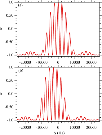
Figure 3: (color online) Linear collisional shift. Ramsey fringes for $N$ particles in a lattice site, for (a) ${\mathcal{U}}={\mathcal{G}}=0$ and (b) ${\mathcal{U}}(N-1)=3000$ Hz, ${\mathcal{G}}=0$.

IV Single-site many-body dynamics

We first study how interparticle interactions can modify the Bloch-vector dynamics in a single-site Ramsey scheme. From Eq. (11) and Eqs. (14)-(16) it is evident that there are three possible collisional effects. First, differences between the interaction strengths of ground and excited atoms, will induce a linear frequency shift of the center of the Ramsey fringe pattern by an amount ${\mathcal{U}}(N-1)$. This effect is illustrated in Fig. 1, where the trajectory of the Bloch vector during a Ramsey sequence is traced in the absence of interactions (red) and in their presence (blue). Clearly, the frequency of oscillation in the $uv$ plane during the delay time $T$ is modified by the interaction. In Fig. 3 we plot the resulting fringe pattern when ${\mathcal{G}}$ is set equal to zero. Fig. 3(a) depicts the Ramsey fringes without any interaction, ${\mathcal{U}}={\mathcal{G}}=0$, whereas in Fig. 3(b) we plot the fringe pattern with ${\mathcal{U}}=3000$ Hz. Since for ${\mathcal{G}}=0$ Eqs. (14)-(16) remain linear, and the only effect is a linear frequency shift. The whole curve $w(\Delta)$ versus $\Delta$ is simply shifted in $\Delta$ by an amount ${\mathcal{U}}(N-1)$.

Also shown in Fig. 1 is the loss of single-particle coherence due to interparticle entanglement Vardi01 . This dephasing process is only possible for the nonlinear case when ${\mathcal{G}}\neq 0$. It is manifested in the reduction of the single-particle purity $p=\mathrm{Tr}(\rho^{2})=|u|^{2}+|v|^{2}+|w|^{2}$, during the evolution. In comparison, for the single-particle case depicted in red, single-particle purity is trivially conserved and the length of the Bloch vector is unity throughout the propagation time; the Bloch vector at the end of the process sits well within the Bloch sphere.

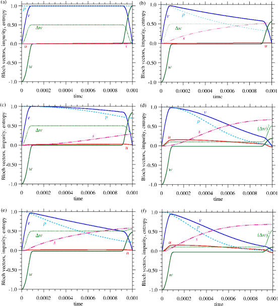
Figure 4: (color online) Bloch vector, $u$, $v$, $w$, purity $p$, entropy $s$ and variance of $w$ versus time using a Ramsey separated field method for zero detuning $\Delta$. (a) Two atoms without dephasing and without interaction. (b) Two atoms with dephasing ($\Gamma_{L_{z}}=100$ Hz) and without interaction. (c) Two atoms without dephasing but with interaction ($\kappa=100$ Hz). (d) Ten atoms without dephasing but with interaction ($\kappa=100$ Hz). (e) Two atoms with dephasing ($\Gamma_{L_{z}}=100$ Hz) and interaction ($\kappa=100$ Hz). (e) Ten atoms with dephasing and interaction.

The decay of single particle coherence due to entanglement is illustrated in Fig. 4, where the Bloch vector ($u$, $v$, $w$,), the single particle purity $p$, the single-particle entropy $s=\mathrm{Tr}(\rho\ln\rho)=-\,\ln[(1+\sqrt{p})^{1+\sqrt{p}}(1-\sqrt{p})^{1-\sqrt{p}}/4]/2$, and the variance of $w$, $\Delta w$, are plotted versus time in a Ramsey separated field method for $\Delta=0$. The total time for the Ramsey process is taken to be $t_{\mathrm{tot}}=T+2\tau_{p}=1.0\times 10^{-3}$ s, with the first and second Ramsey pulses each of duration $t_{\mathrm{tot}}/12$, and the Rabi frequency of the pulses are $3.0\times 10^{3}$ Hz, so the two pulses each have pulse area $\pi/2$. The interaction strengths were arbitrarily set to $G_{ee}=G_{ge}=0$, so that ${\mathcal{U}}={\mathcal{G}}=G_{gg}/\hbar\equiv\kappa$. In frame (a) $\kappa$ is set to zero (corresponding to the case of one atom per site in the optical lattice). The effect of decoherence due to the $\Gamma_{L_{z}}$ term in Eq. (13) is shown in frame (b), while collisional dephasing is depicted in frames (c)-(e) were we set $\kappa=100$ Hz. In frames (c) and (e) we have taken two atoms per site, whereas in frames (d) and (f) we have taken 10 atoms per site. In frames (e) and (f), dephasing with strength $\gamma_{z}=1.0\times 10^{2}$ Hz is included. From comparison of Fig. 4(b) and Fig. 4(c-d), it is clear that the loss of single-particle coherence due to entanglement is similar to the effect of dephasing due to coupling to an external bath. In particular, the final population inversion is strongly affected. Comparing Figs. 4(b) and Fig. 4(c), it is clear that collisional dephasing is stronger as the number of particles grows. The combined effect of decoherence and interparticle entanglement is shown in frames (e) and (f).

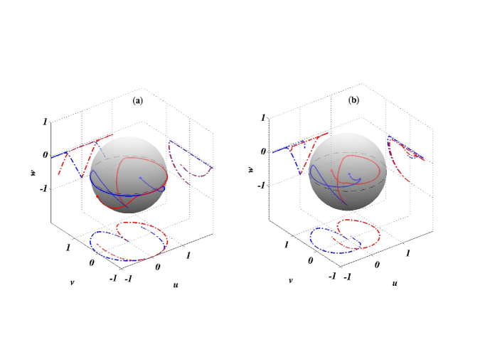
Figure 5: (color online) Collisional asymmetry of Ramsey fringes. Red and blue curves correspond to Bloch-vector trajectories with positive and negative detuning, respectively. The final position of the Bloch vectors is indicated by a dot at the end of the trajectories. In the absence of interactions (a) the final projection onto the $w$ axis is independent of the sign of $\Delta$. However, when interactions are present (b) nonlinear collisional shifts break the symmetry. Dash-dotted lines depict projections of the trajectory onto the $uv$, $uw$, and $vw$ planes.

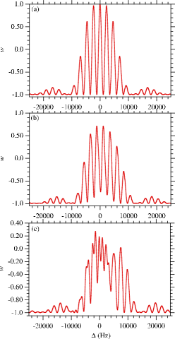
Figure 6: (color online) Asymmetric Ramsey fringes. Numerically calculated Ramsey fringe patterns, at three different values of the nonlinear interaction: (a) ${\mathcal{G}}=0$, ${\mathcal{U}}=0$, (b) ${\mathcal{G}}=1500Hz$, ${\mathcal{U}}=0$, and (c) ${\mathcal{G}}=3000$ Hz, ${\mathcal{U}}=0$.

Yet another collisional effect is caused by the ${\mathcal{G}}\hat{L}_{z}^{2}$ term in the Hamiltonian (11). In the mean-field approximation, replacing $\hat{L}_{i}$ by their expectation values, this term leads to a nonlinear frequency shift of $2{\mathcal{G}}w(\tau_{p})$, where $w(\tau_{p})$ is the value of the population imbalance after the first pulse. As illustrated in Figs. 5 and 6, the nonlinear shift results in an asymmetric fringe pattern, because for ${\mathcal{G}}\neq 0$, $w(\tau_{p})$ depends on the sign of $\Delta$ during the first pulse. Without interactions, when ${\mathcal{U}}={\mathcal{G}}=0$, the dynamical equations (14)-(16) are symmetric under $\Delta\rightarrow-\Delta~{},~{}\hat{L}_{x}\rightarrow-\hat{L}_{x}$. This symmetry shows up in Fig. 5(a) where the evolution with two opposite values of $\Delta$ is traced over the Bloch sphere. As shown in the various projections onto the $uv$, $vw$, and $uw$ planes, $u_{\Delta}(t)=-u_{-\Delta}(t)$, $v_{\Delta}(t)=v_{-\Delta}(t)$, and $w_{\Delta}(t)=w_{-\Delta}(t)$, where $(u_{\Delta}(t),v_{\Delta}(t),w_{\Delta}(t))$ denote the Bloch vector $(u(t),v(t),w(t))$, evolved in a Ramsey sequence with detuning $\Delta$. Similarly, when ${\mathcal{G}}=0$ and ${\mathcal{U}}$ is nonvanishing, the resulting shifted pattern is still symmetric about $\Delta=-(N-1){\mathcal{U}}$ since the dynamical equations are invariant under $\Delta+(N-1){\mathcal{U}}\rightarrow-(\Delta+(N-1){\mathcal{U}})~{},~{}\hat{L}_{x}\rightarrow-\hat{L}_{x}$. However, for finite values of ${\mathcal{G}}$ the symmetry breaks down because the last terms on the r.h.s. of Eqs. (14) and (15) change sign, as demonstrated in Fig. 5(b). Consequently, when the final projection on the $w$ axis is plotted as a function of the detuning $\Delta$, we obtain asymmetric fringe patterns. In Fig. 6, we compare the symmetric single-particle pattern (Fig. 6a) with asymmetric two-particle Ramsey fringes obtained with nonvanishing values of ${\mathcal{G}}$ (Figs. 6b and 6c). The linear shift ${\mathcal{U}}$ is set equal to zero for all plots. Both the asymmetry of the emerging lineshape and the reduction in fringe contrast due to collisional dephasing are evident.

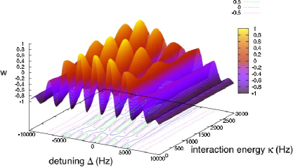
Figure 7: (color online) Population inversion $w$, versus detuning $\Delta$ and interaction strength ${\mathcal{U}}={\mathcal{G}}=\kappa$ in a Ramsey separated field configuration at the final time after the second pulse.

The combined effect of the linear shift and the nonlinear term in Eqs. (14)-(16) is shown in Fig. 7 where the final population inversion $w(t=\tau+2\tau_{p})$ is plotted as a function of the detuning $\Delta$ and the interaction strength, set arbitrarily to ${\mathcal{U}}={\mathcal{G}}=\kappa$. Fringe maxima are located about $(\Delta+\kappa(N-1)+2\kappa w(\tau_{p}))=2j\pi$ where $j$ is an integer and $w(\tau_{p})$ depends on both $\Delta$ and $\kappa$. As $\kappa$ increases, collisions shift the peak intensity and the fringe contrast is reduced due to collisional dephasing.

V Two-site Many-Body Dynamics

Having established how interparticle interactions affect the Ramsey lineshapes in a multiply-occupied single lattice site, we proceed to consider an optical lattice with multiple sites labeled by the site index $\alpha$. Each site is populated with atoms that can be in any one of two levels, the ground state level $|g\rangle$ and the excited state level $|e\rangle$, coupled through a Rabi flopping term in the Hamiltonian. The full Hamiltonian is given by

$$\hat{H} = \sum_{\langle\alpha,\beta\rangle}\hat{H}_{\mathrm{hop}}^{(\alpha,\beta)}$$

$$+\sum_{\alpha}\left[\hat{H}_{\mathrm{int}}^{(\alpha)}+\hat{H}_{\mathrm{diff}}^{(\alpha)}+\hat{H}_{\mathrm{sum}}^{(\alpha)}+\hat{H}_{\mathrm{R}}^{(\alpha)}\right]\ ,$$

$$\hat{H}_{\mathrm{hop}}^{(\alpha,\beta)} = \hbar J_{\mathrm{hop}}[(\hat{a}^{\dagger}_{\alpha}\hat{a}_{\beta}+h.c.)+(\hat{b}^{\dagger}_{\alpha}\hat{b}_{\beta}+h.c.)]\ ,$$ (20b)

$$\hat{H}_{\mathrm{int}}^{(\alpha)} = \tfrac{1}{2}U_{aa}\hat{a}^{\dagger}_{\alpha}\hat{a}^{\dagger}_{\alpha}\hat{a}_{\alpha}\hat{a}_{\alpha}+\tfrac{1}{2}U_{bb}\hat{b}^{\dagger}_{\alpha}\hat{b}^{\dagger}_{\alpha}\hat{b}_{\alpha}\hat{b}_{\alpha}$$ (20c)

$$+U_{ab}\hat{a}^{\dagger}_{\alpha}\hat{b}^{\dagger}_{\alpha}\hat{b}_{\alpha}\hat{a}_{\alpha}\ ,$$

$$\hat{H}_{\mathrm{diff}}^{(\alpha)} = \frac{\hbar\Delta}{2}(\hat{a}^{\dagger}_{\alpha}\hat{a}_{\alpha}-\hat{b}^{\dagger}_{\alpha}\hat{b}_{\alpha})\ ,$$ (20d)

$$\hat{H}_{\mathrm{sum}}^{(\alpha)} = \frac{\epsilon_{a}+\hbar\omega+\epsilon_{b}}{2}(\hat{a}^{\dagger}_{\alpha}\hat{a}_{\alpha}+\hat{b}^{\dagger}_{\alpha}\hat{b}_{\alpha})\ ,$$ (20e)

$$\hat{H}_{\mathrm{R}}^{(\alpha)} = \frac{\hbar\Omega(t)}{2}(\hat{a}^{\dagger}_{\alpha}\hat{b}_{\alpha}e^{i\phi_{\alpha}(t)}+\hat{b}^{\dagger}_{\alpha}\hat{a}_{\alpha}e^{-i\phi_{\alpha}(t)})\ .$$ (20f)

Here, the operators $a$ and $b$ are bosonic destruction operators for atoms in the two states $|g\rangle$ and $|e\rangle$, and the indices $\alpha$ and $\beta$ run over the lattice sites, with $\langle\alpha,\beta\rangle$ denoting a pair of adjacent sites. The constants $J_{\mathrm{hop}}$ and $U_{ij}$, $i,j=g,e$, are the strength of the hopping to neighboring sites in $H_{\mathrm{hop}}$ and the effective on-site interaction in $H_{\mathrm{int}}$, respectively. $H_{\mathrm{diff}}$ and $H_{\mathrm{sum}}$ are the energy difference and average of the dressed states of the atoms, and $H_{R}$ induces Rabi transitions between the two atomic internal states with Rabi frequency $\Omega(t)$ and phase $\phi_{\alpha}(t)$, which are related to the intensity and phase of the laser which induces these transitions. The Hamiltonian in (20) is identical to what we used in previous sections, except for the addition of the hopping term $\hat{H}_{\mathrm{hop}}$ that can result in hopping of particles to adjacent sites with rate $J_{\mathrm{hop}}$.

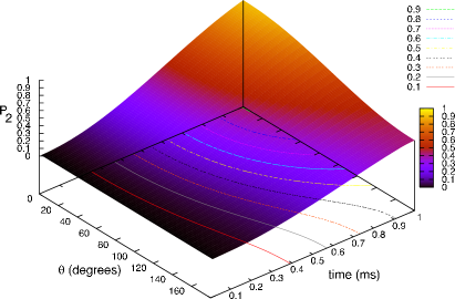
Figure 8: (color online) Probability for double occupancy $P_{2}$, during a Ramsey sequence with $\Delta=0$, versus relative Rabi-drive phase angle $\theta$ for $J_{\mathrm{hop}}=100$ Hz. Tunneling is suppressed for $\theta=\pi$ due to destructive interference and enhanced for $\theta=0$ due to constructive interference. Interparticle interactions are set equal to zero.

Note that the phase $\phi_{\alpha}(t)$ can depend upon the site index $\alpha$. Consider, for simplicity, a 1D optical lattice along the $x$ axis, and a plane wave field with detuning $\Delta$ from resonance with wave vector ${\mathbf{k}}$. The Rabi frequency at site $\alpha$ is given by $\Omega({\mathbf{r}}_{\alpha},t)=\Omega(t)\exp[i{\mathbf{k}}\cdot{\mathbf{r}}_{\alpha}]=\Omega(t)\exp(ik_{x}x_{\alpha})$. Thus, there is a phase difference $\theta$ between the Rabi frequency at neighboring sites, $\theta=k_{x}\delta x$, where $\delta x$ is the lattice spacing. The angle between the wave vector ${\mathbf{k}}$ and the $x$ axis can be adjusted to control the phase difference $\theta=\phi_{\alpha}-\phi_{\alpha-1}$. In what follows, we show that a proper choice of the relative phase angle $\theta$ between Rabi drive fields in adjacent sites may be used to suppress the tunneling between them and thus reduce collisional shifts. When $J_{\mathrm{hop}}=0$, there is no relevance to the phases $\phi_{\alpha}(t)$ (they do not affect the dyanmics), but as soon as hopping from one site to an adjacent site is allowed, these phases can affect the dynamics.

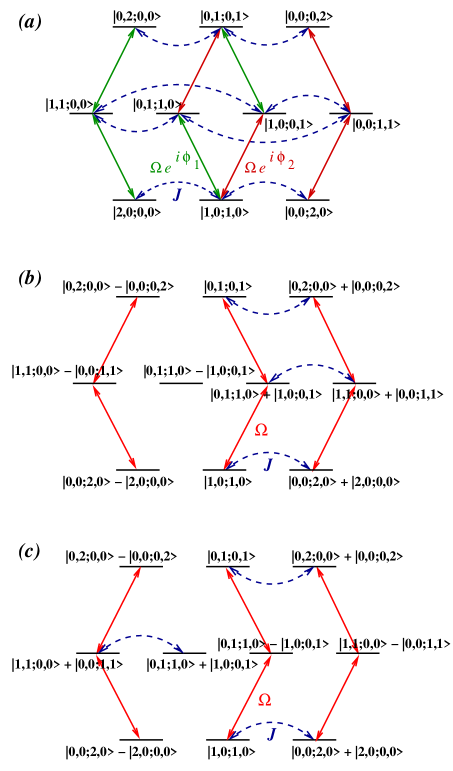
Figure 9: (color online) Two-particle level schemes for Ramsey spectroscopy in the presence of tunneling: (a) general scheme (b) coupling between parity eigenstates for $\theta=0$ (c) coupling between parity eigenstates for $\theta=\pi$. Rabi coupling between ground- and excited states, is denoted by red and green solid arrows, corresponding to different phases of the driving fields in adjacent sites. Blue dashed arrows denote hopping between sites. Fock states are denoted as $|n^{g}_{1},n^{e}_{1};n^{g}_{2},n^{e}_{2}\rangle$, wh ere $n^{g}_{\alpha}=\langle\hat{a}_{\alpha}^{\dagger}\hat{a}_{\alpha}\rangle$ and $n^{e}_{\alpha}=\langle\hat{b}_{\alpha}^{\dagger}\hat{b}_{\alpha}\rangle$.

We expect that for sufficiently low densities, the probability of finding more than two adjacent populated sites is very small. It is therefore possible to capture much of the physics of the hopping process, using a two-site model. At higher densities, more elaborate models should be used. In Fig. 8 we plot numerical results for two particles in two sites ($N=2,\alpha=1,2$) for $J_{\mathrm{hop}}=100$ Hz, showing the probability of double occupancy during a Ramsey fringe sequence in the presence of tunneling, as a function of the relative angle $\theta$. The parameters used are the same as those used previously, except that now we allow for hopping, and therefore $J_{\mathrm{hop}}$ and the angle $\theta$ affects the dynamics. The initial conditions correspond to a single atom in its ground state in each lattice site before the Ramsey process begins. When both atoms are driven in-phase ($\theta=0$), tunneling takes place, leading to multiple occupancy. The tunneling is significantly suppressed for a $\theta=\pi$ phase difference between the Rabi drives in adjacent sites. As shown in Fig. 9, this suppression originates from destructive interference. In Fig. 9a we plot the level scheme for a two-particle, two-site system. The levels $|n^{g}_{1},n^{e}_{1};n^{g}_{2},n^{e}_{2}\rangle$ denote Fock states with $n^{g}_{\alpha}$ and $n^{e}_{\alpha}$ particles in the ground- and excited states respectively, of site $\alpha$. Depending on the relative phase between the optical drive fields, tunneling from states with a ground state atom in one site and an excited atom in another, can interfere constructively or destructively. Therefore, as seen in Fig. 9b and Fig. 9c, tunneling can only take place between even-parity states. For in-phase Rabi drive $\theta=0$ (Fig. 9b), the initial even-parity state $|1,0;1,0\rangle$ is coupled by a single optical excitation to the even-parity state $(1/\sqrt{2})\left(|0,1;1,0\rangle+|1,0;0,1\rangle\right)$, for which the two tunneling pathways interfere constructively. In contrast, for out-of-phase drive $\theta=\pi$ (Fig. 9c), the first $\pi/2$ pulse drives the system partially into the odd-parity state $(1/\sqrt{2})\left(|0,1;1,0\rangle-|1,0;0,1\rangle\right)$ which is ’dark’ to tunneling, leading to a reduced probability of multiple occupancy during the time evolution.

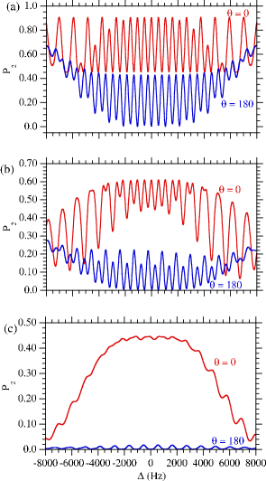
Figure 10: (color online) Probability of double-occupation at the end of a Ramsey sequence versus detuning, for different values of the nonlinearity ${\mathcal{U}}={\mathcal{G}}=\kappa$: (a) $\kappa=0$, (b) $\kappa=5.0\times 10^{2}$, and (c) $\kappa=1.0\times 10^{3}$. Red curves correspond to $\theta=0$ whereas blue curves show the lineshape for $\theta=\pi$.

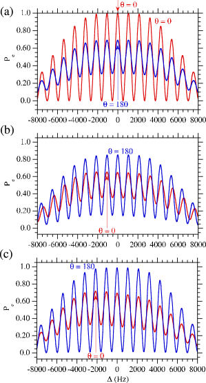
Figure 11: (color online) Ramsey fringe patterns for different values of the nonlinearity ${\mathcal{U}}={\mathcal{G}}=\kappa$: (a)$\kappa=0$, (b) $\kappa=5.0\times 10^{2}$, and (c) $\kappa=1.0\times 10^{3}$. Red curves correspond to $\theta=0$ whereas blue curves show the lineshape for $\theta=\pi$. The arrows serve to roughly indicate the centers of the distributions.

The lower probability of finding multiply occupied sites in an inverted-phase Rabi-drive configuration, is manifested in the emerging Ramsey fringe patterns. In Fig. 10 we plot the probability of double-occupancy at the end of a Ramsey sequence, as a function of detuning, for different degrees of nonlinearity which is arbitrarily set to ${\mathcal{U}}={\mathcal{G}}=\kappa$. While increasing nonlinearity generally tends to localize population and reduce tunneling, the probability of finding both particles in the same lattice site is always lower for out-of-phase driving. The resulting Ramsey lineshapes are plotted in Fig. 11, clearly demonstrating reduced collisional effects for $\theta=\pi$ (blue curves), compared to the in-phase driving fields scheme (red curves). The center of the distributions for $\theta=0$ are clearly strongly shifted from $\Delta=0$, and much less shifted for $\theta=\pi$. This reduced shift in the center of the distribution is, of course, of central importance for a clock.

VI Conclusion

Optical lattice atom clocks hold great promise for setting frequency standards. In order to achieve high accuracy with boson atoms, collisional frequency shifts have to be taken in account. We have shown that collisions can degrade Ramsey lineshapes by shifting their centers, rendering them asymmetric, and by reducing fringe-visibility due to the loss of single-particle coherence. Considering two adjacent populated sites in a 1D optical lattice configuration, we propose a method of reducing dynamical multiple population of lattice sites, based on driving different sites with different phases of the Rabi drive. Due to destructive interference between tunneling pathways leading to states with one ground and one excited atom in the same site, hopping is reduced and collisional effects are canceled out. It is difficult to see how to implement this kind of interference in a 2D or 3D configuration.

While collisional effects are considered here as an unwanted degrading factor, our work also suggests the potential application of the Ramsey separated field method for studying entanglement.

- (1) A. Bauch and H. R. Telle, Rep. Prog. Phys. 65, 789-843 (2002); J. Levine, Rev. Sci. Inst. 70, 2568 (1999); Y. Sortais et al., Physica Scripta T95, 50-57 (2001); P. Lemonde et al., Frequency Measurement and Control advanced techniques and future trends 79, 131 (2000); R. S. Conroy, Contemporary Physics 44, 99 (2003); M. D. Plimmer, Physica Scripta 70, C10 (2004); S. A. Diddams, J. C. Bergquist, S. R. Jefferts, and C. W. Oates, Science 306, 1318 (2004).
- (2) H. Katori and M. Takamoto, Phys. Rev. Lett. 91, 173005 (2003).
- (3) M. Takamoto, and H. Katori, Phys. Rev. Lett. 91, 223001 (2003); M. Takamoto, F.-L. Hong, R. Higashi, and H. Katori, Nature 435, 321 (2005).
- (4) R. Santra, E. Arimondo, T. Ido, C. H. Greene, and J. Ye, Phys. Rev. Lett. 94 (2005). See also, T. Hong, C. Cramer, W. Nagourney, and E. N. Fortson, Phys. Rev. Lett. 94, 050801 (2005).
- (5) D. E. Chang, J. Ye and M. D. Lukin, Phys. Rev. A69, 023810 (2004); A. D. Ludlow, M. M. Boyd, T. Zelevinsky, S. M. Foreman, S. Blatt, M. Notcutt, T. Ido, and J. Ye, Phys. Rev. Lett. 96, 033003 (2006); Z. W. Barber, C. W. Hoyt, C. W. Oates, L. Hollberg, A. V. Taichenachev, and V. I. Yudin, Phys. Rev. Lett. 96, 083002 (2006); A. Brusch, R. Le Targat, X. Baillard, M. Fouché, and Pierre Lemonde, Phys. Rev. Lett. 96, 103003 (2006).
- (6) A. V. Taichenachev, V. I. Yudin, C. W. Oates, C. W. Hoyt, Z. W. Barber, and L. Hollberg, Phys. Rev. Lett. 96, 083001 (2006).
- (7) Z. W. Barber, C. W. Hoyt, C. W. Oates, L. Hollberg, A. V. Taichenachev, and V. I. Yudin, Phys. Rev. Lett. 96, 083002 (2006).
- (8) R. H. Dicke, Phys. Rev. 89, 472 (1953); P. Lemonde and P. Wolf, Phys. Rev. A72, 033409 (2005).
- (9) Th. Udem, J. Reichert, R. Holzwarth, and T. W. Hänsch, Phys. Rev. Lett. 82, 3568?-3571 (1999); D. J. Jones, et al., Science 288, 635 (2000).
- (10) For a discussion of loading an optical lattice from a BEC, see P. S. Julienne, C. J. Williams, Y. B. Band, and M. Trippenbach, Phys. Rev. A72, 053615 (2005). We are not aware of a similar study for loading fermionic atoms into an optical lattice.
- (11) N. Ramsey, Phys. Rev. 78, 695 (1950); N. Ramsey, Molecular Beams (Oxford Univ. Press, Oxford 1985).
- (12) J. Vanier and C. Audoin, The Quantum Physics of Atomic Frequency Standards, (Adam Hilger IOP Publishing Ltd., Bristol, 1989), Chapter 5.
- (13) P. Lemonde, et al., “Cold-Atom Clocks on Earth and in Space”, in Frequency Measurement and Control, (Springer-Verlag, Berlin, 2001); Topics Appl. Phys. 79, 131-153 (2001).
- (14) A. Bauch, Meas. Sci. Technol. 14, 1159 (2003).
- (15) A. Bauch and T. Heindorff, “The primary cesium atomic clocks of the PTB”, In Proc. Fourth Symposium on Frequency Standards and Metrology, A. DeMarchi (Ed.), (Springer, Berlin, Heidelberg 1989) pp. 370-373.
- (16) A. Bauch and H. R. Telle, Reports Prog. Phys. 65, 798 (2002).
- (17) G. Lindblad, Commun. Math. Phys. 48, 119 (1976).
- (18) H. Carmichael, An Open System Approach to Quantum Optics, Springer Lecture Notes in Physics, (Berlin, Heidelberg, 1993).
- (19) C. W. Gardiner, P. Zoller, Quantum Noise: A Handbook of Markovian and Non-Markovian Quantum Stochastic Methods With Applications to Quantum Optics, (Springer, Berlin, 1999).
- (20) A. Vardi and J. R. Anglin, Phys. Rev. Lett. 86, 568 (2001).
- (21) J. R. Anglin and A. Vardi, Phys. Rev. A64, 13605 (2001).
- (22) M. Olshanii, Phys. Rev. Lett. 81, 938 (1998).
- (23) Y. B. Band and M. Trippenbach, Phys. Rev. A65, 053602 (2002).
- (24) W.M. Itano, J.C. Bergquist, J.J. Bollinger, I.M. Gilligan, D.J. Heinzen, F.L. Moore, M.G. Raizen, and D.J. Wineland, Phys. Rev. A. 47, 3554 (1993).
- (25) D.J. Wineland, J.J. Bollinger, W.M. Itano, J.C. Bergquist, and D.J. Heinzen, Phys. Rev. A. 50, 67 (1994).