All-optical switching, bistability, and slow-light transmission
in photonic crystal waveguide-resonator structures

Abstract

We analyze the resonant linear and nonlinear transmission through a photonic crystal waveguide side-coupled to a Kerr-nonlinear photonic crystal resonator. Firstly, we extend the standard coupled-mode theory analysis to photonic crystal structures and obtain explicit analytical expressions for the bistability thresholds and transmission coefficients which provide the basis for a detailed understanding of the possibilities associated with these structures. Next, we discuss limitations of standard coupled-mode theory and present an alternative analytical approach based on the effective discrete equations derived using a Green’s function method. We find that the discrete nature of the photonic crystal waveguides allows a novel, geometry-driven enhancement of nonlinear effects by shifting the resonator location relative to the waveguide, thus providing an additional control of resonant waveguide transmission and Fano resonances. We further demonstrate that this enhancement may result in the lowering of the bistability threshold and switching power of nonlinear devices by several orders of magnitude. Finally, we show that employing such enhancements is of paramount importance for the design of all-optical devices based on slow-light photonic crystal waveguides.

I Introduction

It is believed that future integrated photonic circuits for ultrafast all-optical signal processing require different types of nonlinear functional elements such as switches, memory and logic devices. Therefore, both novel physics and novel designs of such all-optical devices have attracted significant research efforts during the last two decades, and most of these studies utilize the concepts of optical switching and bistability Gibbs:1985:Book .

One of the simplest bistable optical devices which can find applications in photonic integrated circuits is a two-port device which is connected to other parts of a circuit by one input and one output waveguide. Its transmission properties depend on the intensity of light sent to the input waveguide. Two basic realizations of such a device can be provided by either direct or side-coupling between the input and output waveguides to an optical resonator. In the first case, we obtain a system with resonant transmission in a narrow frequency range, while in the second case, we obtain a system with resonant reflection. Both systems may exhibit optical bistability when the resonator is made of a Kerr nonlinear material. The resonant two-port systems of the first type, with direct-coupled resonator, can be realized in one-dimensional systems, and they have been studied in great details in the context of different applications. In contrast, the resonant systems of the second type, with side-coupled resonators, can only be realized in higher-dimensional structures, and their functionalities are not yet completely understood.

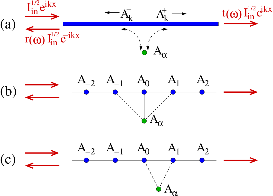
Figure 1: (Color online) Three types of the geometries of a straight photonic-crystal waveguide side-coupled to a nonlinear optical resonator, $A_{\alpha}$. Standard coupled-mode theory is based on the geometry (a) which does not account for discreteness-induced effects in the photonic-crystal waveguides. For instance, light transmission and bistability are qualitatively different for (b) on-site and (c) inter-site locations of the resonator along waveguide and this cannot be distinguished within the conceptual framework of structure of type (a).

Our goal in this paper is to study in detail the second class of resonant systems based on straight optical waveguides side-coupled to resonators as shown in Fig. 1. Moreover, we assume that the waveguide and resonator are created in two- or three-dimensional photonic crystal (PhC) PhCs . Due to a periodic modulation of the refractive index of PhCs, such structures may possess complete photonic band gaps, i.e. regions of optical frequencies where PhCs act as ideal optical insulators. Embedding carefully designed cavities into PhCs, one can create ultra-compact photonic crystal devices which are very promising for applications in photonic integrated circuits. As an illustration, side-coupled waveguide-resonator systems created in PhCs through arrays of cavities are schematically depicted in Fig. 1(b) and Fig. 1(c).

Practical applications of such PhC devices are becoming a reality due to the recent experimental success in realizing both linear and nonlinear light transmission in two-dimensional PhC slab structures where a lattice of cylindrical pores is etched into a planar waveguide. In particular, Noda’s group have realized coupling of a PhC waveguide to a leaky resonator mode consisting of a defect pore of slightly increased radius Noda:2000-608:NAT ; Chutinan:2001-2690:APL ; Imada:2002-873:JLT ; Asano:2003-407:APL ; Smith et al. demonstrated coupling of a three-line PhC waveguide with a large-area hexagonal resonator Smith:2001-1487:APL ; Seassal et al. have investigated the mutual coupling of a PhC waveguide with a rectangular microresonator Seassal:2002-811:IQE ; Notomi et al. Notomi:2005-2678:OE and Barclay et al. Barclay:2005-801:OE have observed all-optical bistability in direct-coupled PhC waveguide-resonator systems.

Photonic-crystal based devices offer two major advantages over corresponding ridge-waveguide systems: (i) the PhC waveguides may have very low group velocities and, as a result, may significantly enhance the effective coupling between short pulse and resonators, and (ii) photonic crystals allow the creation of ultra-compact high-Q resonators, which are essential for the further miniaturization of all-optical nanophotonic devices. Despite this, many researchers still believe that the basic properties of devices based on ridge waveguides or PhC waveguides are qualitatively identical, and that they can be correctly described by the coupled-mode theory for continuous systems (see Refs. haus ; Haus:1992-205:IQE ; Fano:1961-1866:PREV ; Anderson:1961-41:PREV ; Fan:1998-960:PRL ; Xu:2000-7389:PRE ; Soljacic:2002-55601:PRE ; Yanik:2003-2739:APL ; Chak:2006-035105:PRE ; Cowan:2003-46606:PRE ; Cowan:2005-R41:SST and the discussion in Sec. II).

However, an inspection of Figs. 1(a-c) reveals, that a major difference between the ridge waveguide in (a) and PhC waveguides in (b,c) is that a PhC waveguide is always created by an array of coupled small-volume cavities and, therefore, exhibits an inherently discrete nature. This suggests that in these systems an additional coupling parameter appears which relates the position of the $\alpha$-resonator to the waveguide cavities along the waveguide. As a matter of fact, we may (laterally) place the $\alpha$-resonator at any point relative to two succesive waveguide cavities., thus creating a generally asymmetric device which (in the nonlinear transmission regime) should exhibit the properties of an optical diode, i.e., transmit high-intensity light in one direction only. This is an intriguing peculiarity of photonic-crystal based devices which we will analyze in a future publication. In this paper, however, we restrict our analysis to symmetric structures and study the cases of either on-site coupling of the $\alpha$-resonator to the PhC waveguide, shown schematically in Figs. 1(b), or inter-site coupling, as shown in Fig. 1(c).

To address these issues, we employ a recently developed approach Miroshnichenko:2005-36626:PRE ; Miroshnichenko:2005-56611:PRE ; Miroshnichenko:2005-3969:OE and describe the photonic-crystal devices via effective discrete equations that are derived by means of a Green’s function formalism Mingaleev:2002-231:OL ; Mingaleev:2002-2241:JOSB ; McGurn:1999:PLA ; Mingaleev:2000-5777:PRE ; Mingaleev:2001-5474:PRL . This approach allows us to study the effect of the discrete nature of the device on its transmission properties. In particular, we show that the transmission depends on the location of the resonance frequency $\omega_{\alpha}$ of the $\alpha$-resonator with respect to the edges of the waveguide passing band. If $\omega_{\alpha}$ lies deep inside the passing band, all devices shown in Figs. 1(a-c) are qualitatively similar, and can adequately be described by the conventional coupled-mode theory. However, if the resonator’s frequency $\omega_{\alpha}$ moves closer to the edge of the passing band, standard coupled-mode theory fails Waks:2005-5064:OE . More importantly, we show that in this latter case the properties of the devices shown in Figs. 1(b) and Fig. 1(c) become qualitatively different: light transmission vanishes at both edges of the passing band, for the cases shown in Fig. 1(a) and Fig. 1(b), but for the case shown in Fig. 1(c) it remains perfect at one of the edges. Moreover, the resonance quality factor for the structure (c) grows indefinitely as $\omega_{\alpha}$ approaches this latter band edge, accordingly reducing the threshold intensity required for a bistable light transmission. This permits to achieve a very efficient all-optical switching in the slow-light regime.

The paper is organized as follows. In Sec. II we summarize and extend the results of standard coupled-mode theory which accurately describes the system shown in Fig. 1(a). Then, in Sec. III.A we derive a system of effective discrete equations Mingaleev:2002-231:OL ; Mingaleev:2002-2241:JOSB and utilize a recently developed approach for its analysis Miroshnichenko:2005-36626:PRE ; Miroshnichenko:2005-56611:PRE . Specifically, in Sec. III.B and Sec. III.C, respectively, we study the two geometries of the waveguide-resonator coupled systems schematically depicted in Fig. 1(b) and Fig. 1(c). In Sec. IV, we illustrate our main findings for several examples of optical devices based on a two-dimensional photonic crystal created by a square lattice of Si rods. Finally, in Sec. V we summarize and discuss our results. For completeness as well as for justification of the effective discrete equations employed, we include in Appendix A an analysis of simpler cases of uncoupled cavities and waveguides. The effects of nonlocal waveguide dispersion and nonlocal waveguide-resonator couplings are briefly summarized in Appendix B.

II Coupled-mode theory

In this Section, we first summarize the results of standard coupled-mode theory and other similar approaches developed for the analysis of continuous-waveguide structures similar to those displayed in Fig. 1(a). Then, we extend these results in order to obtain analytical formulas for the description of bistable nonlinear transmission in such devices.

II.1 Linear transmission

Transmission of light in waveguide-resonator systems is usually studied in the linear limit using a coupled-mode theory based on a Hamiltonian approach. This approach has been pioneered by Haus and co-workers haus ; Haus:1992-205:IQE and is similar to that used by Fano Fano:1961-1866:PREV and Anderson Anderson:1961-41:PREV for describing the interaction between localized resonances and continuum states in the context of an effect which is generally referred to as “Fano resonance”. For the analysis of the transmission of photonic-crystal devices, this approach has been employed first by Fan et al. Fan:1998-960:PRL and has been elaborated on by Xu et al. Xu:2000-7389:PRE .

Throughout this paper we consider the propagation of a monochromatic wave with the frequency $\omega$ lying inside the waveguide passing band; we assume that the waveguide is single-moded as well as that the resonator $\alpha$ is non-degenerate and losses can be neglected. In this case, the complex transmission and reflection amplitudes, $t(\omega)$ and $r(\omega)$, can be written in the form

$$t(\omega)=\frac{\sigma(\omega)}{\sigma(\omega)-i},\quad r(\omega)=\frac{e^{i\varphi_{r}(\omega)}}{\sigma(\omega)-i},$$ (1)

with a certain real-valued and frequency-dependent function $\sigma(\omega)$ and the reflection phase $\varphi_{r}(\omega)$. Accordingly, the absolute values of the transmission coefficient $T=|t|^{2}$ and reflection coefficient $R=|r|^{2}$ are

$$T(\omega)=\frac{\sigma^{2}(\omega)}{\sigma^{2}(\omega)+1}\quad\text{and}\quad R(\omega)=\frac{1}{\sigma^{2}(\omega)+1}\;,$$ (2)

and it is easy to see that $T+R=1$ for any $\sigma(\omega)$.

If the frequency $\omega_{\alpha}$ of the resonator $\alpha$ lies inside the waveguide passing band, Fano-like resonant scattering with zero transmission at the resonance frequency $\omega_{\text{res}}$, lying in the vicinity of the resonator’s frequency, $\omega_{\alpha}$, should be observed Fano:1961-1866:PREV ; Miroshnichenko:2005-36626:PRE . This corresponds to the condition $\sigma(\omega_{\text{res}})=0$ and, based on the terminology developed in Refs. Soljacic:2002-55601:PRE ; Yanik:2003-2739:APL , $\sigma(\omega)$ may be interpreted as the detuning of the incident frequency from resonance.

The results of standard coupled-mode theory analysis (for instance, see Ref. Xu:2000-7389:PRE ) indicate that in the vicinity of a high-quality (or high-Q) resonance, the detuning function $\sigma(\omega)$ can be accurately described through the linear function

$$\sigma(\omega)\simeq\frac{\omega_{\text{res}}-\omega}{\gamma}\;,\quad\text{where}\quad\gamma=\frac{\omega_{\text{res}}}{2Q}\;,$$ (3)

which leads to a Lorentzian spectrum. Here, $Q$ is the quality factor of the resonance mode of the $\alpha$-resonator. From the Hamiltonian approach Xu:2000-7389:PRE , we find that the resonance frequency $\omega_{\text{res}}$ almost coincides with the resonator frequency $\omega_{\alpha}$ (see, however, Appendix A in Ref. Chak:2006-035105:PRE for a more accurate estimate of $\omega_{\text{res}}$), the reflection phase is $\varphi_{r}=\pi/2$, and the resonance width $\gamma$ is determined by the overlap of the mode profiles of waveguide and resonator:

$$\gamma\approx\frac{L}{v_{\text{gr}}}\frac{\omega_{\text{res}}^{2}}{4W_{k}W_{\alpha}}\,\left[\int d\vec{r}\,\delta\varepsilon(\vec{r})\vec{{\cal E}}_{k}^{*}(\vec{r})\vec{{\cal E}}_{\alpha}(\vec{r})\right]^{2}\;.$$ (4)

Here, $\vec{{\cal E}}_{\alpha}(\vec{r})$ is the normalized dimensionless electric field of the resonator mode, $\vec{{\cal E}}_{k}(\vec{r})$ is the corresponding field of the waveguide mode at wavevector $k=k(\omega_{\text{res}})$, $v_{\text{gr}}=(d\omega/dk)$ is the group velocity calculated at the resonance frequency, and $L$ is the length of the waveguide section employed for the normalizing the modes to

$$\int\limits_{\text{wg section}}\!\!\!\!\!\!\!d\vec{r}\,\varepsilon_{\text{wg}}(\vec{r})|\vec{{\cal E}}_{k}(\vec{r})|^{2}=W_{k}\;,$$

$$\int\limits_{\text{all space}}\!\!\!\!\!\!\!d\vec{r}\,\varepsilon_{\alpha}(\vec{r})|\vec{{\cal E}}_{\alpha}(\vec{r})|^{2}=W_{\alpha}\;.$$ (5)

Furthermore, $\varepsilon_{\alpha}(\vec{r})$ and $\varepsilon_{\text{wg}}(\vec{r})$ are the dielectric functions that describe the resonator $\alpha$ and waveguide, respectively. From Eqs. (4)–(II.1) it is easy to see that the resonance width $\gamma$ does not depend on the length $L$.

However, within the Hamiltonian approach, the function $\delta\varepsilon(\vec{r})$ in Eq. (4) remains undetermined. Generally, it is assumed to be a difference between the total dielectric function and the dielectric function $\varepsilon_{0}(\vec{r})$ “associated with the unperturbed Hamiltonian” Xu:2000-7389:PRE which is an ill-defined quantity. A different approach based on a perturbative solution of the wave equation for the electric field Cowan:2003-46606:PRE sheds some light on the resolution of this ambiguity and shows explicitly that $\varepsilon_{0}(\vec{r})$ can be taken as either $\varepsilon_{\text{wg}}(\vec{r})$ or $\varepsilon_{\alpha}(\vec{r})$.

II.2 Nonlinear transmission

If the resonator $\alpha$ is made of a Kerr-nonlinear material, increasing the intensity of the localized mode of the resonator leads to a change of the refractive index and, accordingly, to a shift of the resonator’s resonance frequency. As a result, the nonlinear light transmission in this case is described by the same Eqs. (1)–(2), with the only difference that the frequency detuning parameter $\sigma(\omega)$ should be replaced by the generalized intensity-dependent frequency detuning parameter $(\sigma(\omega)-{\cal J}_{\alpha})$. Here, ${\cal J}_{\alpha}$ is a new dimensionless parameter which is, as we show below, proportional to the intensity of the resonator’s localized mode. In particular, Eqs. (2) take the form

$$T=\frac{[\sigma(\omega)-{\cal J}_{\alpha}]^{2}}{[\sigma(\omega)-{\cal J}_{\alpha}]^{2}+1}\;,\;\;R=\frac{1}{[\sigma(\omega)-{\cal J}_{\alpha}]^{2}+1}\;.$$ (6)

In order to find an explicit expression for ${\cal J}_{\alpha}$, we assume that:  (i) The dimensionless mode profiles $\vec{{\cal E}}_{\alpha}(\vec{r})$ and $\vec{{\cal E}}_{k}(\vec{r})$ introduced in Eqs. (4)–(II.1) are normalized to their maximal values (as functions in real space), i.e., $|\vec{{\cal E}}_{\alpha}(\vec{r})|^{2}_{\text{max}}=|\vec{{\cal E}}_{k}(\vec{r})|^{2}_{\text{max}}=1$;  (ii) The physical electric fields are described by amplitudes, $A_{\alpha}$ and $A_{k}$, multiplying the field profiles. Consequently, the maximum intensity of the electric field in the vicinity of the $\alpha$-resonator, $\vec{E}(\vec{r})\simeq A_{\alpha}\vec{{\cal E}}_{\alpha}(\vec{r})$, is equal to $|A_{\alpha}|^{2}$;  (iii) The $\alpha$-resonator is made of a Kerr-nonlinear material with the nonlinear susceptibility $\chi^{(3)}_{\alpha}$ and it covers the area described by the function $\theta_{\alpha}(\vec{r})$. This function is equal to unity for all $\vec{r}$ inside the cavities which form the resonator structure and vanishes outside. In this case, ${\cal J}_{\alpha}$ takes the form

$${\cal J}_{\alpha}=\frac{12\pi Q\,\kappa}{W_{\alpha}^{2}}\chi^{(3)}_{\alpha}|A_{\alpha}|^{2}\;,$$ (7)

where $\kappa$ is the dimensionless and scale-invariant nonlinear feedback parameter (first introduced in similar form in Refs. Soljacic:2002-55601:PRE ; Yanik:2003-2739:APL ) which measures the geometric nonlinear feedback of the system. It depends on the overlap of the resonator’s mode profile with spatial distribution $\theta_{\alpha}(\vec{r})$ of nonlinear material according to

$$\kappa=\frac{3}{W_{\alpha}^{2}}\left(\frac{c}{\omega_{\text{res}}}\right)^{d}\!\!\!\int\limits_{\text{all space}}\!\!\!\!d\vec{r}\,\,\theta_{\alpha}(\vec{r})\varepsilon_{\alpha}(\vec{r})|\vec{{\cal E}}_{\alpha}(\vec{r})|^{4}\;,$$ (8)

where $d$ is the system dimensionality.

The dependence of ${\cal J}_{\alpha}$ on the power of the incoming light has already been studied analytically in Refs. Yanik:2003-2739:APL ; Cowan:2003-46606:PRE ; Cowan:2005-R41:SST . Here, we suggest a simpler form for this dependence

$${\cal J}_{\text{in}}={\cal J}_{\alpha}\left([\sigma(\omega)-{\cal J}_{\alpha}]^{2}+1\right)\;,$$ (9)

where we have introduced the dimensionless intensity ${\cal J}_{\text{in}}$ which is proportional to the experimentally measured power of the incoming light

$$P_{\text{in}}=\frac{c^{2}k(\omega)}{2\pi\omega}I_{\text{in}}=P_{0}{\cal J}_{\text{in}}\;.$$ (10)

In this expression, we have abbreviated the incoming light intensity as $I_{\text{in}}=|A_{k}|^{2}$ and introduced the characteristic power $P_{0}$ of the waveguide defined as (see Refs. Yanik:2003-2739:APL ; Soljacic:2002-55601:PRE ; Cowan:2003-46606:PRE ; Cowan:2005-R41:SST for derivation):

$$P_{0}=\left(\frac{c}{\omega_{\text{res}}}\right)^{d-1}\frac{\sqrt{\varepsilon_{\alpha}}}{Q^{2}\,\kappa_{\alpha}\chi^{(3)}_{\alpha}}\;.$$ (11)

Finally, the outgoing light power $P_{\text{out}}=P_{0}{\cal J}_{\text{out}}$ can be determined through the dimensionless intensity of the outgoing light ${\cal J}_{\text{out}}=T\,{\cal J}_{\text{in}}$ with the transmission coefficient $T$ defined by Eq. (6).

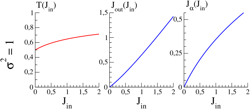
Figure 2: (Color online) Dependencies of the transmission coefficient, $T$, the outgoing light intensity, ${\cal J}_{\text{out}}$, and the resonator’s mode intensity, ${\cal J}_{\alpha}$, on the incoming light intensity, ${\cal J}_{\text{in}}$, for $\sigma^{2}(\omega)=1$ and negative product $(\sigma(\omega)\cdot{\cal J}_{\alpha})$.

It follows from Eqs. (6) and (9) that the nonlinear transmission problem is completely determined by the value of $\sigma(\omega)$ and the sign of the product $\sigma(\omega)\cdot{\cal J}_{\alpha}$. As is illustrated in Fig. 2, for frequencies where $(\sigma(\omega)\cdot{\cal J}_{\alpha})<0$, the transmission coefficient $T$ and the outgoing light intensity ${\cal J}_{\text{out}}$ grow monotonically with ${\cal J}_{\text{in}}$ for all values of $\sigma(\omega)$.

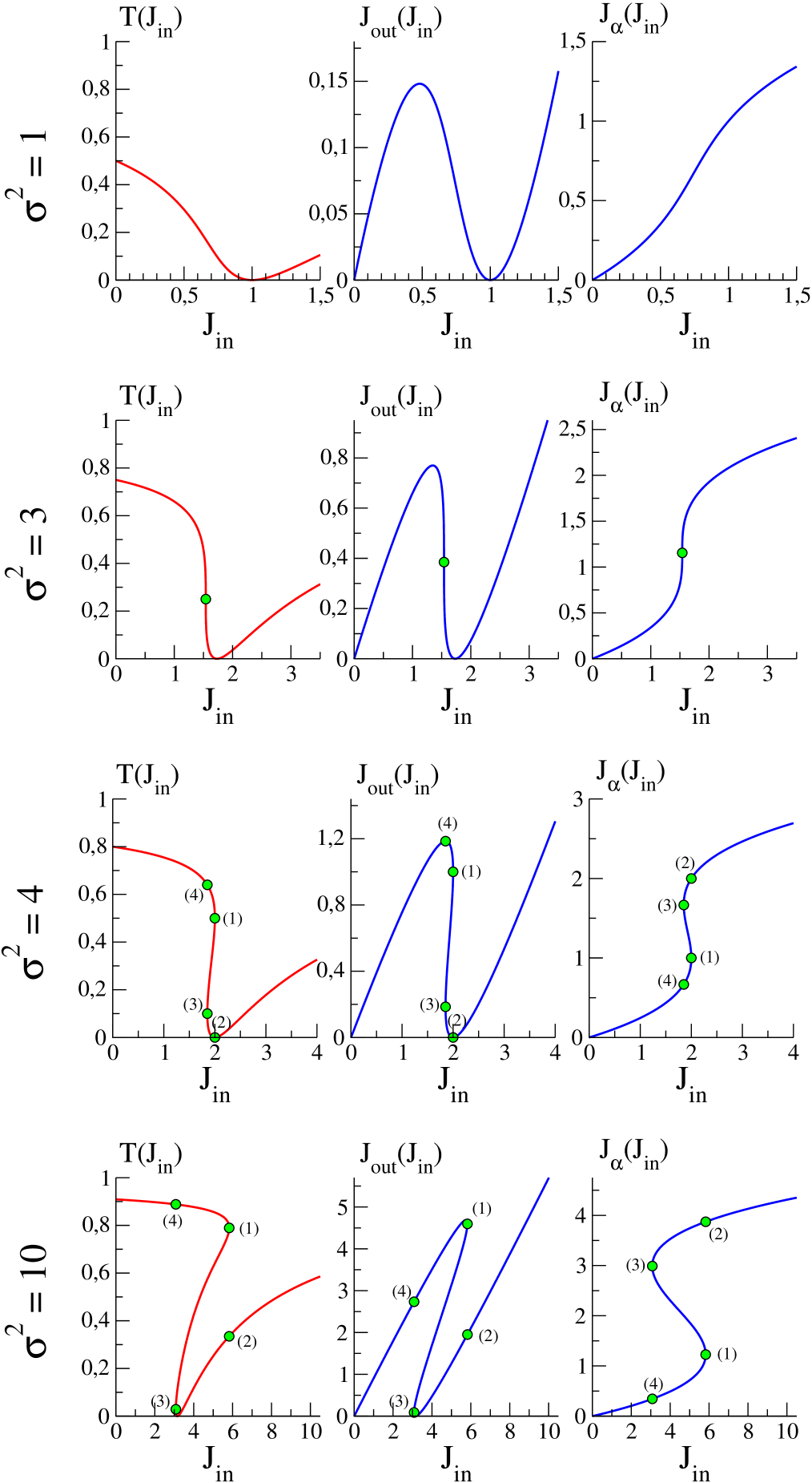
Figure 3: (Color online) Dependencies of the transmission coefficient, $T$, the outgoing light intensity, ${\cal J}_{\text{out}}$, and the resonator’s mode intensity, ${\cal J}_{\alpha}$, on the incoming light intensity, ${\cal J}_{\text{in}}$, for several different values of $\sigma^{2}(\omega)$ and positive product $(\sigma(\omega)\cdot{\cal J}_{\alpha})$.

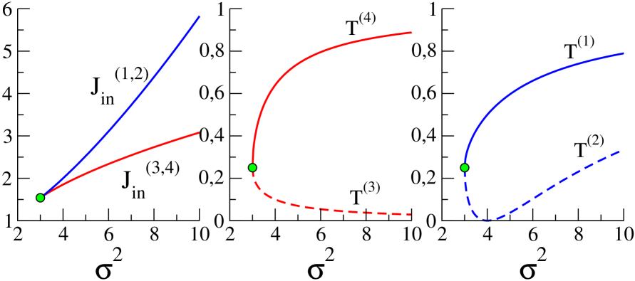
Figure 4: (Color online) Dependencies of the threshold incoming light intensity and the corresponding transmission coefficients on $\sigma^{2}(\omega)$ for the four critical points (1)-(4) indicated by circles in Fig. 3. Here, we assume that $(\sigma(\omega)\cdot{\cal J}_{\alpha})>0$.

The situation becomes more interesting for frequencies lying on the other side of the resonance where $(\sigma(\omega)\cdot{\cal J}_{\alpha})>0$. In this case $T$ and, therefore, ${\cal J}_{\text{out}}$ become non-monotonic functions of ${\cal J}_{\text{in}}$, as is illustrated in Fig. 3. Moreover, for $\sigma^{2}(\omega)>3$ these functions become multi-valued functions of ${\cal J}_{\text{in}}$ in the interval ${\cal J}_{\text{in}}^{(3,4)}\leq{\cal J}_{\text{in}}\leq{\cal J}_{\text{in}}^{(1,2)}$, where

$${\cal J}_{\text{in}}^{(1,2)}=\frac{2}{27}\left\{\sigma^{3}+9\sigma+\left[\sigma^{2}-3\right]^{3/2}\right\}\;,$$

$${\cal J}_{\text{in}}^{(3,4)}=\frac{2}{27}\left\{\sigma^{3}+9\sigma-\left[\sigma^{2}-3\right]^{3/2}\right\}\;,$$ (12)

which are also shown in Fig. 4. In this interval the nonlinear light transmission becomes bistable: low- and high-transmission regimes coexist at the same value of the incoming light intensity ${\cal J}_{\text{in}}$, as can be seen in Fig. 3 for $\sigma^{2}>3$ (intermediate parts of the curves correspond to unstable transmission). Therefore, by increasing an intially low intensity ${\cal J}_{\text{in}}$ we obtain a hysteris where we jump from the point (1) to (2), and then upon decreasing ${\cal J}_{\text{in}}$, we jump from the point (3) to (4). The transmission coefficients at these characteristic points are

$$T^{(1,3)} = \frac{1}{2\sigma^{2}(1\mp\sqrt{1-3/\sigma^{2}})-2}\;,$$

$$T^{(2,4)} = \frac{(1\mp 2\sqrt{1-3/\sigma^{2}})^{2}}{5-3/\sigma^{2}\mp 4\sqrt{1-3/\sigma^{2}}}\;,$$ (13)

and they are depicted in Fig. 4. For completeness, we also present the expressions for the resonator’s mode intensity at these points

$${\cal J}_{\alpha}^{(1,3)} = \frac{2\sigma}{3}\mp\frac{1}{3}\sqrt{\sigma^{2}-3}\;,$$

$${\cal J}_{\alpha}^{(2,4)} = \frac{2\sigma}{3}\pm\frac{2}{3}\sqrt{\sigma^{2}-3}\;.$$ (14)

From a practical point of view, these solutions have important consequences. Firstly, the bistability condition $\sigma^{2}>3$ corresponds to a linear transmission $T>3/4$. That is, the bistable transmission becomes possible only for frequencies where $(\sigma(\omega)\cdot{\cal J}_{\alpha})$ is positive and linear transmission exceeds 75%. As demonstrated in Fig. 4 and Eq. (II.2), when $\sigma^{2}$ grows, all threshold intensities grow, too, starting with the minimum threshold intensity ${\cal J}_{\text{in}}^{(1,2,3,4)}=8/3^{1.5}\approx 1.54$ at $\sigma^{2}=3$.

For ideal nonlinear switching the coefficients $T^{(1)}$ and $T^{(4)}$ should be close to unity while $T^{(2)}$ and $T^{(3)}$ should vanish. However, as can be seen from Fig. 4 and the asymptotic (for large $\sigma^{2}$) expressions

$$T^{(1)} \approx 1-\frac{9}{\sigma^{2}}\;,\quad T^{(2)}\approx 1-\frac{9}{4\sigma^{2}}\;,$$

$$T^{(3)} \approx 1-\frac{1}{\sigma^{2}}\;,\quad T^{(4)}\approx\frac{1}{4\sigma^{2}}\;,$$ (15)

of Eqs. (II.2), these conditions cannot be satisfied simultaneously. In particular, the transmission coefficient $T^{(2)}$ does not vanish but approaches unity for large $\sigma^{2}$. Moreover, there exists no condition under which $T^{(2)}$ and $T^{(3)}$ vanish simultaneously. Therefore, it is impossible to create ideal nonlinear switches in these systems.

A reasonable compromise for realistic nonlinear switching schemes of this type could be the usage of the frequency with $\sigma^{2}\simeq 5$, for which the linear light transmission is close to $83\%$. For this case, the critical transmission coefficients $T^{(2)}\simeq 3.7\%$ and $T^{(3)}\simeq 7\%$ are sufficiently small, while $T^{(1)}\simeq 60\%$ and $T^{(4)}\simeq 74\%$ are large enough for practical purposes. The threshold intensities ${\cal J}_{\text{in}}^{(1,2)}\simeq 2.53$ and ${\cal J}_{\text{in}}^{(3,4)}\simeq 2.11$ differ about 20% from each other, so that in this case one can achieve a high-contrast and robust switching for sufficiently small modulation of the incoming power.

The above analysis suggests that the optimal dimensionless threshold intensities are fixed around ${\cal J}_{\text{in}}^{(i)}\sim 2.5$ so that the real threshold power of the incoming light, $P_{\text{in}}^{(i)}=P_{0}{\cal J}_{\text{in}}^{(i)}$, can only be minimized by minimizing the characteristic power, $P_{0}$, of the system. An inspection of Eq. (11) shows that this can be facilitated by increasing the resonator nonlinear feedback parameter, $\kappa_{\alpha}$, the material nonlinearity, $\chi^{(3)}_{\alpha}$, or the resonator quality factor, $Q$. For small-volume photonic crystal resonators, it has been established that $\kappa\sim 0.2$ (see Yanik:2003-2739:APL ; Soljacic:2002-55601:PRE ), and this value can hardly be further increased.

Therefore, only two practical strategies remain that could lead to an enhancement of nonlinear effects in this system. The first approach is based on specific material properties: We should create the resonator $\alpha$ from a material with the largest possible value of $\chi^{(3)}_{\alpha}$. In high-index semiconductors, nearly instantaneous Kerr nonlinearity reaches values of $n_{2}\sim 1.5\times 10^{-13}$ cm²/W Sheik-Bahae:1991-1296:IQE , where $n_{2}\propto\chi^{(3)}/n_{0}$ and $n_{0}$ is the linear refractive index of the material. Even such relatively weak nonlinearity is already sufficient for many experimental observations of the bistability effect in the waveguide-resonator systems Notomi:2005-2678:OE ; Barclay:2005-801:OE . However, using polymers with nearly instantaneous Kerr nonlinearity of the order of $n_{2}>10^{-11}$ cm²/W and, at the same time, sufficiently weak two-photon absorption Samoc:1995-1241:OL , one could potentially decrease the value of $P_{0}$ by at least two orders of magnitude. Polymers, however, have a low refractive index which is insufficient for creating a (linear) photonic bandgap required to obtain good waveguiding and low losses. The solution to this could be the embedding of such highly nonlinear but low-index materials into a host photonic crystal made of a high-index semiconductor. Optimized waveguding designs for the basic functional devices of this kind are available  Mingaleev:2004-2858:OL ; Schillinger:2005-324:SPIE ; Jiao:2005-1875:IPTL and recent experimental progress Heijden:2006-161112:APL ; Ferrini:2006-1238:OL may soon allow a realization of corresponding linear and nonlinear devices.

The second approach is based on designing waveguide-resonator structures with the largest possible quality factor, $Q$. Potentially, one can increase $Q$ indefinitely by mere increase of the distance between the waveguide and the resonator. However, this leads to a corresponding increase in the size of the nonlinear photonic devices. A very attractive alternative possibility for increasing $Q$ is based on the adjustment of the resonator geometry Akahane:2003-944:NAT .

In what follows, we suggest yet another possibility to dramatically increase $Q$ through an optimal choice of the resonator location relative to the discrete locations of the cavities that form the photonic-crystal waveguide.

II.3 Limitations of the coupled-mode theory

Standard coupled-mode theory exhibits a number of limitations. Firstly, it gives analytical expression for the detuning parameter $\sigma(\omega)$ only near the resonator frequency $\omega_{\alpha}$. And this immediately highlights the second limitation: standard coupled-mode theory Xu:2000-7389:PRE ; Yanik:2003-2739:APL ; Soljacic:2002-55601:PRE ; Cowan:2003-46606:PRE ; Cowan:2005-R41:SST ; Chak:2006-035105:PRE cannot analytically describe resonant effects near waveguide band edges. However, numerical studies Waks:2005-5064:OE have recently demonstrated that the effects of the waveguide dispersion become very important at the band edges and may lead to non-Lorentzian transmission spectra in coupled waveguide-resonator systems.

As a matter of fact, the question “what happens if the resonator frequency $\omega_{\alpha}$ lies near the edge of the waveguide passing band or even outside it?” may be of a great practical importance due to two reasons. Firstly, in realistic structures it is not always possible to appropriately tune the frequency $\omega_{\alpha}$, and therefore it is important to understand properties of the system for any location of the resonance frequency. Secondly, as we have already mentioned in the Introduction, PhC waveguides can provide us with a very slow group velocity of the propagating pulses — but in most cases they do it exactly at the passing band edges. Therefore, if we wish to utilize such a slow light propagation for nonlinearity enhancement, we should extend the above analysis to such cases, too.

In what follows, we describe an alternative analytical approach to the coupled waveguide-resonator structures which allows us to correctly analyze both linear and nonlinear transmission for arbitrary locations of the resonator frequency $\omega_{\alpha}$ relative to the waveguide passing band, including the transmission near band edges in the slow light regime.

III Discrete model approach

Having discussed the results obtained for the continuous-waveguide structure shown in Fig. 1(a), we now take into account the discrete nature of the waveguding structure embedded in photonic crystals. In particular, we analyze what will change in the system properties when we move the resonator along the waveguide from the on-site location shown in Fig. 1(b) to the inter-site location shown in Fig. 1(c). Our analysis is based on effective discrete equations that have been derived for the description of photonic crystal devices McGurn:1999:PLA ; Mingaleev:2000-5777:PRE ; Mingaleev:2001-5474:PRL ; Mingaleev:2002-2241:JOSB ; Mingaleev:2002-231:OL in combination with a recently developed discrete model approach to nonlinear Fano resonances Miroshnichenko:2005-36626:PRE .

III.1 Discrete Equation Approach

First, we derive an appropriate set of discrete equations [see Eqs. (III.1) below], and show that they can be applied to a variety of the photonic-crystal devices. We start from the wave equation in the frequency domain for the electric field

$$\left[\vec{\nabla}\times\vec{\nabla}\times-\left(\frac{\omega}{c}\right)^{2}\hat{\varepsilon}(\vec{r})\right]\vec{E}(\vec{r})=0\;,$$ (16)

where the dielectric function $\hat{\varepsilon}(\vec{r})=\hat{\varepsilon}_{\text{pc}}(\vec{r})+\delta\hat{\varepsilon}(\vec{r})$ consists of the dielectric function $\hat{\varepsilon}_{\text{pc}}(\vec{r})$ of a perfectly periodic structure and a perturbation $\delta\hat{\varepsilon}(\vec{r})$ that describes the embedded cavities. It is convenient to introduce the tensorial Green function of the perfectly periodic photonic crystal,

$$\left[\vec{\nabla}\times\vec{\nabla}\times-\left(\frac{\omega}{c}\right)^{2}\hat{\varepsilon}_{\text{pc}}(\vec{r})\right]\hat{G}(\vec{r},\vec{r}\,^{\prime}|\omega)=\hat{I}\delta(\vec{r}-\vec{r}\,^{\prime})$$ (17)

and to rewrite Eq. (16) in the integral form,

$$\vec{E}(\vec{r})=\left(\frac{\omega}{c}\right)^{2}\int\vec{r}\,^{\prime}\;\hat{G}(\vec{r},\vec{r}\,^{\prime}|\omega)\,\delta\hat{\varepsilon}(\vec{r}\,^{\prime})\,\vec{E}(\vec{r}\,^{\prime})\;,$$ (18)

where we assume that the frequency $\omega$ lies inside a complete photonic bandgap so that the electric field vanishes everywhere except for areas inside and in the vicinity of cavities. We enumerate the cavities by an integer index $n$ and introduce dimensionless functions $\theta_{n}(\vec{r})$ which describe the shape of the $n$-th cavity. As a result, $\delta\hat{\varepsilon}(\vec{r})$ may be represented as

$$\delta\hat{\varepsilon}(\vec{r})=\sum_{n}\left[\delta\hat{\varepsilon}_{n}+\chi^{(3)}_{n}|\vec{E}(\vec{r})|^{2}\right]\theta_{n}(\vec{r}-\vec{R}_{n})\;,$$ (19)

where $\vec{R}_{n}$, $\delta\hat{\varepsilon}_{n}$, and $\chi^{(3)}_{n}$ are, respectively, position, (linear) dielectric function, and nonlinear third-order susceptibility of the $n$-th cavity.

Similar to Sec. II, we describe the electric field of the $n$-th cavity mode via a dimensionless field profile $\vec{{\cal E}}_{n}(\vec{r})$ and a complex amplitude $A_{n}$. Taking into account that inside the cavities the electric field of the system is a superposition

$$\vec{E}(\vec{r})\simeq\sum_{n}A_{n}\,\vec{{\cal E}}_{n}(\vec{r}-\vec{R}_{n})\;,$$ (20)

Eq. (18) can be rewritten as a set of discrete nonlinear equations

$$D_{n}(\omega)A_{n}=\sum_{m\neq n}V_{n,m}(\omega)A_{m}+\kappa_{n}(\omega)\chi^{(3)}_{n}|A_{n}|^{2}A_{n},$$ (21)

where $D_{n}(\omega)=1-V_{n,n}(\omega)$ is the dimensionless frequency detuning from the resonance frequency, $\omega_{n}$, of the $n$-th cavity. Furthermore,

$$V_{n,m}(\omega) = \frac{\delta\varepsilon_{m}}{W_{n}}\left(\frac{\omega}{c}\right)^{2}\!\int\!d\vec{r}\!\int\!d\vec{r}\,^{\prime}\;\vec{{\cal E}}^{*}_{n}(\vec{r})\hat{\varepsilon}_{n}(\vec{r})$$

$$\times \theta_{m}(\vec{r}\,^{\prime})\hat{G}(\vec{r}+\vec{R}_{n}-\vec{R}_{m},\vec{r}\,^{\prime}|\omega)\,\vec{{\cal E}}_{m}(\vec{r}\,^{\prime})\;,$$

is the dimensionless linear coupling between the $n$-th and the $m$-th cavity. Similarly,

$$\kappa_{n}(\omega) = \frac{1}{W_{n}}\left(\frac{\omega}{c}\right)^{2}\!\int\!d\vec{r}\!\int\!d\vec{r}\,^{\prime}\;\vec{{\cal E}}^{*}_{n}(\vec{r})\hat{\varepsilon}_{n}(\vec{r})$$

$$\times \theta_{n}(\vec{r}\,^{\prime})\hat{G}(\vec{r},\vec{r}\,^{\prime}|\omega)\,|\vec{{\cal E}}_{n}(\vec{r}\,^{\prime})|^{2}\vec{{\cal E}}_{n}(\vec{r}\,^{\prime})\;,$$

is the dimensionless and scale-invariant nonlinear feedback parameter which should be compared with the analogous parameter (8) introduced in the conventional coupled-mode theory analysis Soljacic:2002-55601:PRE ; Yanik:2003-2739:APL . Finally, $W_{n}$ is defined in exactly the same way as $W_{\alpha}$ in Eq. (II.1).

We remark that in deriving Eqs. (21) we have neglected higher-order couplings proportional to the integrals of $\vec{{\cal E}}^{*}_{n}(\vec{r})\vec{{\cal E}}_{m}(\vec{r}+\vec{R}_{n}-\vec{R}_{m})$ with $n\neq m$ but take into account the coupling coefficients which involve integrals of $\hat{G}(\vec{r}+\vec{R}_{n}-\vec{R}_{m},\vec{r}\,^{\prime}|\omega)$ with $n\neq m$. This approximation is sufficiently accurate in most cases, as we demonstrate in Refs. Mingaleev:2002-231:OL ; Miroshnichenko:2005-3969:OE . We would like to mention that in Eqs. (21)–(III.1) we have used more accurate definitions of the coupling coefficients than those that have been introduced earlier in Refs. McGurn:1999:PLA ; Mingaleev:2000-5777:PRE ; Mingaleev:2001-5474:PRL ; Mingaleev:2002-231:OL . They have also a more generic form than those we used in Ref. Mingaleev:2002-2241:JOSB .

Typical frequency dependencies of the parameters of the discrete model, Eq. (21), are displayed in Figs. 9–11 of Appendix A, where we also discuss the application of Eqs. (21)–(III.1) to simple structures such as linear and nonlinear photonic crystal resonators and straight waveguides. Here, we apply Eqs. (21)–(III.1) to study the more complicated case of the nonlinear coupled waveguide-resonator systems shown in Figs. 1(b,c). The set of Eqs. (21) may be separated in this case according to

$$D_{\text{w}}(\omega)A_{n} = \sum_{j=1}^{L}V_{j\text{w}}(\omega)(A_{n+j}+A_{n-j})+V_{n,\alpha}(\omega)A_{\alpha}\;,$$

$$D_{\alpha}(\omega)A_{\alpha} = \sum_{j}V_{\alpha,j}(\omega)A_{j}+\kappa_{\alpha}(\omega)\chi^{(3)}_{\alpha}|A_{\alpha}|^{2}A_{\alpha}\;,$$ (24)

where we assume that all cavities of the photonic-crystal waveguide are identical and linear, so that we can denote $D_{\text{w}}(\omega)\equiv D_{n}(\omega)$ and $V_{j\text{w}}(\omega)\equiv V_{n,n\pm j}(\omega)$ for any $n$ inside the waveguide. Furthermore, the index $\alpha$ defines the parameters of the side-coupled nonlinear resonator. Below we show that the assumption of linear waveguide cavities may be relaxed for frequencies near the resonator resonance frequency $\omega_{\alpha}$ because then the amplitudes $A_{n}$ remain small in comparison with the amplitude $A_{\alpha}$.

For the first equation in Eq. (III.1), we seek solutions of standard form

$$A_{n}=\begin{cases}\;I_{\text{in}}^{1/2}\,t(\omega)\,e^{ik(\omega)sn}&\!\!\text{for $n\gg 1$},\\ \;I_{\text{in}}^{1/2}\,\Bigl{[}e^{ik(\omega)sn}+r(\omega)\,e^{-ik(\omega)sn}\Bigr{]}&\!\!\text{for $n\ll-1$},\\ \end{cases}$$ (25)

where $s$ is the distance between the nearest waveguide cavities and $I_{\text{in}}$ is the intensity of the incoming light. For both structures shown in Figs. 1(b,c), we obtain that the transmission and reflection coefficients can formally be described by the same expressions (1)–(2) as for the structure depicted in Fig. 1(a). However, within the discrete equation approach the expression for the detuning parameter $\sigma(\omega)$ can now be found for the entire frequency range. Below, we discuss novel results for the structures shown in Fig. 1(b) and Fig. 1(c) separately.

III.2 On-site resonator

First, we obtain the solution of this problem for the structure shown in Fig. 1(b). For simplicity, we assume that the only nonvanishing coupling coefficients in Eq. (III.1) are $V_{1\text{w}}(\omega)$, $V_{\alpha,0}(\omega)$, and $V_{0,\alpha}(\omega)$ (see, however, Appendix B for a more accurate analysis which takes into account additional coupling coefficients). As a result, we obtain the transmission and reflection coefficients described by Eqs. (1)–(2) with $\phi_{r}=\pi/2$ and a corresponding expression for $\sigma(\omega)$:

$$\sigma(\omega)=2\sin\left[k(\omega)s\right]\,\frac{V_{1\text{w}}(\omega)}{V_{0,\alpha}(\omega)}\frac{A_{0}}{A_{\alpha}}\;,$$ (26)

which should be considered as a generalized intensity-dependent frequency detuning parameter $\sigma(\omega)+{\cal J}_{\alpha}$ introduced in Eq. (6) above. The amplitude $A_{0}$ in Eq. (26) is given by

$$A_{0} = t(\omega)\,I_{\text{in}}^{1/2}\;,$$ (27)

while the waveguide dispersion relation $k(\omega)$ is determined by Eq. (48).

In the case of a linear $\alpha$-resonator (i.e. $\chi^{(3)}_{\alpha}\equiv 0$), the amplitude $A_{\alpha}=V_{\alpha,0}(\omega)A_{0}/D_{\alpha}(\omega)$ is proportional to the amplitude $A_{0}$. Therefore, $\sigma(\omega)$ and, accordingly, the transmission and reflection coefficients do not depend on the light intensity. Upon introducing the abbreviation

$$\mu(\omega)=\frac{D_{\alpha}(\omega)V_{1\text{w}}(\omega)}{V_{0,\alpha}(\omega)V_{\alpha,0}(\omega)}\;,$$ (28)

the detuning parameter, Eq. (26), for a linear $\alpha$-resonator reads as

$$\sigma(\omega)=2\mu(\omega)\sin\left[k(\omega)s\right]\;.$$ (29)

This implies that $\sigma(\omega)$ vanishes when either $D_{\alpha}(\omega)=0$ or $k(\omega)=\pi n/s$ with an arbitrary integer $n$. The first condition reproduces Eq. (3) with $\omega_{\text{res}}=\omega_{\alpha}$ and the resonance width $\gamma$ given by

$$\gamma\approx\frac{\omega_{\alpha}\Delta_{\alpha}}{\sin[k(\omega_{\alpha})s]}\approx\frac{s\,\omega_{\alpha}\omega_{\text{w}}}{v_{\text{gr}}}\,\nu_{\alpha}\,\nu_{\text{w}}\,V_{0,\alpha}V_{\alpha,0}\;,$$ (30)

where $\nu_{\alpha}$ and $\nu_{\text{w}}$ are defined by Eq. (43),

$$\Delta_{\alpha}=\frac{V_{0,\alpha}V_{\alpha,0}}{2\omega_{\alpha}D^{\prime}_{\alpha}V_{1\text{w}}}=\frac{V_{0,\alpha}V_{\alpha,0}}{2V_{1\text{w}}}\,\nu_{\alpha}\;,$$ (31)

and the group velocity

$$v_{\text{gr}}=\left.\frac{d\omega}{dk}\right|_{\omega_{\alpha}}\approx-2s\,\omega_{\text{w}}\nu_{\text{w}}V_{1\text{w}}\sin[k(\omega_{\alpha})s]\;,$$ (32)

can be found directly from Eq. (48). Here and in what follows, we assume that the values of all frequency-dependent parameters whithout explicitly stated frequency dependence are evaluated at the resonance frequency, $\omega_{\text{res}}$. Finally, we notice that the resonance width, Eq. (30), is very similar to that described by the coupled-mode theory, Eq. (4).

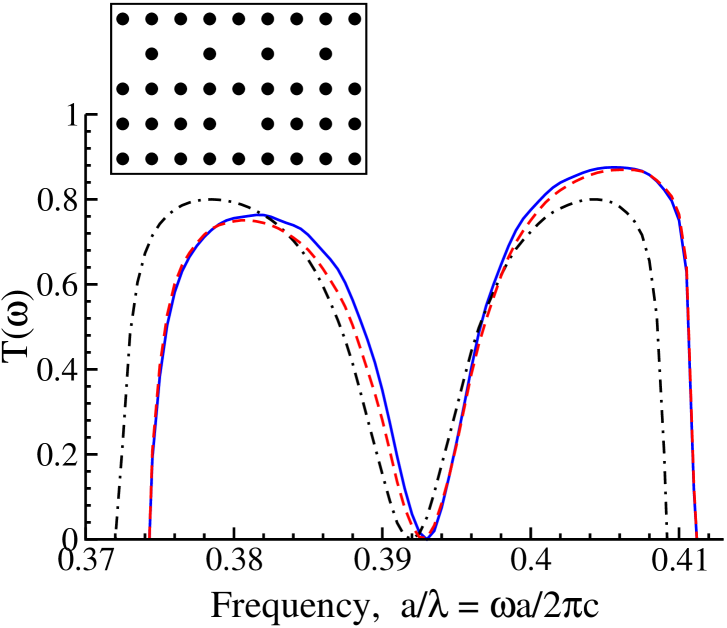
Figure 5: (Color online) Linear transmission through a photonic crystal waveguide that is created by removing every second rod in a row ($\vec{s}=2\vec{a}_{1}$) side-coupled to a one-site resonator created by removing a single rod. The underlying 2D photonic crystal is described in Appendix A.1. We compare exact numerical results (solid line) with the analytical results based on Eq. (29) (dot-dashed line) and Eq. (50) (dashed line).

It is important that the quality factor $Q$ of the resonance

$$Q=\frac{\omega_{\alpha}}{2\gamma}\approx\frac{\sin\left[k(\omega_{\alpha})s\right]}{2\Delta_{\alpha}}\approx\frac{v_{\text{gr}}}{s\,\omega_{\text{w}}}\,\frac{1}{2\,\nu_{\alpha}\nu_{\text{w}}\,V_{0,\alpha}V_{\alpha,0}}\;,$$ (33)

is multiplied by the factor $\sin\left[k(\omega_{\alpha})s\right]\sim v_{\text{gr}}$, and, therefore, becomes strongly suppressed near the edges of waveguide passing band, $k(\omega_{\alpha})=0,\,\pm\pi/s$. Accordingly, the detuning parameter (29) vanishes at these edges, too. This means that, in agreement with the numerical calculations shown in Fig. 5, the transmission coefficient $T(\omega)$ vanishes not only at the resonance frequency, but also at both edges of the waveguide passing band. Such an effect was recently observed by Waks and Vukovic Waks:2005-5064:OE in their numerical calculations based on standard coupled-mode theory which takes into account the waveguide dispersion. Therefore, the effect of vanishing transmission at the spectral band edges may be attributed also to the structure shown in Fig. 1(a).

Obviously, this enhancement of light scattering at the waveguide band edges should be very important from the point of view of fabrication tolerances since virtually any imperfection contributes to scattering losses. Moreover, as discussed in Sec. IV, this effect is detrimental to the concept of all-optical switching devices based on slow-light photonic crystal waveguides.

We support this conclusion by another observation. First, the light intensity at the $0$-th cavity, $|A_{0}|^{2}=T(\omega)I_{\text{in}}$, vanishes at the resonance frequency for arbitrary large incoming light intensity, because $T(\omega_{\alpha})\equiv 0$. Therefore, the nonlinearity of this cavity may safely be neglected. In contrast, the light intensity at the $\alpha$-resonator reaches its maximum value at $\omega_{\alpha}$,

$$|A_{\alpha}(\omega_{\alpha})|^{2}\simeq 4\left(\frac{V_{1\text{w}}}{V_{0,\alpha}}\right)^{2}\sin^{2}[k(\omega_{\alpha})s]\cdot I_{\text{in}}$$

$$\simeq\left(\frac{v_{\text{gr}}}{s\omega_{\text{w}}\,\nu_{\text{w}}V_{0,\alpha}}\right)^{2}\cdot I_{\text{in}}\simeq\left(2Q\,\nu_{\alpha}V_{\alpha,0}\right)^{2}\cdot I_{\text{in}}\;,$$ (34)

which may significantly exceed the incoming light intensity $I_{\text{in}}$ when the coupling $V_{0,\alpha}$ between the $\alpha$-resonator and waveguide becomes small enough relative to the coupling $V_{1\text{w}}$ between the cavities in the waveguide. This strong enhancement suggests a physical explanation for the existence of the rather strong nonlinear effect of light bistability at relatively low intensities of the incoming light. However, when the resonance frequency $\omega_{\alpha}$ lies close to any of the waveguide band edges, it is seen from Eq. (III.2) that the light intensity at the $\alpha$-resonator becomes (strongly) suppressed by a factor $\sin^{2}[k(\omega_{\alpha})s]$ .

Details of an extension of the above discussion to the case of more realistic non-local couplings, i.e., more than nearest neighbors couplings, is presented in Appendix B and here we only summarize the results. Both, a non-locality of the inter-coupling between waveguide cavities as well as a nonlocality of cross-coupling with the $\alpha$-resonator lead to a small shift in the resonance frequency, $\omega_{\text{res}}$, but do not change the main result about the suppression of the detuning $\sigma(\omega)$ and transmission $T(\omega)$ at both edges of the waveguide passing band. However, we would like to emphasize that for a fully quantitative analysis, non-local couplings have to be taken into account, for instance, within the framework of the recently developed Wannier function approach Busch:2003-R1233:JPCM .

We now consider the case when the resonator $\alpha$ is nonlinear, i.e. $\chi^{(3)}_{\alpha}\neq 0$. As has been previously shown in Ref. Miroshnichenko:2005-36626:PRE , this case, too, can be studied analytically even for non-local couplings between the cavities and resonator and novel effects originating solely from the non-locality may be expected when the non-local coupling strength exceeds one half of the local coupling. Unfortunately, in realistic photonic crystals this limit may hardly be realized so that here we restrict our analysis to the local-coupling approximation. In this case, we obtain from the second equation in Eqs. (III.1) that the amplitude $A_{\alpha}$ uniquely determines the amplitude $A_{0}$. Substituting the latter expression into Eqs. (26)–(27), we find that the nonlinear transmission is described by Eqs. (6) and (9) with the detuning $\sigma(\omega)$ determined by Eqs. (28)–(29) and the dimensionless intensities ${\cal J}_{\alpha}$ and ${\cal J}_{\text{in}}$ given by the expressions

$${\cal J}_{\alpha} \simeq 2Q\kappa_{\alpha}\nu_{\alpha}\chi^{(3)}_{\alpha}|A_{\alpha}|^{2}\;,$$ (35)

$${\cal J}_{\text{in}} \simeq 8\sin[k(\omega_{\text{res}})s]\,V_{1\text{w}}\left(\frac{\delta\varepsilon_{0}}{\delta\varepsilon_{\alpha}}\right)Q^{2}\kappa_{\alpha}\nu_{\alpha}^{2}\chi^{(3)}_{\alpha}I_{\text{in}}$$

$$\simeq -\frac{4v_{\text{gr}}}{s\,\omega_{\text{w}}}\left(\frac{\delta\varepsilon_{0}\nu_{\alpha}}{\delta\varepsilon_{\alpha}\nu_{\text{w}}}\right)Q^{2}\kappa_{\alpha}\nu_{\alpha}\chi^{(3)}_{\alpha}I_{\text{in}}\;,$$

where $Q$ is determined by Eq. (33). Therefore, all the results for the nonlinear light transmission which are displayed in Figs. 2–4 are directly applicable to the structure of Fig. 1(b), too.

In an experiment, one measures not the light intensity in the waveguide, $I_{\text{in}}$, but the propagation power, Eq. (10), where for the discrete structure of Fig. 1(b), the characteristic power $P_{0}$ is

$$P_{0} \simeq \frac{c^{2}k(\omega_{\alpha})}{16\pi\sin[k(\omega_{\alpha})s]\omega_{\alpha}V_{1\text{w}}}\left(\frac{\delta\varepsilon_{\alpha}}{\delta\varepsilon_{0}}\right)\frac{1}{Q^{2}\kappa_{\alpha}\nu_{\alpha}^{2}\chi^{(3)}_{\alpha}}$$ (36)

$$\simeq -\frac{c^{2}k(\omega_{\alpha})s}{8\pi v_{\text{gr}}}\left(\frac{\omega_{\text{w}}\delta\varepsilon_{\alpha}\nu_{\text{w}}}{\omega_{\alpha}\delta\varepsilon_{0}\nu_{\alpha}}\right)\frac{1}{Q^{2}\kappa_{\alpha}\nu_{\alpha}\chi^{(3)}_{\alpha}}\;.$$

Again, this result is quite similar to Eq. (11) for the continuous structure of Fig. 1(a). Nevertheless, our more general analysis explicitly suggests that it should be better to use the $\alpha$-resonator with the resonance frequency at the center of the waveguide passing band $k(\omega_{\alpha})\approx\pi/2s$, where the group velocity reaches its maximum. Notice, however, that this suggestion becomes wrong for the structure of Fig. 1(c) studied in the next subsection.

III.3 Inter-site resonator

In the system where the $\alpha$-resonator is placed symmetrically between two cavities of the waveguide and, therefore, couples equally to both of them, a qualitatively different type of resonant transmission occurs. The corresponding structure is schematically shown in Fig. 1(c). Assuming that in this case the nonvanishing coupling coefficients in Eq. (III.1) are $V_{1\text{w}}(\omega)$, $V_{\alpha,1}(\omega)\equiv V_{\alpha,0}(\omega)$, and $V_{1,\alpha}(\omega)\equiv V_{0,\alpha}(\omega)$, we seek solutions to the first equation of the system (III.1) that are of the form of Eq. (25). Again, we find that the transmission and reflection coefficients are given by Eqs. (1)–(2) albeit with the frequency-dependent phase $\phi_{r}(\omega)=\pi/2+k(\omega)s$. Here, $k(\omega)$ is determined by Eq. (48), and the generalized intensity-dependent frequency detuning is

$$\sigma(\omega)+{\cal J}_{\alpha}=i-i\left(e^{ik(\omega)s}-1\right)\frac{V_{1\text{w}}(\omega)}{V_{0,\alpha}(\omega)}\frac{I_{\text{in}}^{1/2}}{A_{\alpha}}\;.$$ (37)

The corresponding amplitudes are

$$A_{0} = I_{\text{in}}^{1/2}-\frac{1}{[1-e^{-ik(\omega)s}]}\frac{V_{0,\alpha}(\omega)}{V_{1\text{w}}(\omega)}A_{\alpha}\;,$$

$$A_{1} = e^{ik(\omega)s}I_{\text{in}}^{1/2}-\frac{1}{[1-e^{-ik(\omega)s}]}\frac{V_{0,\alpha}(\omega)}{V_{1\text{w}}(\omega)}A_{\alpha}\;.$$ (38)

Despite the complex form of Eq. (37), we would like to emphasize that the detuning $\sigma(\omega)$ determined by Eq. (37) is a real-valued function (see also the discussion following Eq. (1) above).

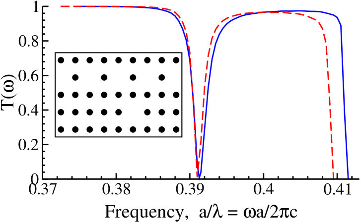
Figure 6: (Color online) Liner transmission through a photonic crystal waveguide created by removing every second rod in a row ($\vec{s}=2\vec{a}_{1}$) side-coupled to an inter-site resonator created by removing a single rod. The underlying 2D photonic crystal described in Appendix A.1. We compare exact numerical results (solid line) with the analytical results based on Eq. (39) (dashed line).

In the case of the linear $\alpha$-resonator (i.e., for $\chi^{(3)}_{\alpha}\equiv 0$), we obtain

$$\sigma(\omega) = \left[1+\mu(\omega)\right]\tan\left(\frac{k(\omega)s}{2}\right)\;,$$ (39)

where $\mu(\omega)$ is given by Eq. (28). For a high-quality $\alpha$-resonator in the vicinity of the resonance frequency this detuning parameter can be approximated by Eq. (3) with $\omega_{\text{res}}\simeq\omega_{\alpha}\left(1-2\Delta_{\alpha}\right)$ and

$$\gamma = \frac{2\omega_{\text{res}}\Delta_{\alpha}}{\tan[k(\omega_{\text{res}})s/2]}\;.$$ (40)

Here, $\Delta_{\alpha}$ is defined by Eq. (31). In contrast to Eq. (33), the corresponding quality factor

$$Q=\frac{\omega_{\text{res}}}{2\gamma}\approx\frac{\tan\left[k(\omega_{\text{res}})s/2\right]}{4\Delta_{\alpha}}\approx\frac{V_{1\text{w}}\tan\left[k(\omega_{\text{res}})s/2\right]}{2\,\nu_{\alpha}\,V_{0,\alpha}V_{\alpha,0}}$$ (41)

is now multiplied by the factor $\tan[ks/2]$ which does not vanish and even diverges as $k(\omega_{\text{res}})$ approaches the edge of the transmission band $k=\pm\pi/s$. At this band edge, $\sigma(\omega)\sim\tan(k(\omega)s/2)\to\infty$ and, therefore, light transmission is always perfect. This conclusion is supported by the exact numerical calculations presented in Fig. 6. At the other band edge, i.e., for $k(\omega)=0$, transmission vanishes, similar to the structures shown in Figs. 1(a,b).

The light intensity at the $\alpha$-resonator reaches its maximal value at the resonance frequency

$$|A_{\alpha}(\omega_{\text{res}})|^{2} \simeq 4\left(\frac{V_{1\text{w}}}{V_{0,\alpha}}\right)^{2}\sin^{2}\left[\frac{k(\omega_{\text{res}})s}{2}\right]\cdot I_{\text{in}}$$ (42)

$$\simeq \left(4Q\nu_{\alpha}V_{\alpha,0}\cos\left[\frac{k(\omega_{\text{res}})s}{2}\right]\right)^{2}\cdot I_{\text{in}}\;$$

Again, in contrast to the corresponding light intensity (III.2) for the on-site coupled structure, Eq. (42) does not vanish at the edge of the transmission band $k=\pm\pi/s$. Therefore, we can expect that for inter-site coupled structure nonlinear effects at the band edge $k=\pm\pi/s$ should be sufficiently strong to allow bistable transmission and switching.

To investigate this, we assume that the $\alpha$-resonator is nonlinear ($\chi^{(3)}_{\alpha}\neq 0$) and introduce the same dimensionless intensities ${\cal J}_{\alpha}$ and ${\cal J}_{\text{in}}$ as in Eq. (35). However, now the quality factor $Q$ is defined by Eq. (41) and the resonance frequency is $\omega_{\text{res}}\simeq\omega_{\alpha}(1-2\Delta_{\alpha})$. We find that this nonlinear problem, too, has a solution of the form given by Eqs. (6) and (9). However, now the detuning $\sigma(\omega)$ is given by Eq. (39). Therefore, all results presented above in Figs. 2–4 remain applicable to this structure, too. The only but very important qualitative difference of the structure shown in Fig. 1(c) is that the transmission coefficient $T(\omega)$ and the corresponding light intensity $|A_{\alpha}|^{2}$ at the $\alpha$-resonator do not vanish at the band edge $k=\pm\pi/s$ since the quality factor $Q$ at this band edge grows to infinity for the inter-site structure of Fig. 1(c). Therefore, this structure may be utilized for realizing efficient all-optical switching devices based on slow-light photonic crystal waveguides. This is in sharp contrast to the structures shown in Figs. 1(a,b).

IV Discussion of results

In this section, we summarize our results and emphasize their importance by applying them to specific photonic-crystal structures. We consider a two-dimensional photonic crystal created by a square lattice of dielectric rods in air. The rods are made from $Si$ or $GaAs$ ($\varepsilon=11.56$) and have radius $r=0.18a$.

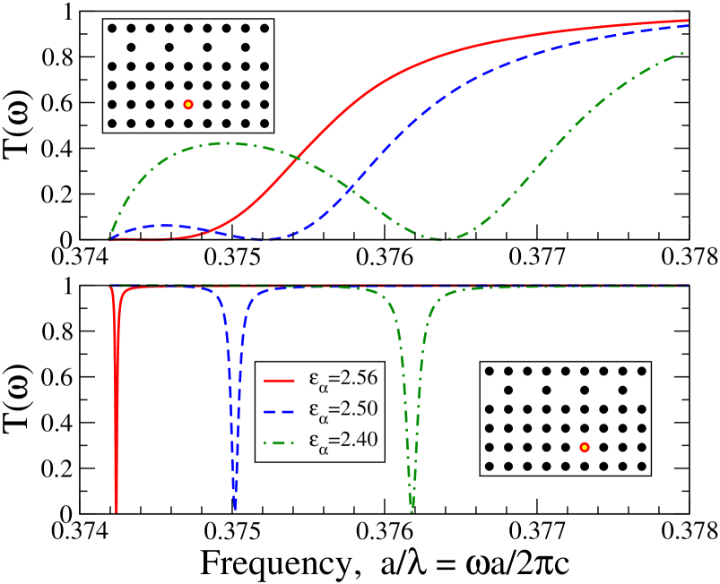
Figure 7: (Color online) Linear transmission spectrum for a photonic crystal waveguide created by removing every second rod in a row ($\vec{s}=2\vec{a}_{1}$) side-coupled to a single on-site (a) or inter-site (b) polymer-rod resonator (marked by the open circle in the insets). The underlying 2D photonic crystal is described in Appendix A.1 and results for three different values of the resonator dielectric constant $\varepsilon_{\alpha}$ are shown.

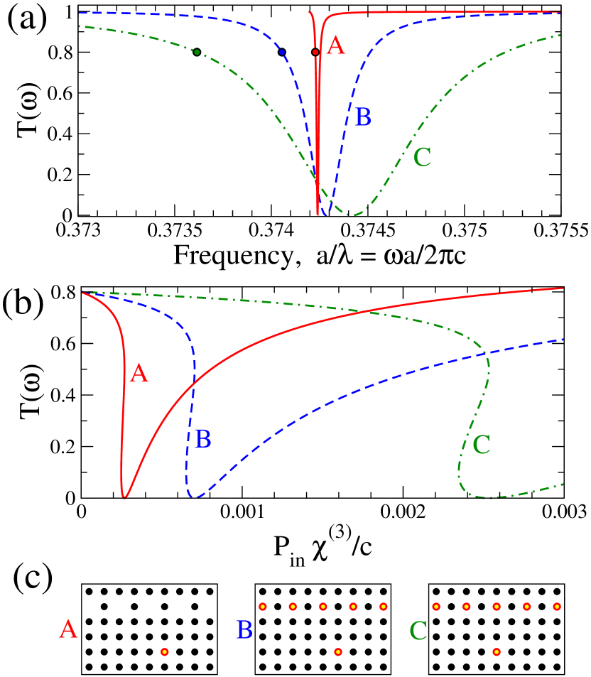
Figure 8: (Color online) (a) Linear transmission spectrum and (b) nonlinear bistable transmission for three different side-coupled waveguide-resonator photonic crystal structures whose topology is shown in (c). The rods consist of Si or GaAs (full black circles) or polymer (open red circles). Example A represents a close to optimal structure with inter-site location of the $\alpha$-resonator whose resonance frequency lies close to the edge $k=\pm\pi/s$ of the passing band; example B represents a sub-optimal structure with an inter-site location of the $\alpha$-resonator whose resonance frequency lies near the center of the passing band; example C represents a sub-optimal but commonly used structure with an on-site location of the $\alpha$-resonator whose resonance frequency lies near the center of the passing band. Closed circles in (a) indicate frequencies with $T(\omega)=80\%$ that are used for achieving high-contrast bistability in (b). Red circles in (c) indicate positions of the nonlinear polymer rods with $\varepsilon_{\alpha}=2.56$. Other parameters of the 2D photonic crystal are described in Appendix A.1.

First, we consider a waveguide created by removing every second rod ($s=2a$) in a straight line of rods coupled to a nonlinear resonator $\alpha$ created by replacing a single rod of the two-dimensional lattice with a highly-nonlinear polymer rod. The corresponding structure is schematically shown in the insets in Fig. 7. The resonant frequency of the polymer-rod resonator lies very close to the edge $k=\pm\pi/s$ of the waveguide passing band, and can be tuned by changing the linear dielectric constant $\varepsilon_{\alpha}$ of the rod.

In Fig. 7(a) and (b), respectively, we display the transmission spectra for both on-site and inter-site positions of the side-coupled resonator for three different values of resonator dielectric constant $\varepsilon_{\alpha}$. We notice that in the case of the on-site position of the resonator the transmission coefficient $T(\omega)$ remains below the critical value of $T=75\%$ required for bistable switching operation for all frequencies $\omega$ below the resonance frequency $\omega_{\text{res}}$. The condition $\omega<\omega_{\text{res}}$ corresponds to the condition $(\sigma(\omega)\cdot{\cal J}_{\alpha})>0$ which should be satisfied to realize nonmonotonic dependencies of the nonlinear transmission shown in Fig. 4). Therefore, this on-site system cannot exhibit bistability.

On the other hand, bistability may be realized for the inter-site position of the side-coupled resonator for which, in a full agreement with our analysis presented above, the transmission remains perfect at the band edge $k=\pm\pi/s$ and the quality factor $Q$ increases as the resonant frequency approaches this band edge. In Fig. 8(b) (example A) we show that in this case bistable transmission indeed occurs for the frequency marked by a filled circle in Fig. 8(a). This corresponds to $T(\omega)=80\%$, i.e., the choice $\sigma^{2}(\omega)=4$ for the detuning parameter.

We want to emphasize that the large value of the quality factor (41) for the inter-site structure at $k(\omega)$ close to $\pm\pi/s$ leads to very low bistability thresholds as compared to the cases of on-site coupled and continous waveguide coupled structures. This is illustrated in examples B and C of Fig. 8: Relative to the waveguide design in example A, the design in example B moves the resonance frequency deeper into the passing band thus decreasing the quality factor (41). Nevertheless, the inter-site coupled example B still exhibits a much smaller bistability threshold than the on-site coupled system with the same waveguide design in example C. This is caused by (usually) much smaller waveguide-resonator coupling and, accordingly, much larger $Q$ in the inter-site structures as compared to the on-site structures.

Summarizing, the inter-site structure of the resonant waveguide-resonator interaction schematically shown in Fig. 1(c) allows to achieve much higher values for the linear quality factor $Q$. As a consequence, much smaller bistability threshold intensities for the nonlinear transmission are obtained. To employ these advantages, the wavevector $k(\omega_{\text{res}})$ of the guided mode at the resonance frequency $\omega_{\text{res}}$, Eq. (39), should be as close as possible to $\pi/s$. This requirement coincides with the condition of a very small group velocity in the waveguide and, in contrast to the continuous-waveguide and on-site structures depicted in Figs. 1(a,b), provides us with a possibility to create low-threshold all-optical switching devices based on slow-light photonic crystal waveguides.

V Conclusions

We have presented a detailed analysis of PhC waveguides side-coupled to Kerr nonlinear resonators which may serve as a basic element of active photonic-crystal circuitry. First, we have extended the familiar approach based on standard coupled-mode theory and derived explicit analytical expressions for the bistability thresholds and transmission coefficients related to light switching in such structures. Our results reveal that, from the point of view of bistability contrast (a small difference between two threshold intensities and robustness of switching) the best conditions for bistability are realized for those parameter values for which the dimensionless detuning parameter $\sigma(\omega)$ is close to $\sqrt{5}$. Practically, this corresponds to the choice of operation frequencies for which the linear light transmission is close to 83%.

We have pointed out that the conventional coupled-mode theory does not allow to describe the light transmission near the band edges, and we have developed an improved semi-analytical approach based on the effective discrete equations derived in the framework of a consistent Green’s function formalism. This approach is ideally suited for a qualitative and semi-quantitative description of photonic-crystal devices that involve a discrete set of small-volume cavities. We have shown that this novel approach allows to adequately describe light transmission in the waveguide-resonator structures near the band edges. Specifically, we have demonstrated that while the transmission coefficient vanishes at both spectral edges for the on-site coupled structure (see Fig. 1(b)), light transmission remains perfect at one band edge for the inter-site coupled structure (see Fig. 1(c)). These features allow a significant enhancement of the resonator quality factor and, accordingly, a substantial reduction of the bistability threshold. As a consequence, we refer to this type of nonlinearity enhancement as a geometric enhancement. The possibility of such enhancement is a direct consequence of the discreteness of the photonic crystal waveguide and is in a sharp contrast to similar resonant systems based on ridge waveguides. The potential of this novel type of the nonlinearity enhancement may be regarded as an additional argument to support the application of photonic-crystal devices in integrated photonic circuits.

In addition, we would like to emphasize that the engineering of the geometry of photonic-crystal based devices such as that presented in Fig. 1(c) becomes extremely useful for developing novel concepts of all-optical switching in the slow-light regime of PhC waveguides which may have much wider applications in nanophotonics and is currently under active experimental research Vlasov-slow-light .

We believe that the basic concept of the geometric enhancement of nonlinear effects based on the discrete nature of photonic-crystal waveguides will be useful in the study of more complicated devices and circuits and, in particular, for various slow-light applications. For instance, this concept may be applied to the transmission of a side-coupled resonator placed between two partially reflecting elements embedded into the photonic-crystal waveguide where sharp and asymmetric line shapes have been predicted with associated variations of the transmission from 0% to 100% over narrow frequency ranges Fan:2002-908:APL . Similarly, the concept can be extended to a system of cascaded cavities Lin:2005-165330:PRB and three-port channel-drop filters Kim:2004-5518:OE , optical delay lines Wang:2003-66616:PRE , systems of two nonlinear resonators with a very low bistability threshold Maes:2005-1778:JOSB , etc.

Appendix A Calculation of the model parameters and examples

A.1 Coupling coefficients for two-dimensional photonic crystals

To obtain deeper insight into the basic properties of the effective discrete equations (21), we should know how the coupling coefficients $D_{n}(\omega)$, $\kappa_{n}(\omega)$, and $V_{n,m}(\omega)$ depend on frequency $\omega$. As an illustration, we consider a two-dimensional model of a photonic crystal consisting of a square lattice (lattice spacing $a$) of infinitely long dielectric rods (see Refs.  Fan:1998-960:PRL ; Soljacic:2002-55601:PRE ; Yanik:2003-2739:APL and also references [7-16] in Ref. Mingaleev:2002-2241:JOSB ). We study light propagation in the plane of periodicity, assuming that the rods have a radius $r=0.18a$ and a dielectric constant of $\varepsilon_{\text{rod}}=11.56$ (GaAs or Si at the telecommunication wavelength $\lambda\sim 1.55$ $\mu$m). For light with the electric field polarized along the rods ($E$-polarized light), this photonic crystal exhibits a large (38% of the center frequency) photonic bandgap that extends from $\omega=0.303\,(2\pi c/a)$ to $\omega=0.444\,(2\pi c/a)$

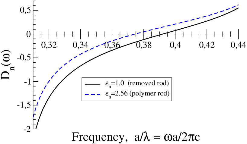
Figure 9: (Color online) Frquency dependence of the detuning coefficient $D_{n}(\omega)$ for the 2D photonic crystal described in Appendix A.1, for two types of resonators: Removing a single rod ($\varepsilon_{n}=1.0$; solid line) leads to a localized mode at $\omega_{n}=0.392$, while replacing a single rod by a geometrically identical rod made of polymer ($\varepsilon_{n}=2.56$, dashed line) leads to a localized mode at $\omega_{n}=0.374$.

Our task is to evaluate the coupling coefficients $D_{n}(\omega)$, $\kappa_{n}(\omega)$, and $V_{n,m}(\omega)$ using Eqs. (III.1)–(III.1) with the Green’s function $\hat{G}(\vec{r},\vec{r}\,^{\prime}|\omega)$ calculated by the method described earlier in Refs. Mingaleev:2000-5777:PRE ; Mingaleev:2001-5474:PRL . The results of these calculations are displayed in Figs. 9–11.

A.2 Isolated optical resonators

For the case of an isolated ($V_{n,m}=0$) linear ($\chi^{(3)}_{n}=0$) optical resonator at the site $n$, Eq. (21) takes a simplest possible form, $D_{n}(\omega)A_{n}=0$. In this case, we only need to know the dimensionless frequency detuning coefficient, $D_{n}(\omega)$. In Fig. 9 we plot $D_{n}(\omega)$ for two types of resonators: a resonator created by removing a single rod and a resonator created by replacing a single rod with a polymer rod of the same radius and $\varepsilon_{n}=2.56$. Introducing the dimensionless frequency $\tilde{\omega}=a/\lambda\equiv(\omega a/2\pi c)$, we can express these coefficients, with a very good accuracy in the range $0.36\leq\tilde{\omega}\leq 0.41$, by the following cubic dependencies: $D_{n}(\omega)=9.426(\tilde{\omega}-\tilde{\omega}_{\text{n}})-10.889(\tilde{\omega}-\tilde{\omega}_{\text{n}})^{2}+840.36(\tilde{\omega}-\tilde{\omega}_{\text{n}})^{3}$ with $\tilde{\omega}_{\text{n}}=0.3919$, for the removed rod, and $D_{n}(\omega)=9.047(\tilde{\omega}-\tilde{\omega}_{\text{n}})-49.555(\tilde{\omega}-\tilde{\omega}_{\text{n}})^{2}+770.14(\tilde{\omega}-\tilde{\omega}_{\text{n}})^{3}$ with $\tilde{\omega}_{\text{n}}=0.3744$, for the replaced rod.

The resonator mode can only be excited at the resonator frequency $\omega_{n}$, which is determined by the equation $D_{n}(\omega_{n})=0$. Fig. 9 suggests that changing the dielectric constant of the resonator $\varepsilon_{n}$ allows to tune the frequency $\omega_{n}$. In all cases, in the vicinity of the resonator frequency $\omega_{n}$, the coupling coefficient $D_{n}(\omega)$ can be approximately expanded into the Taylor series with a linear dependence

$$D_{n}(\omega)\simeq\frac{\omega-\omega_{n}}{\nu_{n}\,\omega_{n}}\;,\quad\nu_{n}=\frac{1}{\omega_{n}D_{n}^{\prime}(\omega_{n})}\;,$$ (43)

where we have introduced a dimensionless parameter $\nu_{n}$ which describes the resonator sensitivity to a change of the dielectric constant. For our example of a polymer-rod resonator, we find $\nu_{n}\approx 0.295$.

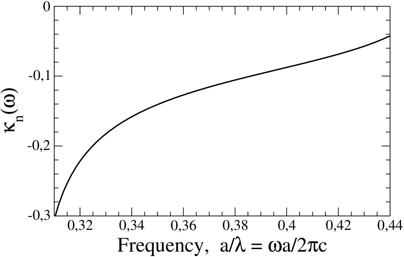
Figure 10: Frequency dependence of the nonlinear feedback parameter $\kappa_{n}(\omega)$ for the 2D photonic crystal described in Appendix A.1. The nonlinear resonator is created by replacing a single rod with a polymer rod of the same radius which supports at $\varepsilon_{n}=2.56$ a localized mode with frequency $\omega_{n}=0.374$.

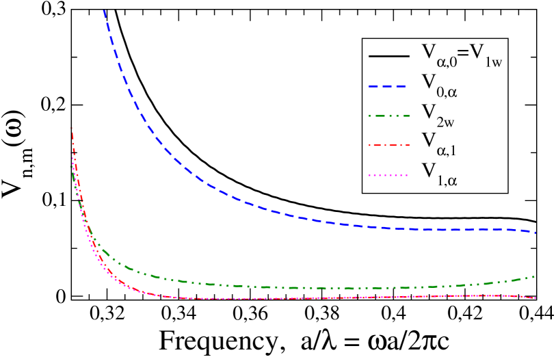
Figure 11: (Color online) Frequency dependence of the coupling coefficients $V_{n,m}(\omega)$ for the 2D photonic crystal described in Appendix A.1 with a on-site side-coupled waveguide-resonator system shown in Fig. 1-b. The notations are the same as those in Eq. (III.1) and we assume that the waveguide is created by removing every second rod in a row (located at $\vec{R}_{n}=2\vec{a}_{1}n$) whereas the on-site resonator is created by replacing a single rod at $\vec{R}_{\alpha}=-2\vec{a}_{2}$ with a polymer rod ($\varepsilon_{n}=2.56$) of the same radius. The dispersion relation for such a waveguide is displayed in Fig. 12.

When the $n$-th resonator is nonlinear (i.e., $\chi^{(3)}_{n}\neq 0$), Eq. (21) reduces to the equation $D_{n}(\omega)A_{n}=\kappa_{n}(\omega)\chi^{(3)}_{n}|A_{n}|^{2}A_{n}$ with the new important coefficient — nonlinear feedback parameter $\kappa_{n}(\omega)$. In Fig. 10, we depict the frequency dependence of $\kappa_{n}(\omega)$ for the case of a nonlinear polymer resonator. In the frequency range $0.36\leq\tilde{\omega}\leq 0.41$, this behavior can be approximated as $\kappa_{n}(\omega)=-0.111+1.005(\tilde{\omega}-\tilde{\omega}_{\text{n}})-5.501(\tilde{\omega}-\tilde{\omega}_{\text{n}})^{2}+85.57(\tilde{\omega}-\tilde{\omega}_{\text{n}})^{3}$ with $\tilde{\omega}_{\text{n}}=0.3744$. Therefore, in the vicinity of the resonator’s frequency, $\omega_{n}$, we may assume that $\kappa_{n}(\omega)\approx-0.111$ is constant and can rewrite Eq. (21) according to

$$|A_{n}|^{2}=\frac{D_{n}(\omega)}{\kappa_{n}(\omega)\chi^{(3)}_{n}}\approx\frac{D_{n}^{\prime}(\omega_{n})}{\kappa_{n}(\omega_{n})\chi^{(3)}_{n}}(\omega-\omega_{n}).$$ (44)

The solution of the above equation gives us the dependence of the resonator frequency $\omega_{\text{res}}$ on the resonator’s mode intensity $|A_{n}|^{2}$ as

$$\omega_{\text{res}}\approx\omega_{n}\left(1+\kappa_{n}\nu_{n}\,\chi^{(3)}_{n}\,|A_{n}|^{2}\right)\;.$$ (45)

Here, we have used the notation $\kappa_{n}=\kappa_{n}(\omega_{n})$. As we see, the nonlinear sensitivity of the resonator at the site $n$ is a product of its nonlinear feedback parameter, $\kappa_{n}$, the sensitivity to a change of the dielectric constant, $\nu_{n}$, and the Kerr susceptibility of material, $\chi^{(3)}_{n}$. The sign of this product defines the direction of the resonator frequency shift. In particular, for the polymer resonator used in Figs. 9–10, we obtain a rather small shift, $\kappa_{n}\nu_{n}\approx-0.033$ which indicates that for $\chi^{(3)}_{n}>0$ the resonator frequency decreases as the light intensity grows. Designing optical resonators with larger $\kappa_{n}$ or $\nu_{n}$, may allow to enhance their nonlinear properties for a given material with Kerr nonlinearity $\chi^{(3)}_{n}$.

A.3 Straight waveguides

Now let us consider an array of identical coupled cavities separated by the distance $s=|\vec{s}|$ which create a straight photonic-crystal waveguide depicted in Figs. 1(b,c). Before proceeding, we would like to emphasize that our analysis can equally well be applied to the coupled-resonator optical waveguides (CROWs) suggested in Ref. Yariv:1999-711:OL . If we neglect nonlinear effects (assuming that either the waveguide cavities are linear, $\chi^{(3)}_{n}=0$, or the light intensity in the waveguide remains sufficiently small), Eq. (21) reduces to

$$D_{\text{w}}(\omega)A_{n}=\sum_{j=1}^{\infty}V_{j\text{w}}(\omega)(A_{n+j}+A_{n-j})\;.$$ (46)

Here we have defined, similar to Eq. (III.1), $D_{\text{w}}(\omega)\equiv D_{n}(\omega)$ and $V_{j\text{w}}(\omega)\equiv V_{n,n\pm j}(\omega)$ which are identical for all $n$.

In Fig. 11 we plot the frequency dependencies of $V_{1\text{w}}(\omega)$ and $V_{2\text{w}}(\omega)$ for a photonic-crystal waveguide created by removing every second rod in a row, either with $\vec{s}=2\vec{a}_{1}$ or with $\vec{s}=2\vec{a}_{2}$. In the vicinity of the polymer-rod resonator frequency, the coupling coefficients are to lowest order constant: $V_{1\text{w}}\approx 0.096$ and $V_{2\text{w}}\approx 0.0086$ . In the general case, our calculations show that the coefficients $V_{j\text{w}}(\omega)$ decay nearly exponentially with $j$. In terms of frequency, they take on a constant value at the central passing band frequency and grow rapidly towards the low-frequency bandgap edge.

According to the Floquet-Bloch theorem, Eq. (46) has a solution $A_{n}=A_{0}\exp[\pm ik(\omega)sn]$ with an arbitrary complex amplitude $A_{0}$. The corresponding dispersion $k(\omega)$ is determined by the equation

$$D_{\text{w}}(\omega)=\sum_{j=1}^{L}2V_{j\text{w}}(\omega)\cos\left[k(\omega)s\,j\right]\;,$$ (47)

where we assume that the coupling coefficients $V_{j\text{w}}(\omega)$ vanish for all $j$ above $L$. As a matter of fact, our studies indicate that sufficiently accurate results can be obtained already for $L\sim 4a/s$. In Fig. 12 we plot the dispersion relation for a 2D model photonic-crystal waveguide and compare it with exact numerical results calculated by the super-cell plane-wave method Johnson:2001-173:OE . For this case, even the simplest tight-binding approximation (i.e., at $L=1$) gives quite satisfactory results.

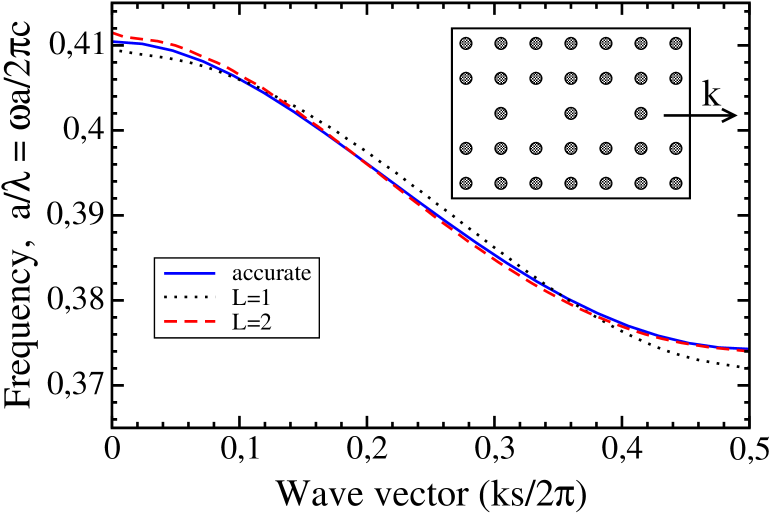
Figure 12: (Color online) Dispersion relation for a photonic crystal waveguide created by removing every second rod in a row ($\vec{s}=2\vec{a}_{1}$) in the 2D photonic crystal described in Appendix A.1. Numerical exact results (solid line) are calculated with the super-cell plane-wave method Johnson:2001-173:OE and the approximate results are obtained from Eq. (47) with $L=1$ (dotted line) and $L=2$ (dashed line), using the coupling coefficients from Fig. 11.

In the tight-binding approximation ($L=1$) the dispersion relation can be described by the following simple expression

$$\cos\left[k(\omega)s\right]=\frac{D_{\text{w}}(\omega)}{2V_{1\text{w}}(\omega)}\simeq\frac{\omega-\omega_{\text{w}}}{\omega_{\text{w}}\Delta_{\text{w}}}\;,$$ (48)

where $\omega_{\text{w}}$ is the resonance frequency of the waveguide cavities. Furthermore, we have the dimensionless parameter

$$\Delta_{\text{w}}=\frac{2V_{1\text{w}}(\omega_{\text{w}})}{\omega_{\text{w}}D^{\prime}_{\text{w}}(\omega_{\text{w}})}=2V_{1\text{w}}\nu_{\text{w}}\;,$$ (49)

with $V_{1\text{w}}\equiv V_{1\text{w}}(\omega_{\text{w}})$ and $\nu_{\text{w}}$ defined by Eq. (43), that equals half-bandwidth of the waveguide transmission band. This band extends from $\omega_{\text{w}}(1-\Delta_{\text{w}})$ to $\omega_{\text{w}}(1+\Delta_{\text{w}})$. For our example of photonic crystal waveguide, we find $\Delta_{\text{w}}\approx 0.052$, i.e., its bandwidth is about $10\%$.

Appendix B Effect of long-range interactions

B.1 Effects of nonlocal dispersion

As follows from the results of Sec. III.2 above, the local-coupling approximation provides us with an excellent qualitative analysis of the structure shown in Fig. 1(b). However, certain physically important effects may be missed in this approximation. A detailed analysis of the effects of nonlocal coupling was performed in Ref. Miroshnichenko:2005-36626:PRE , so that here we may discuss this issue very briefly, and may specify it directly to photonic-crystal devices.

In Fig. 5, we provide a comparison of $T(\omega)$ calculated from Eq. (29) in the local-coupling approximation with the exact numerical results for the structure shown in Fig. 1(b) for the model photonic crystal described in Appendix A.1. The results suggest that the local-coupling approximation introduces a frequency shift for the band edges which agrees well with the corresponding frequency shift in the dispersion relation shown in Fig. 12.

In addition, the resonance frequency is also shifted; it is not equal to $\omega_{\alpha}$ but is slightly larger. In principle, this shift can be produced by two effects: (i) a long-range coupling between cavities inside the waveguide and (ii) a long-range coupling between the waveguide and the side-coupled resonator. First, we explore the former possibility.

Solving Eqs. (III.1)–(25) for $L=2$, we obtain the transmission and reflection coefficients (1)–(2) with the detuning parameter

$$\sigma(\omega)=2\sin(ks)\,\cdot\frac{D_{\alpha}\left[V_{1\text{w}}^{3}+3D_{\text{w}}V_{1\text{w}}V_{2\text{w}}+3V_{1\text{w}}V_{2\text{w}}^{2}+2V_{2\text{w}}^{3}\cos(3ks)\right]-V_{0,\alpha}V_{\alpha,0}V_{1\text{w}}V_{2\text{w}}}{V_{0,\alpha}V_{\alpha,0}\left(V_{1\text{w}}^{2}-V_{2\text{w}}^{2}+D_{\text{w}}V_{2\text{w}}\right)}\;,$$ (50)

where all the coefficients are assumed to be frequency-dependent analogous to Eqs. (28)-(29). The waveguide dispersion $k(\omega)$ is now calculated from Eq. (47) with $L=2$.

Fig. 5 shows that the transmission calculated from Eq. (50) is much closer to the exact numerical results. In fact, the nominator of Eq. (50) indicates that, indeed, the resonance frequency is slightly shifted from the value $\omega_{\alpha}$, and that this shift is proportional to $V_{2\text{w}}$. Since $V_{2\text{w}}$ is always much smaller than $V_{1\text{w}}$ (see Fig. 11), we can safely neglect all the terms proportional to $V_{2\text{w}}^{n}$ with $n\geq 2$, and obtain the resonance frequency according to

$$\omega_{\text{res}}\approx\omega_{\alpha}\left(1+\frac{V_{0,\alpha}V_{\alpha,0}V_{1\text{w}}V_{2\text{w}}}{(V_{1\text{w}}^{3}+3D_{\text{w}}V_{1\text{w}}V_{2\text{w}})}\,\nu_{\alpha}\right)\;.$$ (51)

Here, the values of all coefficients are calculated at the frequency $\omega_{\alpha}$, and $\nu_{\alpha}$ is defined by Eq. (43).

In addition to the shift of the resonance frequency, a perfect transmission may occur at the frequencies for which the denominator in Eq. (50) vanishes:

$$V_{2\text{w}}=V_{1\text{w}}\left(\frac{\cos(ks)\pm\sqrt{1+\cos^{2}(ks)-2\cos(2ks)}}{1-2\cos(2ks)}\right)\;.$$ (52)

However, an analysis reveal that Eq. (52) has solutions only when $|V_{2\text{w}}(\omega)|$ exceeds $|V_{1\text{w}}(\omega)|/2$, a condition that appears to be impossible to realize in realistic photonic crystals.

B.2 Effects of nonlocal coupling

Another possible reason for a shift of the resonance frequency is a nonlocal coupling between the waveguide cavities and the side-coupled resonator $\alpha$. Here, we discuss this effect in the framework of the tight-binding approximation for the waveguide dispersion (i.e., $L=1$) to distinguish it from the other type of nonlocal effects discussed in the previous sub-section. We assume that $V_{j,\alpha}(\omega)=V_{\alpha,j}(\omega)=0$ for all $j\geq 2$, and take into account that, for the symmetric structure shown in Fig. 1(b), the coupling coefficients are: $V_{-1,\alpha}(\omega)\equiv V_{1,\alpha}(\omega)$ and $V_{\alpha,-1}(\omega)\equiv V_{\alpha,1}(\omega)$. Then, we obtain a solution of Eqs. (III.1)–(25) in the form of Eqs. (1)–(2) with the detuning parameter defined as

$$\sigma(\omega)=2\sin[ks]\,\cdot\frac{D_{\alpha}V_{1\text{w}}+V_{0,\alpha}V_{\alpha,1}+V_{\alpha,0}V_{1,\alpha}+2V_{\alpha,1}V_{1,\alpha}\cos(ks)}{\bigl{[}V_{\alpha,0}+2V_{\alpha,1}\cos(ks)\bigr{]}\bigl{[}V_{0,\alpha}+2V_{1,\alpha}\cos(ks)\bigr{]}}\;.$$ (53)

Here, all coefficients are assumed to be frequency-dependent, similar to Eqs. (28)-(29). Furthermore, the waveguide dispersion $k(\omega)$ is calculated again from Eq. (48).

Eq. (53) suggests that in this case the resonance frequency becomes slightly shifted from the value $\omega_{\alpha}$, and this shift is proportional to the values of $V_{1,\alpha}$ and $V_{\alpha,1}$, which for our example (see Fig. 5) are equal to $V_{\alpha,1}=-0.0026$ and $V_{1,\alpha}=-0.0022$. Assuming that these coupling coefficients are always much smaller than $V_{0,\alpha}$ and $V_{\alpha,0}$ (cf. $V_{\alpha,0}=0.096$ and $V_{0,\alpha}=0.082$), we obtain for the resonance frequency

$$\omega_{\text{res}}\approx\omega_{\alpha}\left(1-\frac{V_{0,\alpha}V_{\alpha,1}+V_{\alpha,0}V_{1,\alpha}}{V_{1\text{w}}}\,\nu_{\alpha}\right)\;.$$ (54)

Here, the coefficients are calculated at the resonance frequency $\omega_{\alpha}$, and $\nu_{\alpha}$ is defined by Eq. (43). For the example shown in Fig. 5, this frequency shift is much smaller than that described by Eq. (51) because in this case the values of $V_{\alpha,1}$ and $V_{1,\alpha}$ are 3.3 times smaller than the value of $V_{2\text{w}}$.

Due to this long-range coupling, there appears a possibility of perfect light transmission, as discussed in Ref. Miroshnichenko:2005-36626:PRE , but only in the case when $|V_{\alpha,1}(\omega)|$ exceeds $|V_{\alpha,0}(\omega)|/2$ or $|V_{1,\alpha}(\omega)|$ exceeds $|V_{0,\alpha}(\omega)|/2$. Again, such a scenario appears to be impossible to realize in realistic photonic crystal structures.

References

- (1) H.M. Gibbs, Optical bistability: Controlling light with light (Academic Press, Orlando, 1985).
- (2) K. Busch, S. Lölkes, R.B. Wehrspohn, and H. Föll (Eds.), Photonic Crystals: Advances in Design, Fabrication, and Characterization (Wiley-VCH, Berlin, 2004); K. Inoue and K. Ohtaka (Eds.), Photonic Crystals: Physics, Fabrication and Applications (Springer, Berlin, 2004).
- (3) S. Noda, A. Chutinan, and M. Imada, Nature 407, 608 (2000).
- (4) A. Chutinan, M. Mochizuki, M. Imada, and S. Noda, Appl. Phys. Lett. 79, 2690 (2001).
- (5) T. Asano, B. S. Song, Y. Tanaka, and S. Noda, Appl. Phys. Lett. 83, 407 (2003).
- (6) M. Imada, S. Noda, A. Chutinan, M. Mochizuki, and T. Tanaka, J. Lightwave Techn. 20, 873 (2002)
- (7) C.J.M. Smith et al., Appl. Phys. Lett. 78, 1487 (2001).
- (8) C. Seassal et al., IEEE J. Quantum Electron. 38, 811 (2002).
- (9) M. Notomi et al., Opt. Express 13, 2678 (2005).
- (10) P.E. Barclay, K. Srinivasan, and O. Painter, Opt. Express 13, 801 (2005).
- (11) H.A. Haus, Waves and Fields in Optoelectronics, (Prentice Hall, Englewood Cliffs, NJ, 1984).
- (12) H. A. Haus and Y. Lai, IEEE J. Quantum Electron. 28, 205 (1992).
- (13) U. Fano, Phys. Rev. 124, 1866 (1961).
- (14) P. W. Anderson, Phys. Rev. 124, 41 (1961).
- (15) S. H. Fan, P. R. Villeneuve, and J. D. Joannopoulos, Phys. Rev. Lett. 80, 960 (1998).
- (16) Y. Xu, Y. Li, R. K. Lee, and A. Yariv, Phys. Rev. E 62, 7389 (2000).
- (17) M. Soljacic, M. Ibanescu, S. G. Johnson, Y. Fink, and J. D. Joannopoulos, Phys. Rev. E 66, 055601(R) (2002).
- (18) M. F. Yanik, S. H. Fan, and M. Soljacic, Appl. Phys. Lett. 83, 2739 (2003).
- (19) P. Chak, S. Pereira, and J. E. Sipe, Phys. Rev. B 73, 035105 (2006).
- (20) A. R. Cowan and J. F. Young, Phys. Rev. E 68, 046606 (2003).
- (21) A. R. Cowan and J. F. Young, Semicond. Sci. Technol. 20, R41 (2005).
- (22) A. E. Miroshnichenko, S. F. Mingaleev, S. Flach, and Yu. S. Kivshar, Phys. Rev. E 71, 036626 (2005).
- (23) A. E. Miroshnichenko and Yu. S. Kivshar, Phys. Rev. E 72, 056611 (2005).
- (24) A. E. Miroshnichenko and Yu. S. Kivshar, Opt. Express 13, 3969 (2005).
- (25) S.F. Mingaleev and Yu.S. Kivshar, J. Opt. Soc. Am. B 19, 2241 (2002).
- (26) S. F. Mingaleev and Yu. S. Kivshar, Opt. Lett. 27, 231 (2002).
- (27) A. R. McGurn, Phys. Lett. A 251, 322 (1999); Phys. Lett. A 260, 314 (1999).
- (28) S. F. Mingaleev, Yu. S. Kivshar, and R. A. Sammut, Phys. Rev. E 62, 5777 (2000).
- (29) S. F. Mingaleev and Yu. S. Kivshar, Phys. Rev. Lett. 86, 5474 (2001).
- (30) E. Waks and J. Vuckovic, Opt. Express 13, 5064 (2005).
- (31) M. Sheik-Bahae, D. C. Hutchings, D. J. Hagan, and E. W. Van Stryland, IEEE J. Quantum Electron. 27, 1296 (1991).
- (32) A. Samoc, M. Samoc, M. Woodruff, and B. Luther-Davies, Opt. Lett. 20, 1241 (1995).
- (33) S. F. Mingaleev, M. Schillinger, D. Hermann, and K. Busch, Opt. Lett. 29, 2858 (2004).
- (34) M. Schillinger, S. F. Mingaleev, D. Hermann, and K. Busch, Proc. of SPIE 5733 – Photonic Crystal Materials and Devices III, 324 (2005).
- (35) Y. Jiao, S. F. Mingaleev, M. Schillinger, D. A. B. Miller, S. Fan, and K. Busch, IEEE Photonics Technol. Lett. 17, 1875 (2005).
- (36) R. van der Heijden et al., Appl. Phys. Lett. 88, 161112 (2006).
- (37) R. Ferrini et al., Opt. Lett. 31, 1238 (2006).
- (38) Y. Akahane, T. Asano, B.-S. Song, and S. Noda, Nature 425, 944 (2003).
- (39) K. Busch, S. F. Mingaleev, A. Garcia-Martin, M. Schillinger, and D. Hermann, J. Phys.: Condens. Matter. 15, R1233 (2003).
- (40) Yu. A. Vlasov and M. O’Boyle and H. F. Hamann and S. J. McNab, Nature 438, 65 (2005).
- (41) S. H. Fan, Appl. Phys. Lett. 80, 908 (2002).
- (42) L. L. Lin, Z. Y. Li, and B. Lin, Phys. Rev. B 72, 165330 (2005).
- (43) S. Kim, I. Park, H. Lim, and C. S. Kee, Opt. Express 12, 5518 (2004).
- (44) Z. Wang and S. Fan, Phys. Rev. E 68, 066616 (2003).
- (45) B. Maes, P. Bienstman, and R. Baets, J. Opt. Soc. Am. B 19, 1778 (2005).
- (46) A. Yariv, Y. Xu, R. K. Lee, and A. Scherer, Opt. Lett. 24, 711 (1999).
- (47) S. Johnson and J. D. Joannopoulos, Optics Express 8, 173 (2001).