On the Lagrangian Dynamics of Atmospheric Zonal Jets and the Permeability of the Stratospheric Polar Vortex

Abstract

The Lagrangian dynamics of zonal jets in the atmosphere are considered, with particular attention paid to explaining why, under commonly encountered conditions, zonal jets serve as barriers to meridional transport. The velocity field is assumed to be two-dimensional and incompressible, and composed of a steady zonal flow with an isolated maximum (a zonal jet) on which two or more travelling Rossby waves are superimposed. The associated Lagrangian motion is studied with the aid of KAM (Kolmogorov–Arnold–Moser) theory, including nontrivial extensions of well-known results. These extensions include applicability of the theory when the usual statements of nondegeneracy are violated, and applicability of the theory to multiply periodic systems, including the absence of Arnold diffusion in such systems. These results, together with numerical simulations based on a model system, provide an explanation of the mechanism by which zonal jets serve as barriers to meridional transport of passive tracers under commonly encountered conditions. Causes for the breakdown of such a barrier are discussed. It is argued that a barrier of this type accounts for the sharp boundary of the Antarctic ozone hole at the perimeter of the stratospheric polar vortex in the austral spring.

RYPINA, BERON-VERA, BROWN, KOCAK, OLASCOAGA AND UDOVYDCHENKOVSUBMITTED TO THE JOURNAL OF THE ATMOSPHERIC SCIENCES I. I. Rypina, RSMAS/AMP, University of Miami, 4600 Rickenbacker Cswy., Miami, FL 33149 (irypina@rsmas.miami.edu) Submitted to the Journal of the Atmospheric Sciences.

1 Introduction

It is now generally accepted that the stratospheric polar vortices in both hemispheres provide effective barriers to meridional transport of passive tracers. Although there are differences between the northern and southern hemispheres and dependence on height, winds at high latitudes throughout most of the stratosphere in the winter and early spring are characterized by a nearly zonal jet; the polar vortex can be defined as the region poleward of the jet core, and available evidence suggests that the transport barrier is nearly coincident with the jet core. The polar vortex in the northern hemisphere is generally present only in the winter and early spring. The stronger southern hemisphere polar vortex often persists for most of the year, being strongest in the winter and spring. Also contributing to the generally stronger southern hemisphere polar vortex is the observation that Rossby wave perturbations to the background flow at high latitudes in the middle and upper stratosphere are generally weaker in the southern hemisphere than in the northern hemisphere. A more complete discussion of these topics can be found in Bowman (1993), Dahlberg and Bowman (1994), McIntyre (1989) and Holton et al. (1995).

Much recent interest in the stratospheric polar vortices derives from observations of the Antarctic ozone hole and, to a lesser extent, its northern hemisphere counterpart. The annual formation of the Antarctic ozone hole is controlled by chemical processes in the stratosphere (Webster et al., 1993; Lefevre et al., 1994). These processes will not be discussed here except to note that the combination of sunlight and cold temperatures that occurs in the polar region in the early spring triggers ozone depletion. The focus of the work reported here is explaining the mechanism by which the stratospheric polar vortex provides a barrier to the meridional transport of a passive tracer, such as ozone concentration. Such a barrier provides an explanation of why, under typical austral early spring conditions in the middle and upper stratosphere, the ozone hole does not spread via turbulent diffusion to midlatitudes.

An explanation of the mechanism by which the polar vortex acts as a barrier to meridional transport has been provided by McIntyre (1989) and is generally well-accepted. The argument assumes that, on a particular isentropic surface, the dynamics are well approximated by a “shallow water” model that conserves potential vorticity. The wind field is assumed to be a superposition of a steady zonal flow with a well-defined maximum (a zonal jet) and a nonsteady perturbation. The potential vorticity distribution associated with the background steady flow is assumed to be characterized by a strong meridional potential vorticity gradient at the latitude of the core of the zonal jet. Because air parcels are constrained to lie on a surface of constant potential vorticity, the background potential vorticity gradient will serve as a barrier to meridional transport provided that the nonsteady perturbation to the vorticity distribution is not too strong.

In this paper an alternative explanation of the mechanism by which the polar vortex acts as a barrier to meridional transport is presented. Our explanation relies heavily on results relating to Hamiltonian dynamical systems. In particular, KAM (Kolmogorov–Arnold–Moser) theory (see, e.g., Arnold et al., 1986) plays a central role in our work. Details will be presented below, but a synopsis of our argument can be given now. According to the each of many variants of the KAM theorem, if a steady streamfunction is subjected to certain classes of time-dependent perturbations, some nonchaotic trajectories (which lie on tori in a higher dimensional phase space) survive in the perturbed system. We argue that, under most conditions, the invariant tori that are most likely to survive in the perturbed system are those in close proximity to the core of the zonal jet, and that these provide a barrier to meridional transport.

The connection between KAM tori and the meridional transport barrier at the perimeter of the stratospheric polar vortex has been discussed, albeit briefly, in both the meteorological literature (Pierce and Fairlie, 1993) and the mathematics literature (Delshams and de la Llave, 2000). Other aspects of dynamical systems theory have been applied to the stratospheric polar vortices and described in the meteorological literature (see, e.g., Bowman, 1993; Ngan and Shepherd, 1999a, b; Koh and Plumb, 2000; Binson and Legras, 2002; Koh and Legras, 2002). The relationship between our work and several of these studies will be discussed below.

There is also a close connection between our work and that of Bowman (1996), in spite of the fact that the arguments presented in that paper are unrelated to dynamical systems. In both our work and that of Bowman (1996) the streamfunction is assumed to consist of a steady background on which a sum of travelling Rossby waves is superimposed. Bowman’s model was based on an empirical fit to observations. In addition to this observational foundation, our model is loosely motivated using dynamical arguments and chosen, in part, because rigorous mathematical results are available for streamfunctions of this general form. Using entirely different arguments than those given by Bowman (1996), we provide an explanation for his observation that for a moderate strength perturbation the transport barrier in the proximity of the jet core is expected to break down when one of the Rossby waves included in the perturbation has a phase speed close to that of the wind speed at the core of the jet.

The remainder of this paper is organized as follows. In the next section, a simple analytic form of the streamfunction is derived. This consists of a steady background flow – a zonal jet – on which two travelling Rossby waves are superimposed. In a reference frame moving at the phase speed of one of the Rossby waves, the flow consists of a steady background flow on which a time-periodic perturbation is superimposed. In section 3, the Lagrangian motion in such a model is discussed with the aid of two variants of the KAM theorem. We explain why, under typical conditions, particle trajectories near the core of the zonal jet in the perturbed system lie on KAM invariant tori which provide a barrier to meridional transport. In section 4, we consider a more general model of the streamfunction, consisting of a zonal jet on which three of more travelling Rossby waves are superimposed. The Lagrangian motion is discussed with the aid of yet another variant of the KAM theorem. It is argued that the conclusions of section 3 are unchanged for a more general multiperiodic perturbation. In section 5 we summarize and discuss our results. Our KAM-theorem-based explanation of the meridional transport barrier is contrasted to the potential vorticity barrier explanation, and suggestions for future work are presented.

2 A simple, dynamically motivated model of the streamfunction

Our study focuses on elucidating the mechanism by which the zonal jet at the edge of the stratospheric polar vortex serves as a barrier to the meridional transport. Because of our focus on the zonal jet, it is natural to make use of a $\beta$-plane approximation with $\beta=(2\Omega/r_{e})\cos\varphi_{o}$ defined at the latitude $\varphi_{o}$ of the core of the zonal jet. Here $\Omega=2\pi/(1{\rm day})$ is the angular frequency of the earth and $r_{e}=6371$ km is the earth’s radius. We shall assume that $\varphi_{o}=60^{\circ}$ so $\beta=1.14\times 10^{-11}{\rm s}^{-1}{\rm m}^{-1}$. Also, our interest is in Lagrangian motion over time scales of a few months or less. This is sufficiently short that diabatic processes can be neglected. The assumption of flow on an isentropic surface, together with incompressibility, allows the introduction of the streamfunction, $\psi(x,y,t)$, $u=-\partial\psi/\partial y$, $v=\partial\psi/\partial x$, with $x$ increasing to the east from an arbitrarily chosen longitude and $y$ increasing to the north from $\varphi_{o}$. The Lagrangian equations of motion are then

$$\frac{dx}{dt}=-\frac{\partial\psi}{\partial y},\quad\frac{dy}{dt}=\frac{\partial\psi}{\partial x}.$$ (1)

It is well known that these equations have Hamiltonian form, $H(p,q,t)\leftrightarrow\psi(x,y,t)$. This connection is exploited extensively in sections 3 and 4.

Consistent with our focus on zonal jets we shall assume that

$$\psi(x,y,t)=\psi_{0}(y)+\psi_{1}(x,y,t)$$ (2)

where $u_{0}(y)=-\partial\psi_{0}/\partial y$ has a single extremum – a maximum – at $y=0$. We outline now the steps of a derivation of a particular choice of $\psi_{0}(y)$ and $\psi_{1}(x,y,t)$. The same streamfunction has been used previously by del-Castillo-Negrete and Morrison (1993), and Kovalyov (2000). Our presentation follows that of del-Castillo-Negrete and Morrison; more details can be found in that work. The simple analytical expressions for $\psi_{0}(y)$ and $\psi_{1}(x,y,t)$ that are presented below (see equation 12) are far too simple to mimic the complexity of realistic stratospheric flows. But our model of the streamfunction is dynamically motivated and has approximately the correct length and time scales. This model streamfunction is used to produce numerical simulations to illustrate some important qualitative features of more realistic flows. In spite of its simplicity, our analytic model of the streamfunction includes all of the essential qualitative features of the stratospheric polar vortex that are needed to understand why it acts as a meridional transport barrier.

Consistent with our assumption of 2-d incompressible flow on a $\beta$-plane, potential vorticity conservation dictates that

$$\frac{\partial\nabla^{2}\psi}{\partial t}-\frac{\partial\psi}{\partial y}\frac{\partial\nabla^{2}\psi}{\partial x}+\frac{\partial\psi}{\partial x}\frac{\partial\nabla^{2}\psi}{\partial y}+\beta\frac{\partial\psi}{\partial x}=0.$$ (3)

Substitution of (2) into (3) yields, after linearization (treating $\psi_{1}$ as a small perturbation to $\psi_{0}$),

$$\frac{\partial}{\partial t}\nabla^{2}\psi_{1}+u_{0}(y)\frac{\partial}{\partial x}\nabla^{2}\psi_{1}+(\beta-u_{0}^{\prime\prime}(y))\frac{\partial\psi_{1}}{\partial x}=0.$$ (4)

The assumption that $\psi_{1}$ has the form of a zonally propagating wave $\psi_{1}=\phi(y)\exp(ik(x-ct))$ (or a superposition of such waves) yields the Rayleigh–Kuo equation,

$$(u_{0}(y)-c)(\phi^{\prime\prime}(y)-k^{2}\phi(y))+(\beta-u_{0}^{\prime\prime}(y))\phi(y)=0.$$ (5)

Problems associated with critical layers, where $u_{0}(y)=c$, and stability considerations lead to difficulties finding physically relevant solutions to this equation. We consider here the Bickley jet velocity profile

$$u_{0}(y)=U_{0}{\rm sech}^{2}\left(\frac{y}{L}\right),$$ (6)

where $U_{0}$ and $L$ are constants. It was first shown by Lipps (1962) that for this velocity profile the Rayleigh–Kuo equation (5) admits two symmetric neutrally stable (${\rm Im}\;c=0$) solutions,

$$\phi_{i}(y)=A_{i}U_{0}L{\rm sech}^{2}\left(\frac{y}{L}\right),$$ (7)

where the $A_{i}$ $i=1,2$ are dimensionless amplitudes. It is straightforward to verify that (6) and (7) constitute a solution to (5) provided

$$U_{0}L^{2}k^{2}=6c$$ (8)

and

$$6c^{2}-4U_{0}c+\beta U_{0}L^{2}=0.$$ (9)

The condition for the existence of two neutrally stable waves is

$$\beta L^{2}/U_{0}<2/3.$$ (10)

When this inequality is satisfied, (9) has two real roots; the corresponding wavenumbers are given by (8). It should be noted that for these solutions to (5), $(\beta-u_{0}^{\prime\prime}(y))/(u_{0}(y)-c)$ is bounded at the critical layers; this is a necessary condition for the existence of neutrally stable solutions (Kuo, 1949).

The environment is defined by the parameters $\beta$, $U_{0}$ and $L$, which, via (8) and (9), fix $c_{1}$, $k_{1}$, $c_{2}$, and $k_{2}$ provided (10) is satisfied. But, because of the periodic boundary conditions in $x$, only a discrete set of $k$ are allowed. At $\varphi_{0}=60^{\circ}$ (this choice fixes $\beta$ as noted above) these are

$$k_{n}=\frac{2n}{r_{e}},\quad n=1,2,\ldots.$$ (11)

For most choices of $U_{0}$ and $L$, (11) conflicts with (8) and (9). This issue was discussed by del-Castillo-Negrete and Morrison (1993) who argued that initial disturbances for which (8) and (9) are inconsistent with (11) should relax, via a barotropic-instability-induced decrease in $U_{0}$ and increase in $L$, to a state for which (8), (9) and (11) are self-consistent. We avoid this issue by choosing $U_{0}$ and $L$ that correspond to such a self-consistent state. Specifically, we have chosen $U_{0}=62.66$ m/s, $L=1770$ km, corresponding to zonal wavenumbers $n=2$ and $n=3$. These waves have eastward propagating phase speeds, $c_{2}/U_{0}=0.205$ and $c_{3}/U_{0}=0.461$. The streamfunction is then

$$\psi(x,y,t)=-U_{0}L\tanh\left(\frac{y}{L}\right)\! + \!A_{3}U_{0}L\,{\rm sech}^{2}\left(\frac{y}{L}\right)\cos(k_{3}(x-c_{3}t))$$ (12)

$$+ \!A_{2}U_{0}L\,{\rm sech}^{2}\left(\frac{y}{L}\right)\cos(k_{2}(x-c_{2}t)).$$

An important observation is that the time dependence associated with one of the two Rossby waves in (12) can be eliminated by viewing the flow in a reference frame moving at the phase speed of that wave. The choice of which wave to absorb into the background flow is arbitrary. In the reference frame moving at speed $c_{3}$ the streamfunction is

$$\psi(x,y,t)=c_{3}y-U_{0}L\tanh\left(\frac{y}{L}\right)\! + \!A_{3}U_{0}L\,{\rm sech}^{2}\left(\frac{y}{L}\right)\cos(k_{3}x)$$ (13)

$$+ \!A_{2}U_{0}L\,{\rm sech}^{2}\left(\frac{y}{L}\right)\cos(k_{2}x-\sigma_{2}t)$$

where $\sigma_{2}=c_{2}k_{2}-c_{3}k_{2}=k_{2}(c_{2}-c_{3})$. Note that $\sigma_{2}$ is negative because in the reference frame moving at the faster $n=3$ wave, the $n=2$ wave has westward propagating phases.

3 A steady background flow subject to a periodic perturbation

In this section we consider streamfunctions of the general form

$$\psi(x,y,t)=\psi_{0}(x,y)+\psi_{1}(x,y,\sigma t)$$ (14)

where $\psi_{1}$ is a periodic function of $t$ with period $2\pi/\sigma$. Equation (13) is a special case of equation (14). All of the concepts discussed in this section apply to the more general class (14). The particular form (13) is used for numerical simulations to illustrate the relevant important concepts. In the section that follows we consider a slightly larger and more geophysically relevant class of streamfunctions corresponding to a multiperiodic perturbation $\psi_{1}$. It will be seen that almost all of the results presented in this section generalize in a straightforward fashion to multiperiodically perturbed systems.

We begin with a discussion of the importance of the background steady contribution to the streamfunction $\psi_{0}(x,y)$ in (14). If, as we have assumed, in the rest frame the streamfunction has the form of a zonal flow on which a sum of zonally propagating Rossby waves are superimposed (as in (12)), the problem of lack of uniqueness of $\psi_{0}(x,y)$ arises immediately; the choice of which travelling wave to absorb into the background is arbitrary. Because the purely zonal rest frame contribution to $\psi_{0}(x,y)$ ($-U_{0}L\tanh(y/L)$ in (13)) is always present and is generally larger than whichever travelling wave contribution is absorbed into $\psi_{0}$, we discuss first the special case $\psi=\psi_{0}(y)$.

The Hamiltonian form of the Lagrangian equations of motion (1) was noted earlier. The special case $\psi=\psi_{0}(y)$ corresponds, trivially, to the so-called action-angle representation of the motion in which $(p,q)\rightarrow(I,\theta)$, $H(p,q)\rightarrow\bar{H}(I)$. The equations of motion in terms of action-angle variables $(I,\theta)$ are $dI/dt=-\partial\bar{H}/\partial\theta=0$, $d\theta/dt=\partial\bar{H}/\partial I\equiv\omega(I)$; these equations can be trivially integrated. Note that $I$ and $\theta$ are defined in such a way that the motion is $2\pi$-periodic in $\theta$ with angular frequency $\omega(I)$. When $\psi=\psi_{0}(y)$, we may take $I=-yR$, $\theta=x/R$ and $\bar{H}=\psi_{0}$, where $R=r_{e}\cos\varphi_{o}$. With these simple substitutions the original Lagrangian equations of motion (1) have action-angle form. For systems of this type $\omega(I)$ is simply a relabelling of $u(y)$ and $T(I)=2\pi/\omega(I)$ is the time required for a trajectory to circle the earth. Action-angle variables and, in particular, the quantity $d\omega(I)/dI$ play a crucial role in much of the discussion that follows.

The choice $\psi_{0}(y)=-U_{0}L\tanh(y/L)$ corresponds to $\bar{H}(I)=U_{0}L\tanh(I/(RL))$, $\omega(I)=\partial\bar{H}/\partial I=(U_{0}/R)\,{\rm sech}^{2}(I/(RL))$. Figure 1a shows the corresponding streamlines in the $(x,y)$-plane (the trivial $x$-dependence is included for comparison to Fig. 3), and plots of $u_{0}(y)=-\partial\psi_{0}/\partial y=U_{0}\,{\rm sech}^{2}(y/L)$, $\omega(I)$ and $\omega^{\prime}(I)$. Note that at the jet core, $T(I)$ has a local minimum, $\omega(I)$ has a local maximum and $\omega^{\prime}(I)=0$.

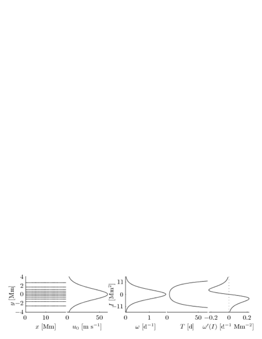
Figure 1: For the streamfunction $\psi_{0}(y)=-U_{0}L\tanh(y/L)$: (a) selected level surfaces of $\psi_{0}$; (b) $u_{0}(y)$; (c) $\omega(I)$; (d) $T(I)$; (e) $\omega^{\prime}(I)$. In this and subsequent figures, d denotes days and distance is measured in Mm; 1 Mm = 1000 km.

Now consider a superposition of the background zonal jet $\psi_{0}(y)$ and one of the two Rossby wave perturbations included in (12). In the reference frame moving at the phase speed of the Rossby wave the flow is steady. The corresponding streamfunction is

$$\psi(x,y)=cy-U_{0}L\tanh\left(\frac{y}{L}\right)+AU_{0}L\,{\rm sech}^{2}\left(\frac{y}{L}\right)\cos(kx)$$ (15)

where the phase speed $c$, wavenumber $k$ and the dimensionless wave amplitude $A$ are written without subscripts. Nondimensionalization ($\psi\rightarrow\psi/(U_{0}L),x\rightarrow kx,y\rightarrow y/L$) reveals that there are two irreducible dimensionless parameters, $A$ and $c/U_{0}$. A bifurcation diagram in $(A,c/U_{0})$ for this system is shown in Fig. 2. This figure shows that there are three regions, corresponding to topologically distinct streamfunction structures, and two critical curves that separate these regions. Level surfaces of $\psi$ in each of the three regions and on the two critical lines are shown in the figure. Holding $A\neq 0$ constant while $c/U_{0}$ is increased reveals all possible streamfunction topologies. For small $c/U_{0}$ the streamfunction is characterized by hyperbolic heteroclinic chains both above and below a spatially periodic eastward jet near $y=0$. As $c/U_{0}$ is increased, a critical value is encountered, at which the two hyperbolic heteroclinic chains merge and the eastward jet disappears. A further increase of $c/U_{0}$ leads to the formation of homoclinic hyperbolic chains above and below a westward jet. As a second critical value of $c/U_{0}$ is passed, the hyperbolic homoclinic chains are destroyed via saddle-node annihilation. For large $c/U_{0}$ the flow is everywhere westward without stagnation points. Similar behavior was noted previously by del-Castillo-Negrete and Morrison (1993) using essentially the same model. The importance of Fig. 2 is that it shows that depending on the choice of $A$ and $c/U_{0}$, the zonal jet may be strong, weak or absent entirely. If $A$ and $c/U_{0}$ correspond to a pair which lies on the critical line at which the two hyperbolic heteroclinic chains merge, the eastward jet disappears and the chain of unstable and stable manifolds near $y=0$ is unstable to an arbitrarily small time-dependent perturbation. For the stratospheric polar vortex the relevant (usually) domain of the $(A,c/U_{0})$ parameter space is small values of both parameters (see, e.g., Bowman, 1996). It should be emphasized, however, that when more than one Rossby wave is superimposed on the background zonal jet, as in (13), the choice of which Rossby wave to absorb into the background is arbitrary. Under such conditions the claim that the background flow topology corresponds to the small $c/U_{0}$ region in Fig. 2 is justified only if this is true for $(A_{i},c_{i}/U_{0})$ for all of the waves present. Although the preceding discussion was motivated by a particular model streamfunction, equation (15), the qualitative features that we have described are expected to be broadly applicable to Rossby wave perturbations to zonal jets.

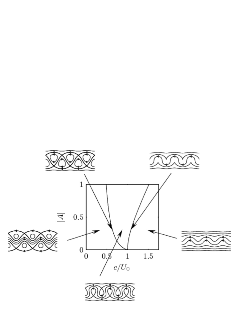
Figure 2: Bifurcation diagram in the $(A,c/U_{0})$ parameter space corresponding to the streamfunction $\psi(x,y)=cy-U_{0}L\tanh(y/L)+AU_{0}L{\rm sech}^{2}(y/L)\cos(kx)$. There are three topologically distinct regions and two critical curves separating these regions. Selected level surfaces of $\psi(x,y)$ in each of the three regions and on the two critical curves are shown. In the level surface plots zonal wavenumber three is assumed so $k=k_{3}$, and $0\leq k_{3}x\leq 6\pi$.

For any steady streamfunction $\psi=\psi(x,y)$ the Lagrangian equations of motion (1) can be transformed to action-angle form. The equations of motion in action-angle form are identical to the equations described above, but the transformation from $\psi(x,y)$ to $\bar{H}(I)$ is more complicated than the trivial relabelling of coordinates described above. More generally, $I(\bar{H})=(2\pi)^{-1}\oint x(y,\bar{H})dy=-(2\pi)^{-1}\oint y(x,\bar{H})dx$ where $\bar{H}=\psi$ and the integral is around a closed loop in $(x,y)$, and $\theta=\partial G/\partial I$ with $G(y,I)=\int_{0}^{y}x(y^{\prime},\bar{H})dy^{\prime}$. (The equivalence of the two forms of $I(\bar{H})$ given above follows from integration by parts. Note also that on a given level surface of $\psi$, $x(y)$ or $y(x)$ may be multi-valued, dictating that some care be exercised when using these equations, and that there is flexibility in choosing the lower limit in the integral defining $G$.) It is often necessary to define action-angle variables in different regions of $(x,y)$ in a piecewise fashion. We emphasize, however, that once this is done the form of the equations of motion in action-angle variables is that given above. It is important to keep in mind that $I$ is simply a label for a particular trajectory or, equivalently, for a particular level surface of $\psi(x,y)$.

For $A=0.3$, $c/U_{0}=0.461$, plots of $|{\bf u}|=(u^{2}+v^{2})^{1/2}$, $\omega(I)$, $T(I)$ and $\omega^{\prime}(I)$ are shown in Fig. 3 for trajectories in the vicinity of the jet core only. Note that, in qualitative agreement with Fig. 1, Fig. 3 shows that in the vicinity of the jet core, $T(I)$ has a local minimum, $\omega(I)$ has a local maximum and $\omega^{\prime}(I)=0$. These features play an important role in the considerations that follow.

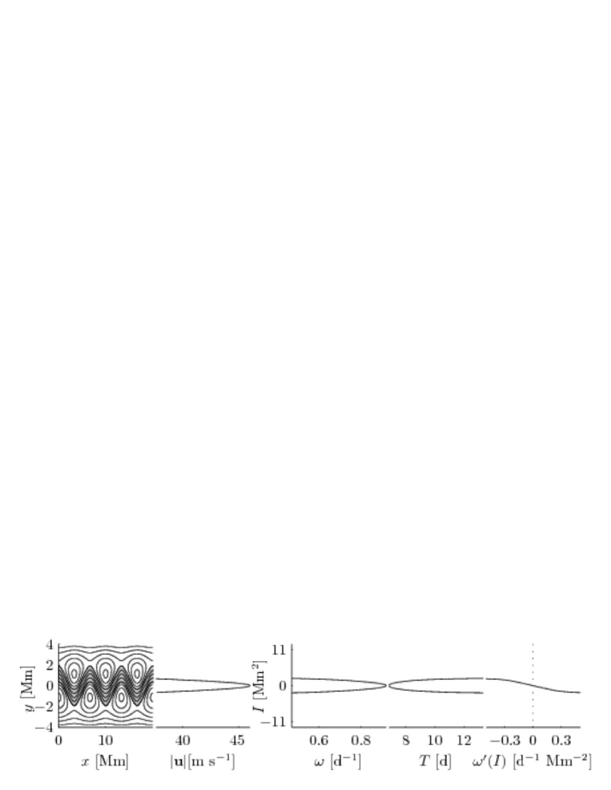
Figure 3: For the streamfunction $\psi(x,y)=c_{3}y-U_{0}L\tanh(y/L)+A_{3}U_{0}L{\rm sech}^{2}(y/L)\cos(k_{3}x)$ with $A_{3}=0.3$, $c_{3}/U_{0}=0.461$: (a) selected level surfaces of $\psi(x,y)$; (b) $|{\bf u}|(y)$ at $k_{3}x=\pi/2$; (c) $\omega(I)$; d) $T(I)$; and (e) $\omega^{\prime}(I)$. In (b), (c), (d) and (e) only values of $y$ and $I$ corresponding to the shaded region near the jet core in (a) are shown.

We turn our attention now to periodically perturbed systems of the form (14), of which (13) is a special case. With $x$ and $y$ bounded, trajectories lie in a 3-dimensional bounded phase space $(x,y,t\bmod 2\pi/\sigma)$. The usual way to view trajectories in such a system is to construct a Poincare section, which is a slice of the 3-d space corresponding to $t\bmod 2\pi/\sigma={\rm constant}$. Three examples, corresponding to the system described by (13) with three choices of the perturbation strength $A_{2}$, are shown in Fig. 4. On these plots regular (nonchaotic) trajectories appear as discretely sampled smooth curves, while chaotic trajectories appear as sets of discrete samples that fill areas. In the $A_{2}=0$ limit all trajectories are nonchaotic; each curve seen in Fig. 4a can be thought of as a 2-d slice of a torus in $(x,y,t\bmod 2\pi/\sigma)$. For small perturbation strength $A_{2}$ some of the unperturbed tori are seen to survive, while other tori break up forming chains of island-like structures that are surrounded by chaotic seas. In general, as the perturbation strength increases more tori are destroyed and the motion becomes increasingly chaotic.

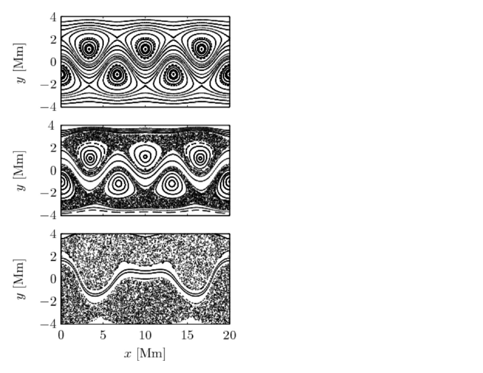
Figure 4: Poincare sections corresponding to the system described by equations (1) and (13) with $A_{3}=0.3$ for three values of $A_{2}$: $0$ (upper plot), $0.1$ (middle plot), and $0.7$ (lower plot). Note the robustness of the tori in the vicinity of the jet core.

Before proceeding, it is instructive to make some seemingly trivial comments about the geometry of systems of the form (14). The tori of the unperturbed system can be thought of as either 1-d surfaces in $(x,y)$ or 2-d surfaces in the 3-d space $(x,y,t\bmod 2\pi/\sigma)$. Because the unperturbed streamfunction does not depend on $\sigma$ the latter view seems like an unnecessary complication, but it turns out to be very useful. The regular trajectories in the perturbed systems shown in Fig. 4 lie on tori (of the second type) of the unperturbed system that survive under perturbation. Because each surviving torus is a 2-d surface in the 3-d space $(x,y,t\bmod 2\pi/\sigma)$, each such torus divides the 3-d space into disjoint ‘inside’ and ‘outside’ regions. A consequence of this is that in the $(x,y)$-plane each surviving torus represents an impenetrable barrier to transport.

The survival of some of the tori of the unperturbed system under small perturbation, as illustrated in Fig. 4, is predicted by the KAM theorem (see, e.g., Arnold et al., 1986; Poschel, 2001). Before giving a more precise statement of the theorem, it is instructive to note that the mechanism that leads to the destruction of the tori of the unperturbed system is excitation of resonances by the time-periodic perturbation. Resonances are excited when the ratio of the frequency of the perturbation $\sigma$ to the frequency of the motion on the unperturbed torus $\omega(I)$ is the ratio of integers. Generically, a continuum of $\omega(I)$ values are present. Under such conditions a fixed $\sigma$ excites infinitely many resonances. In practice, however, the low-order resonances (e.g., $2:1$) are the most important.

With this as a heuristic background, a form of the KAM theorem suitable for systems of the form (14) can now be stated. According to the theorem, tori in the vicinity of those tori in the unperturbed system for which $\omega(I)/\sigma$ is sufficiently irrational survive in the perturbed system provided the strength of the perturbation is sufficiently weak and a nondegeneracy condition, $\omega^{\prime}(I)\neq 0$, is satisfied. The condition that $\omega(I)/\sigma$ is sufficiently irrational is expressed quantitatively by a Diophantine condition; this will not be discussed further as this condition is not central to our arguments.

On the other hand, the nondegeneracy condition plays a critical role in our arguments. In the simplest form of the theorem this condition is $\omega^{\prime}(I)\neq 0$ (or in higher dimensions ${\rm det}(\partial\omega_{i}/\partial I_{j})\neq 0$). This condition guarantees the invertibility of $\omega(I)$, whose importance stems in part from the fact that the theorem guarantees that the torus corresponding to that value of $I$ for which $\omega(I)/\sigma$ is sufficiently irrational survives in the perturbed system. This was the form of the nondegeneracy condition in Kolmogorov’s (1954) original statement of the theorem. Already in his original proof of the theorem, Arnold (1963) noted (in a footnote) that an alternate form of the nondegeneracy condition, the isoenergetic condition, could be used instead. Subsequently, Bruno (1992) and Russmann (1989) announced forms of the theorem that employ less restrictive nondegeneracy conditions.

The Russmann nondegeneracy condition is of particular interest in the present study. The condition is most naturally stated in words: for an autonomous system with $N+1$ degrees of freedom the image of the frequency map $I\rightarrow\omega(I)$ may not lie on any hyperplane of dimension $N$ that passes through the origin. To our knowledge, all published formulations of the KAM theorem to date that make use of the Russmann nondegeneracy condition apply to autonomous systems. To apply such a result to (14) this system must first be written as an equivalent autonomous two degree-of-freedom system with a bounded phase space. The required transformation is a special case of the transformation described at the end of the following section. After performing this transformation, the Russmann condition reduces to a statement that in the 2-d $(\sigma,\omega)$-space, the locus of points $(\sigma,\omega(I))$ must not fall on a line that passes through the origin. This condition is violated only when $\omega(I)=\omega_{o}$, a constant. For our purposes, the significance of the Russmann nondegeneracy condition is that, for systems of the form (14), it is satisfied in a domain that includes an isolated zero of $\omega^{\prime}(I)$. The price paid for making use of the relatively weak Russmann nondegeneracy condition is that a slightly less strong form of the theorem is proved. As noted above, the Kolmogorov condition $\omega^{\prime}(I)\neq 0$ can be used to prove that the torus corresponding to a particular value of $I$ in the unperturbed system survives in the perturbed system. In contrast, when the Russmann form of the theorem is applied in the vicinity of a torus for which $I=I_{0}$ where $\omega^{\prime}(I_{0})=0$ (an isolated zero) the theorem guarantees only that some tori identified by $I$-values near $I_{0}$ will be present in the perturbed system. Thus, when the Russmann form of the theorem is applied it is not appropriate to refer to surviving tori (see, e.g., Sevryuk, 1995, 2006, for a more complete discussion of this issue). For our purposes this distinction is unimportant in that it makes no difference whether the $I=I_{0}$ torus survives under perturbation; it is important to know only that some nearby tori are present in the perturbed system as any such torus provides a barrier to transport.

Because of its generality, we have chosen to emphasize the importance of the Russmann nondegeneracy condition in our discussion of the stability of tori in the vicinity of that for which $\omega^{\prime}(I)=0$. It is worth noting, however, that other arguments have been used to establish essentially the same result for area-preserving mappings (Delshams and de la Llave, 2000; Simó, 1998).

Consider again the Poincare sections shown in Fig. 4. This figure shows that not only do the tori corresponding to trajectories near the jet core (where $\omega^{\prime}(I)=0$) persist in the perturbed system, but these tori appear to be the most resistant to breaking. Numerical simulations based on model systems reveal that, in general, tori near that for which $\omega^{\prime}(I)=0$ tend to be the most resistant to breaking. Interestingly, for the model parameters used to construct Fig. 4, $\sigma/\omega$ at the jet core is approximately $0.95$. The significance of this ratio is its closeness to unity. On two nearby tori, one on each side of the jet core, the strongest possible $(1:1)$ resonance is excited. In spite of this, tori in the vicinity of the jet core are seen to be preserved for moderate perturbation strengths. The reason for the surprising stability of tori near that for which $\omega^{\prime}(I)=0$ will be described below. We emphasize, however, that the stability of tori near that for which $\omega^{\prime}(I)=0$ is not absolute. If, for instance, $\sigma$ happens to be identical to $\omega(I)$ at the jet core where $\omega^{\prime}(I)=0$, thereby exciting a $1:1$ resonance on the jet core, tori near the jet core are not among the last to break up as the perturbation strength increases.

The fact that tori for which $\omega^{\prime}(I)=0$ are strongly resistant to breaking has been noted in the mathematical literature; Gaidashev and Koch (2004) refer to the “remarkable stability” of such tori. Systems which satisfy this condition are generally described as “shearless” or “nontwist” in the mathematical literature, and have been extensively studied in recent years (see, e.g., del-Castillo-Negrete and Morrison, 1993; Morozov, 2002; Dullin and Meiss, 2003).

We turn our attention now to resonance widths as a means to explain the remarkable stability of tori satisfying the nontwist condition. Resonance widths are important because when neighboring resonances overlap, the intervening tori generally break up; the widely used Chirikov definition of chaos is based on overlapping resonances (see, e.g., Chirikov, 1979; Chirikov and Zaslavsky, 1972; Lichtenberg and Lieberman, 1983). Recall that resonances are excited on tori for which $\omega(I)/\sigma$ is rational. Resonance widths are controlled by the degree of rationality of $\omega/\sigma$, the perturbation strength and a simple geometric factor, which we now consider. A simple analysis (see, e.g., Abdullaev, 1993) reveals that resonance widths scale like $\Delta I\sim|\omega^{\prime}(I)|^{-1/2}$, or $\Delta\omega\sim|\omega^{\prime}(I)|^{1/2}$. Because resonances are excited at discrete values of $\omega$, it is the width $\Delta\omega$, rather than $\Delta I$, that is important in determining whether neighboring resonances overlap. Because $\Delta\omega\sim|\omega^{\prime}(I)|^{1/2}$ small values of $\omega^{\prime}(I)$ are generally associated with small resonance widths, and generally more surviving KAM tori. (The resonance width estimates just quoted follow from a simple perturbation analysis. When $\omega^{\prime}(I)=0$ at the resonance, the width of the resonance $\Delta\omega$ depends on $\omega^{\prime\prime}(I)$ at the resonance. The exact form of this expression is not essential to our argument. What is important is the observation that $\Delta\omega$ is small when $\omega^{\prime}$ is small.)

In the vicinity of the jet core a narrow band of $\omega$-values will be present. Resonances will be excited in this band, but only for very special values of $\sigma$ will these be low-order resonances. The associated widths of these resonances are small owing to the smallness of $|\omega^{\prime}(I)|^{1/2}$ in this region. As a result, mostly nonchaotic motion is preserved near the jet core, not because resonances are not excited, but because the corresponding resonance widths are usually so small that neighboring resonances don’t overlap. Excitation of a low-order resonance very close to the jet core can overcome the smallness of $|\omega^{\prime}(I)|^{1/2}$ and change this picture, so the stability of tori near the jet core is not absolute.

In this section we have considered a steady zonal jet on which two travelling Rossby waves are superimposed. Either of the two Rossby waves can be absorbed into a modified steady background flow. We have shown, using well-known results relating to KAM theory, that, provided certain conditions are met, a typically narrow band of nonchaotic trajectories in the vicinity of the jet core, each lying on a KAM invariant torus, persists in the two wave system and provides a barrier to meridional transport. The barrier is linked to the remarkable stability of KAM tori for which $\omega^{\prime}(I)$ has an isolated zero. The conditions that need to be met for such a barrier to be present are: (1) the rest frame phase speeds of both Rossby waves should not be comparable to the wind speed at the jet core; (2) the Rossby wave amplitudes must not be too large; and (3) low order resonances in the immediate vicinity of the jet core in the moving frame must not be excited.

4 A steady background flow subject to a multiperiodic perturbation

In this section we consider streamfunctions of the form

$$\psi(x,y,t)=\psi_{0}(x,y)+\psi_{1}(x,y,\sigma_{1}t,\ldots,\sigma_{N}t)$$ (16)

where $\psi_{1}$ is a multiperiodic function with constituent periods $2\pi/\sigma_{i},i=1,2,\ldots,N$. It should be noted that a steady zonal flow on which a sum of $N+1$ zonally propagating Rossby waves is superimposed has the form (16) when viewed in the reference frame moving at the phase speed of one of the Rossby waves. The $N=1$ problem treated in the previous section is seen to be a special case of the problem treated here. In this section we show that most of the results discussed in the previous section carry over to the larger and more realistic class of problems considered here with only minor modification.

An important observation relating to systems of the form (16) is that one need only consider frequencies that are incommensurable, i.e., have the property that the ratio of all pairs of frequencies is irrational. Consider, for example, a multiperiodic function with periods 4 and 6 days. This function is a simple periodic function with period 12 days. In general, a reduction of the number of frequencies can be achieved whenever two more of the frequencies are commensurable. Thus, without loss of generality, it may be assumed that $\sigma_{1},\sigma_{2},\ldots,\sigma_{N}$ are incommensurable, i.e., that $\psi_{1}$ is a quasiperiodic with $N$ incommensurable frequencies.

Systems of the form (16) have been intensively studied in recent years. A proof of the KAM theorem for such systems has been provided by Jorba and Simó (1996). Several points relating to the Jorba–Simo work are noteworthy. First, the theorem is formulated as a nonautonomous perturbation to an autonomous one degree of freedom system, so the unperturbed Hamiltonian, which must satisfy a nondegeneracy condition, is the system defined by $\psi_{0}(x,y)$ (after transforming to the action-angle representation). Second, the nondegeneracy condition that the unperturbed Hamiltonian is assumed to satisfy is the Kolmogorov condition $\omega^{\prime}(I)\neq 0$. Third, Diophantine conditions must be satisfied by both $\sigma_{i}/\omega$ and $\sigma_{i}/\sigma_{j}$ $(i\neq j)$. The second point is of particular importance in the present study. Loosely speaking, the Jorba–Simo work shows that the principal difference between the periodic perturbation problem and the quasiperiodic perturbation problem is that in the former problem the surviving KAM tori undergo periodic oscillations in $(x,y)$, while in the latter problem the surviving KAM tori undergo quasiperiodic oscillations in $(x,y)$. Jorba and Simo refer to the latter motion as a “quasiperiodic dance.” For our purposes, this distinction is unimportant; in both cases the surviving KAM tori provide a barrier in $(x,y)$ to transport, as we shall describe in more detail later in this section.

All of the mathematical difficulties associated with a quasiperiodic perturbation $\psi_{1}$ are present even for $N=2$. Because, among all $N\geq 2$, the $N=2$ case is the most convenient choice for numerical purposes, it is natural to focus on that choice. With this in mind we have chosen, for numerical purposes, to use the streamfunction

$$\psi(x,y,t)=c_{3}y-U_{0}L\tanh\left(\frac{y}{L}\right)+A_{3}U_{0}L{\rm sech}^{2}\left(\frac{y}{L}\right)\cos(k_{3}x)\\ +A_{2}U_{0}L{\rm sech}^{2}\left(\frac{y}{L}\right)\cos(k_{2}x-\sigma_{2}t)+A_{1}U_{0}L{\rm sech}^{2}\left(\frac{y}{L}\right)\cos(k_{1}x-\sigma_{1}t).$$ (17)

In the $A_{1}=0$ limit this is identical to the streamfunction described by equation (13). Note that physically equation (17) represents a zonal flow corresponding to $\psi(y)=-U_{0}L\tanh(y/L)$ on which three travelling Rossby-like waves are superimposed in a reference frame moving with speed $c_{3}$, the phase speed of the zonal wavenumber three wave. For convenience, we have assumed that the new perturbation term corresponds to zonal wavenumber one, $k_{1}=2\pi/(2\pi r_{e}\cos 60^{\circ})=2/r_{e}$, and has the same ${\rm sech}^{2}(y/L)$ meridional structure as the $k_{2}$ and $k_{3}$ modes. However, unlike the $k_{2}$ and $k_{3}$ modes, which had some dynamical justification, the $k_{1}$ mode is simply an ad-hoc additive perturbation which is included to illustrate some properties of quasiperiodic systems. With this in mind we have chosen $\sigma_{1}/\sigma_{2}$ to be the golden mean $(\sqrt{5}-1)/2$ (whose continued fraction representation identifies it as the most irrational real number).

Numerical simulations based on the system defined by (17) are shown in Figs. 5 and 6. Figure 5 shows the time evolution of two sets of air parcels at times ranging from $t=0$ to $t=81$ days. The initial conditions are chosen to fall on two zonal lines $y={\rm constant}$ on opposite sides of the zonal jet. It is seen that after 81 days each side of the jet is well stirred, as indicated by what appears to be random distributions of dots on each side of the jet, but there is no transport across a wavy boundary near the core of the jet. The cause of this behavior is a thin band of KAM invariant tori near the jet core that survive in the perturbed system and form a meridional transport barrier. This thin band of KAM invariant tori that separate the polar from the midlatitude region in our idealized system undulates in a quasiperiodic fashion in time; this is the “quasiperiodic dance” referred to by Jorba and Simo. Further support for this interpretation of Fig. 5 is provided by the results shown in Fig. 6. In that figure, for the same model system, finite time Lyapunov exponents are shown as a function of initial condition for a set of air parcel trajectories that spans the zonal jet. This figure shows that the region in the immediate vicinity of the jet core is characterized by small Lyapunov exponent estimates. This behavior is consistent with the interpretation that there is a narrow band of surviving tori (on which motion is nonchaotic) in this region.

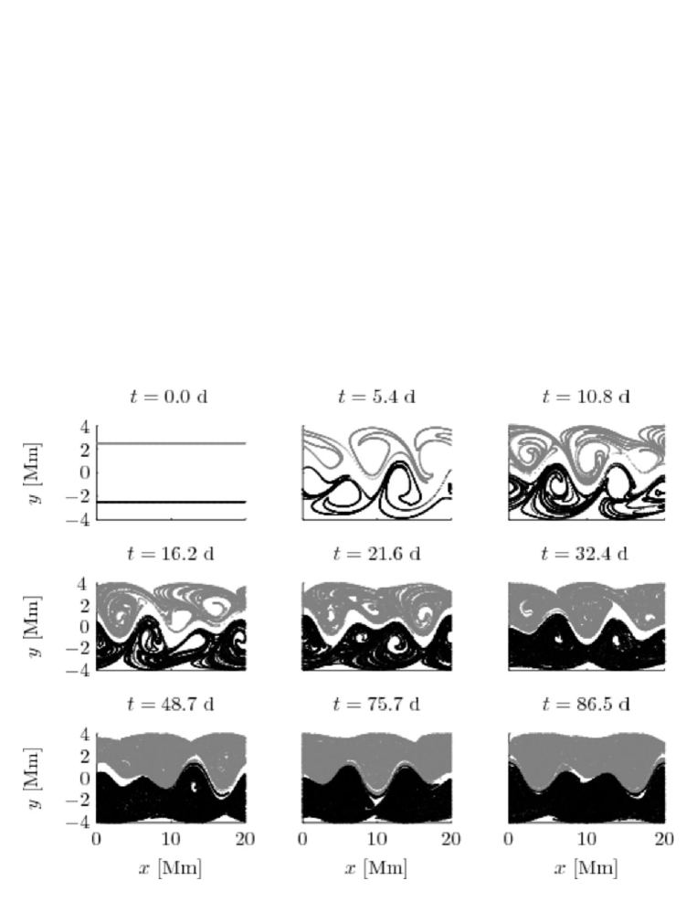
Figure 5: Time evolution of two sets of 25000 points that at $t=0$ fall on zonal lines on opposite sides of the core of the zonal jet in the system described by equations (1) and (17) with $A_{3}=0.3$, $A_{2}=0.4$, $A_{1}=0.075$. Note that, although trajectories are predominantly chaotic, there is no transport across an undulating barrier in the vicinity of the jet core.

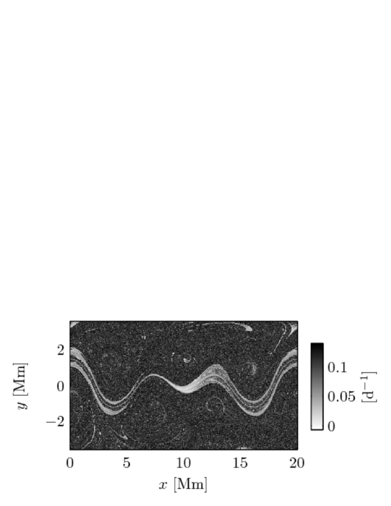
Figure 6: Finite-time Lyapunov exponent estimates as a function of initial position for the system described by equations (1) and (17) with $A_{3}=0.3$, $A_{2}=0.4$, $A_{1}=0.075$. The integration time for the estimates shown is 86.5 days. Note that the region in the vicinity of the jet core is characterized by small Lyapunov exponent estimates.

The qualitative features of Figs. 5 and 6 are consistent with available observational evidence. Consistent with Fig. 5 are satellite-based measurements of ozone distributions in the austral spring; see, e.g., Bowman and Mangus (1993) or the NASA/TOMS web site (http://jwocky.gsfc.nasa.gov/eptoms/ep_v8.html). These observations consistently reveal a sharp boundary between low ozone concentration air inside the stratospheric polar vortex and high ozone concentration air outside the polar vortex. Aircraft-based measurements (see, e.g., Starr and Vedder, 1989) reveal an even sharper boundary between these regions than is suggested by satellite-based measurements; this is not surprising given that the satellite measurements are integral measurements through the entire atmosphere. Our Fig. 6, which indicates that the perimeter of the polar vortex is a narrow nonchaotic barrier that separates two predominantly chaotic regions, is consistent with Fig. 8 in Koh and Legras (2002), Fig. 2 in Pierce and Fairlie (1993) and the observation by Chen (1994) that imbedded in the narrow barrier between the inside and outside of the vortex is a potential vorticity contour that grows at a locally minimal rate.

Figures 5 and 6 suggest that the most robust of the tori of the original system are those in the vicinity of the core of the jet where $\omega^{\prime}(I)=0$. This observation is not surprising as it is consistent with the discussion in the previous section relating to resonance widths. But the observation does serve to identify a weakness in our argument, however, inasmuch as the Jorba–Simo proof of the KAM theorem for quasiperiodic systems makes use of the simplest (Kolmogorov) nondegeneracy condition $\omega^{\prime}(I)\neq 0$. Thus the Jorba–Simo form of the KAM theorem does not address the stability of tori near the jet core, i.e., those that are apparently the most stable. (One might argue that the theorem holds for tori that are arbitrarily close to that for which $\omega^{\prime}(I)=0$, but this is not entirely satisfactory in our view given our focus on the jet core.) What is needed to rigorously complete our argument is a proof of the KAM theorem for quasiperiodic systems (16) that makes use of a Russmann-like nondegeneracy condition rather than the Kolmogorov condition. So far as we are aware, such a proof has not been published to date. Our numerical simulations, including but not limited to Figs. 5 and 6, strongly suggest that the theorem holds for quasiperiodic systems (16) for which the background $\omega^{\prime}(I)$ has an isolated zero.

We turn our attention now to justifying the claim, made above without proof, that for quasiperiodic systems (16) KAM tori provide a barrier to transport. Recall that for periodic systems (14) this property was established by noting that each KAM torus is a 2-dimensional surface in the 3-dimensional space $(x,y,t\bmod 2\pi/\sigma)$ that divides the 3-d space into nonintersecting “inside” and “outside” regions. An extension of the same argument applies to the quasiperiodic problem. To see this, note first that the nonautonomous 1 degree-of-freedom system described by equations (1) and (16) can be written as an equivalent autonomous $N+1$ degree-of-freedom system,

$$\frac{dq_{i}}{d\tau}=\frac{\partial H}{\partial p_{i}},\quad\frac{dp_{i}}{d\tau}=-\frac{\partial H}{\partial q_{i}},\quad i=1,2,\ldots,N+1$$ (18)

where $q_{i}=\sigma_{i}t$, $p_{i}=-\psi/\sigma_{i}$, $i=1,2,\ldots,N$, and $q_{N+1}=y$, $p_{N+1}=x$, with

$$H({\bf p},{\bf q})=\psi(p_{N+1},q_{N+1};q_{1},q_{2},\ldots,q_{N})+\sum_{i=1}^{N}\sigma_{i}p_{i}.$$ (19)

It is straightforward to verify that (18) and (19) reduce to $dt/d\tau=1$, equations (1) and $d\psi/dt=\partial\psi/\partial t$. An important property of the transformed system (18, 19) is that each trajectory is constrained by the presence of $N$ integrals (sometimes called constants of the motion), i.e., $N$ functions $f_{i}({\bf p},{\bf q})$, $i=1,2,\ldots,N$ for which $df_{i}/d\tau=0$. These integrals are $H$ and $f_{i}=q_{i}/\sigma_{i}-q_{N}/\sigma_{N}$, $i=1,2,\ldots,N-1$. If one additional independent integral can be found, the system (18, 19) can be solved by quadratures and is said to be integrable. (This should come as no surprise because the original system (1, 16) also lacks only one integral to render it integrable.) For our purposes, the principal significance of the $N$ integrals is that, because of their presence, each trajectory in the $2(N+1)$-dimensional phase space, lies on a surface of dimension $2(N+1)-N=N+2$. In a near-integrable system of this type in which both KAM tori and chaotic trajectories are present, the tori have dimension equal to the number of degrees of freedom, $N+1$. In the $N+2$-dimensional space that are filled by chaotic trajectories, the $N+1$-dimensional KAM tori serve as impenetrable transport barriers. (The significance of these numbers is that the dimension of the KAM tori is one less than the dimension of the space that the chaotic trajectories fill. Note, for example, that in $(x,y,z)$ the 1-d circle $x^{2}+y^{2}=1,z=0$ divides the 2-d $z=0$ plane into nonintersecting inside and outside regions, but the same 1-d circle does not divide the 3-d $(x,y,z)$ volume into nonintersecting inside and outside regions.)

The argument just given shows that in the system described by (18) and (19) Arnold diffusion does not occur. Loosely speaking, this is the process which allows chaotic trajectories to bypass KAM invariant tori. This process occurs in near-integrable autonomous systems with $N\geq 3$ degrees of freedom which, under perturbation, are constrained by only one integral $H$. For such systems phase space has dimension $2N$, chaotic trajectories lie on surfaces of dimension $2N-1$, while KAM invariant tori have dimension $N$; for $N\geq 3$ these tori do not serve as impenetrable barriers to the chaotic trajectories. The cause of the absence of Arnold diffusion in the system described by (18) and (19) is the integrals in addition to $H$ that constrain the motion of all trajectories.

In this section we have argued that, with some minor modifications, the conclusions of the previous section carry over to a multiperiodic perturbation. Unlike the results of the previous section, however, the multiperiodic argument lacks mathematical rigor in that, to date, no proof of a KAM theorem for quasiperiodically perturbed Russmann-nondegenerate Hamiltonians has been published. Numerical simulations provide strong evidence that such a result holds. With this in mind, we state with some confidence that the qualitative features that were described in the previous section – the robust nature of nonchaotic trajectories near the jet core that serve to isolate chaotic trajectories on opposite sides of the jet – are expected to be seen whether there are 2 or 20 Rossby waves superimposed on the background zonal jet.

5 Summary and discussion

In this paper we have argued, using several nontrivial extensions of the basic KAM theorem, that, under commonly encountered conditions, the zonal jet at the perimeter of the stratospheric polar vortex provides a robust barrier to the meridional transport of passive tracers. In the model employed, the perturbation to the background steady zonal jet was assumed to consist of a sum of travelling Rossby waves. The transport barrier is comprised of a typically narrow band of nonchaotic trajectories, each lying on a KAM invariant torus which is labelled by $I$, that survive in the perturbed system. These tori tend to be the most resistant to break-up under perturbation because they are close to the unperturbed streamline near the jet core for which $\omega^{\prime}(I)=0$ and because resonance widths $\Delta\omega$ are approximately proportional to $|\omega^{\prime}(I)|^{1/2}$. The required extensions to the basic KAM theorem that we have made use of to arrive at this conclusion are: 1) applicability of the theorem to multiperiodic systems, including the absence of Arnold diffusion in such systems; and 2) applicability of the theorem when the usual (Kolmogorov) nondegeneracy condition $\omega^{\prime}(I)=0$ is violated. Our argument falls short of complete mathematical rigor because, to our knowledge, published proofs of the KAM theorem for quasiperiodically perturbed systems make use of the Kolmogorov nondegeneracy condition, rather than the Russmann condition, as required for our purposes. (Note, however, that numerical simulations strongly suggest that the theorem is satisfied for Russmann-nondegenerate streamfunctions subject to quasiperiodic perturbations, indicating that our argument is firmly, if not rigorously, grounded.) Also, it should be emphasized that even rigorous applicability of a form of the theorem to trajectories in the vicinity of the jet core will not guarantee that for all perturbations the corresponding tori will survive and provide a barrier to meridional transport. KAM invariant tori may not survive in the perturbed system for some combination of the following reasons: (1) the phase speed of one of the more energetic Rossby waves is close to the zonal velocity at the jet core; (2) the perturbation excites a low-order resonance on one of the tori in close proximity to that for which $\omega^{\prime}(I)=0$; or (3) the amplitude of the perturbation is too large. In spite of these caveats, our simulations suggest that, under conditions similar to those found in the austral winter and spring, the transport barrier near the core of the zonal jet at the perimeter of the polar vortex is very robust.

Our KAM-theory-based explanation of the mechanism by which the stratospheric polar vortex serves as a barrier to meridional transport of passive tracers (such as ozone-depleted air within the vortex) differs from the potential vorticity barrier argument introduced originally by McIntyre (1989, see also Juckes and McIntyre 1987). According to that argument, on a given isentropic surface potential vorticity (hereafter PV) is nearly constant following individual air parcels and the PV distribution associated with the background zonal jet is characterized by nearly uniform distributions on each side of the jet separated by a region near the core of the jet within which the PV gradient is strong. If the perturbation to the background PV is sufficiently weak that the background meridional PV structure is largely intact in the perturbed system, then PV conservation leads to the expectation that the PV gradient maximum near the jet core should serve to inhibit meridional transport, i.e., that the PV gradient maximum serves as a “PV-barrier.”

The PV-barrier argument has several weaknesses. First, there is no reason to expect that, in general, the vorticity distribution associated with a zonal jet is characterized by a meridional gradient with a prominent maximum near the jet core. The meridional gradient of the background relative vorticity is the second derivative of $u_{0}(y)$. It is easy to construct examples of jet-like zonal velocity profiles whose second derivative does not have a local maximum near the jet core – a quadratic, for example. Second, even when $u_{0}^{\prime\prime}(y)$ does have a peak near the jet core, the PV-barrier argument holds only for a very weak perturbation. Let $U$ and $L$ denote characteristic velocity and length scales with the subscripts $0$ and $1$ used to denote background and perturbation, respectively. The ratio of the magnitude of the relative vorticity of the perturbation to that in the background is $|\zeta_{1}/\zeta_{0}|=O((L_{0}/L_{1})(U_{1}/U_{0}))$. Under typical ozone-trapping conditions in the stratosphere this ratio is not small owing to the fact that $L_{0}/L_{1}$ is greater than unity. Under typical trapping conditions $\zeta_{1}/\zeta_{0}$ is order unity. Under such conditions the relative vorticity structure of the background flow is not expected to strongly constrain the perturbed system. Third, even when the background zonal jet is characterized by a relative vorticity distribution with a maximum meridional gradient near the jet core and the perturbation is very weak, this argument suggests that the transport barrier should be broad, diffuse and stationary (centered at the latitude of the maximum background vorticity gradient), as opposed to being a narrow, wobbly nearly impermeable barrier. Observational evidence supports the latter view. And fourth, the PV-barrier argument provides no insight into why the transport barrier breaks down (as is readily confirmed in simulations) when one of the dominant Rossby wave phase speeds is comparable to the jet core velocity, or when a low order resonance is excited by one of the dominant Rossby waves. In contrast, our KAM-theory-based argument: (1) is robust inasmuch as it requires only that $u_{0}(y)$ has a local maximum, but assumes nothing about $u_{0}^{\prime\prime}(y)$; (2) holds when $|\zeta_{1}/\zeta_{0}|$ is $O(1)$ (the KAM theorem assumes that the perturbation is small but numerical simulations reveal that provided no low-order resonances are excited, KAM tori survive even when $(U_{1}/U_{0})$ is $O(1)$); (3) naturally explains the occurrence of a narrow impermeable barrier that wobbles in the vicinity of the jet core, and the observation that within this narrow region neighboring trajectories diverge from one another only very slowly; and (4) naturally accounts for the breakdown of the barrier when one of the dominant Rossby wave phase speeds is comparable to the jet core velocity, or when a low order resonance is excited by one of the dominant Rossby waves.

The foregoing arguments should not be interpreted as an assertion that the PV-barrier argument is incorrect. Rather, we are arguing that a PV-barrier is not a necessary condition for trapping of air inside the polar vortex, and that a barrier of this type at the perimeter of the polar vortex is probably also not typical. The latter point is supported by the analysis, based on analyzed winds, of Paparella et al. (1997). Figure 2 in that paper shows that the vortex edge is often not associated with a strong meridional PV gradient, but that the vortex edge does appear to be reliably identified as a maximum of kinetic energy. This behavior is in good qualitative agreement with our arguments (recall our Fig. 3) in that in the background environment the trajectory for which $\omega^{\prime}(I)=0$ is close to that for which the kinetic energy is maximum.

The transport barrier at the perimeter of the stratospheric polar vortex that we have identified as being due to a thin band of KAM invariant tori can be described as a Lagrangian coherent structure. The subject of Lagrangian coherent structures has been extensively studied in recent years (see, e.g., Malhotra and Wiggins, 1998; Haller, 2000; Haller and Yuan, 2000; Haller, 2001; Haller and Yuan, 2002; Shadden et al., 2005). In most applications the Lagrangian coherent structures of interest are the stable and/or unstable manifolds of perturbed hyperbolic points. Unlike the KAM tori in our study, which constitute global barriers for transport, such invariant manifolds are barriers for transport only in a local sense and for sufficiently short time. Also, while KAM tori are associated with regular motion, the stable and unstable manifolds are generically associated with chaotic motion in the vicinity of their points of intersections (homoclinic points).

A natural and important extension of the mostly theoretical work reported here is to use analyzed winds (following, e.g., Bowman, 1993, 1996, or Koh and Legras 2002) to more thoroughly test the predictions made here versus those of the PV-barrier paradigm. An empirical study of this type must employ spherical coordinates, i.e., $\psi=\psi(\lambda,\varphi,t)$ on a selected isentropic surface where $\lambda$ and $\varphi$ are longitude and latitude, respectively. Questions that could be addressed with such a model include the following. Is our hypothesized rest frame decomposition of $\psi$, $\psi(\lambda,\varphi,t)=\psi_{0}(\varphi)+\psi_{1}(\lambda,\varphi,t)$ where $\psi_{1}$ is a superposition of zonally propagating Rossby waves, a good approximation? Are vorticity distributions consistent with the PV-barrier paradigm? Is the transport barrier a thin wobbly region on which Lagrangian motion is nonchaotic, as we predict? Is the transport barrier associated with a maximum PV gradient, a maximum of kinetic energy, or something else? Is the breakup of the transport barrier on a given isentropic surface caused by either the phase speed of one of the dominant Rossby waves being comparable to the wind speed at the jet core or the excitation of a low-order resonance, as we have suggested?

This work was supported by the U.S. National Science Foundation, grant CMG0417425.

Figure Captions

Fig. 1. For the streamfunction $\psi_{0}(y)=-U_{0}L\tanh(y/L)$: (a) selected level surfaces of $\psi_{0}$; (b) $u_{0}(y)$; (c) $\omega(I)$; (d) $T(I)$; (e) $\omega^{\prime}(I)$. In this and subsequent figures, d denotes days and distance is measured in Mm; 1 Mm = 1000 km.

Fig. 2. Bifurcation diagram in the $(A,c/U_{0})$ parameter space corresponding to the streamfunction $\psi(x,y)=cy-U_{0}L\tanh(y/L)+AU_{0}L{\rm sech}^{2}(y/L)\cos(kx)$. There are three topologically distinct regions and two critical curves separating these regions. Selected level surfaces of $\psi(x,y)$ in each of the three regions and on the two critical curves are shown. In the level surface plots zonal wavenumber three is assumed so $k=k_{3}$, and $0\leq k_{3}x\leq 6\pi$.

Fig. 3. For the streamfunction $\psi(x,y)=c_{3}y-U_{0}L\tanh(y/L)+A_{3}U_{0}L{\rm sech}^{2}(y/L)\cos(k_{3}x)$ with $A_{3}=0.3$, $c_{3}/U_{0}=0.461$: (a) selected level surfaces of $\psi(x,y)$; (b) $|{\bf u}|(y)$ at $k_{3}x=\pi/2$; (c) $\omega(I)$; (d) $T(I)$; and (e) $\omega^{\prime}(I)$. In (b), (c), (d) and (e) only values of $y$ and $I$ corresponding to the shaded region near the jet core in (a) are shown.

Fig. 4. Poincare sections corresponding to the system described by equations (1) and (13) with $A_{3}=0.3$ for three values of $A_{2}$: $0$ (upper plot), $0.1$ (middle plot), and $0.7$ (lower plot). Note the robustness of the tori in the vicinity of the jet core.

Fig. 5. Time evolution of two sets of 25000 points that at $t=0$ fall on zonal lines on opposite sides of the core of the zonal jet in the system described by equations (1) and (17) with $A_{3}=0.3$, $A_{2}=0.4$, $A_{1}=0.075$. Note that, although trajectories are predominantly chaotic, there is no transport across an undulating barrier in the vicinity of the jet core.

Fig. 6. Finite-time Lyapunov exponent estimates as a function of initial position for the system described by equations (1) and (17) with $A_{3}=0.3$, $A_{2}=0.4$, $A_{1}=0.075$. The integration time for the estimates shown is 86.5 days. Note that the region in the vicinity of the jet core is characterized by small Lyapunov exponent estimates.

References

- Abdullaev (1993) Abdullaev, S. S., 1993: Chaos and the Dynamics of Rays in Waveguide Media. vol. 6, Gordon and Breach.
- Arnold (1963) Arnold, V. I., 1963: Proof of a theorem of A. N. Kolmogorov on the persistence of quasi-periodic motions under small perturbations of the Hamiltonian. Russ. Math. Surveys, 18, 9–36.
- Arnold et al. (1986) Arnold, V. I., V. V. Kozlov, and A. I. Neistadt, 1986: Mathematical Aspects of Classical and Celestial Mechanics. vol. 3 of Encyclopedia of Mathematical Sciencies, Springer.
- Binson and Legras (2002) Binson, J., and B. Legras, 2002: Relation between kinematic boundaries, stirring, and barriers for the Antartic polar vortex. J. Atmos. Sci., 59, 1,198–1,212.
- Bowman (1993) Bowman, K. P., 1993: Large-scale isentropic mixing properties of the antartic polar vortex from analysed winds. J. Geophys. Res., 98, 23,013–23,027.
- Bowman (1996) Bowman, K. P., 1996: Rossby wave phase speeds and mixing barriers in the stratosphere. part I: Observations. J. Atmos. Sci., 53, 905–916.
- Bowman and Mangus (1993) Bowman, K. P., and N. J. Mangus, 1993: Observations of deformation and mixing of the total ozone field in the antartic polar vortex. J. Atmos. Sci., 50, 2915–2921.
- Bruno (1992) Bruno, A. D., 1992: On conditions for nondegeneracy in Kolmogorov’s theorem. Soviet Math. Dokl., 45, 221–225.
- Chen (1994) Chen, P., 1994: The permeability of the antartic vortex edge. J. Geophys. Res., 99, 20,563–20,571.
- Chirikov (1979) Chirikov, B. V., 1979: A universal instability of many-dimensional oscillator systems. Phys. Rep., 52, 265–379.
- Chirikov and Zaslavsky (1972) Chirikov, B. V., and G. M. Zaslavsky, 1972: Stochastic instability of nonlinear oscillations. Sov. Phys. Usp., 14, 549–672.
- Dahlberg and Bowman (1994) Dahlberg, S. P., and K. P. Bowman, 1994: Climatology of large-scale isentropic mixing in the Artic winter stratosphere from analysed winds. J. Geophys. Res., 99, 20,585–20,599.
- del-Castillo-Negrete and Morrison (1993) del-Castillo-Negrete, D., and P. J. Morrison, 1993: Chaotic transport by Rossby waves in shear flow. Phys. Fluids A, 5(4), 948–965.
- Delshams and de la Llave (2000) Delshams, A., and R. de la Llave, 2000: KAM theory and a partial justification of Greene’s criterion for non-twist maps. SIAM J. Math. Anal., 31, 1,235–1,269.
- Dullin and Meiss (2003) Dullin, H. R., and J. D. Meiss, 2003: Twist singularities for symplectic maps. Chaos, 13, 1–16.
- Gaidashev and Koch (2004) Gaidashev, D., and H. Koch, 2004: Renormalization and shearless invariant tori: numerical results. Nonlin., 17, 1713–1722.
- Haller (2000) Haller, G., 2000: Finding finite-time invariant manifolds in two-dimensional velocity fields. Chaos, 10, 99–108.
- Haller (2001) Haller, G., 2001: Lagrangian structures and the rate of starin in a partition of two-dimensional turbulence. Phys. Fluids, 13, 3,365–3,385.
- Haller and Yuan (2000) Haller, G., and G. Yuan, 2000: Lagrangian coherent structures and mixing in two-dimensional turbulence. Physica D, 147, 352–370.
- Haller and Yuan (2002) Haller, G., and G. Yuan, 2002: Lagrangian coherent structures from approximate velocity data. Physics Fluid, 14, 1851–1861.
- Holton et al. (1995) Holton, J. R., P. R. Haynes, M. E. McIntyre, A. R. Douglas, R. B. Rood, and L. Pfister, 1995: Stratosphere-troposphere exchange. Rev. Geophys., 33, 403–439.
- Jorba and Simó (1996) Jorba, Á., and C. Simó, 1996: On quasi-periodic perturbations of elliptic equilibrium points. SIAM J. Math. Anal., 27, 1,704–1,737.
- Juckes and McIntyre (1987) Juckes, N. M., and M. E. McIntyre, 1987: A high-resolution one-layer model of breaking planetary waves in the stratosphere. Nature, 328, 590–596.
- Koh and Legras (2002) Koh, T. Y., and B. Legras, 2002: Hyperbolic lines and the stratospheric polar vortex. Chaos, 12, 328–394.
- Koh and Plumb (2000) Koh, T. Y., and R. A. Plumb, 2000: Lobe dynamics applied to barotropic rossby wave breaking. Physics Fluids, 12, 1518–1528.
- Kolmogorov (1954) Kolmogorov, A. N., 1954: On the persistence of conditionally periodic motions under as small change of the Hamilton function. Dokl. Akad. Nauk SSSR, 98, 525–530. Engl. transl. in G. Casati and J. Ford (eds), Stochastic Behavior in Classical and Quantum Hamiltonian Systems, Lect. Notes Physics 93: 51–56 (1979).
- Kovalyov (2000) Kovalyov, S., 2000: Phase space structure and anomalous diffusion in a rotational fluid experiment. Chaos, 10, 153–165.
- Kuo (1949) Kuo, H., 1949: Dynamic instability of two-dimensional non-divergent flow in a barotropic atmosphere. J. Meteor., 6, 105–122.
- Lefevre et al. (1994) Lefevre, F., G. P. Brasseur, I. Folkins, A. K. Smith, and P. Simon, 1994: Chemestry of the 1991–1992 stratospheric winter – 3-dimensional model simulations. J. Geophys. Res., 99, 8183–8195.
- Lichtenberg and Lieberman (1983) Lichtenberg, A. G., and M. A. Lieberman, 1983: Regular and Stochastic Motion. Springer.
- Lipps (1962) Lipps, F., 1962: The barotropic stability of the mean winds in the atmosphere. J. Fluid Mech., 12, 397–407.
- Malhotra and Wiggins (1998) Malhotra, N., and S. Wiggins, 1998: Geometric structures, lobe dynamics, and Lagrangian transport in flows with aperiodic time-dependence, with applications to Rossby wave flow. J. Nonlinear Sci., 8, 401–456.
- McIntyre (1989) McIntyre, M. E., 1989: On the antartic ozono hole. J. Atmos. Terr. Phys., 51, 29–43.
- Morozov (2002) Morozov, A., 2002: Degenerate resonances in hamiltonian systems with 3/2 degrees of freedom. Chaos, 12, 539–548.
- Ngan and Shepherd (1999a) Ngan, K., and T. G. Shepherd, 1999a: A closer look at chaotic advection in the stratosphere. Part I: Geometric structure. J. Atmos. Sci., 56, 4,134–4,152.
- Ngan and Shepherd (1999b) Ngan, K., and T. G. Shepherd, 1999b: A closer look at chaotic advection in the stratosphere. Part II: Statistical diagnostics. J. Atmos. Sci., 56, 4,153–4,166.
- Paparella et al. (1997) Paparella, F., A. Babiano, C. Basdevant, A. Provenzale, and P. Tanga, 1997: A lagrangian study of the antartic polar vortex. J. Geophys. Res., 102, 6765–6773.
- Pierce and Fairlie (1993) Pierce, R. B., and T. D. Fairlie, 1993: Chaotic advection in the stratosphere: Implications for the dispersal of chemically perturbed air from the polar vortex. J. Geophys. Res., 98, 18,589–18,595.
- Poschel (2001) Poschel, J., 2001: A lecture on the classical KAM theorem. Proc. Symp. Pure Math., 69, 707–732.
- Russmann (1989) Russmann, H., 1989: Non-degeneracy in the perturbation theory of integrable dynamical systems. Number Theory and Dynamical Systems, M. M. Dodson and J. A. G. Vickers, Eds., London Math. Soc. Lect. Notes Series, Cambridge University, pp. 5–18.
- Sevryuk (1995) Sevryuk, M. B., 1995: KAM-stable Hamiltonians. J. Dyn. Cont. Sys., 1, 351–366.
- Sevryuk (2006) Sevryuk, M. B., 2006: Partial preservation of frequencies in KAM theory. Nonlin., 19, 1099–1140.
- Shadden et al. (2005) Shadden, S. C., F. Lekien, and J. E. Marsden, 2005: Definition and porperties of Lagrangian coherent structures from finite-time Lyapunov exponents in two-dimensional aperidic flows. Physica D, 212, 271–304.
- Simó (1998) Simó, C., 1998: Invariant curves of analytic perturbed nontwist area preserving maps. Regul. Chaotic Dyn., 3(3), 180–195.
- Starr and Vedder (1989) Starr, W. L., and J. F. Vedder, 1989: Measurements of ozono in the antartic atmosphere during august and september 1987. J. Geophys. Res., 94, 11,449–11,463.
- Webster et al. (1993) Webster, C. R., et al., 1993: Chlorine chemistry on polar stratospheric cloud particles in the antartic winter. Science, 261, 1130–1134.