Self-similar relaxation dynamics of a fluid wedge in a Hele-Shaw cell

Abstract

Let the interface between two immiscible fluids in a Hele-Shaw cell have, at $t=0$, a wedge shape. As a wedge is scale-free, the fluid relaxation dynamics are self-similar. We find the dynamic exponent of this self-similar flow and show that the interface shape is given by the solution of an unusual inverse problem of potential theory. We solve this problem analytically for an almost flat wedge, and numerically otherwise. The wedge solution is useful for analysis of pinch-off singularities.

Introduction. Interface dynamics between two immiscible fluids in a Hele-Shaw cell have attracted a great interest in the last two decades. Most of the efforts have dealt with forced flows, when a more viscous fluid is displaced by a less viscous fluid. In the forced case the viscous fingering instability ST ; Paterson develops and brings about intricate issues of pattern selection in a channel geometry Kadanoff ; Kessler ; Casademunt , development of fractal structure in a radial geometry Paterson2 , etc. The role of small surface tension in the theory of a forced Hele-Shaw flow is to introduce regularization on small scales. This Letter deals with an unforced Hele-Shaw (UHS) flow Constantin1 ; Almgren ; Sharon ; CLM ; VMS , where surface tension at the fluid interface is the only driving factor. The pertinent free boundary problem here is non-integrable and, because of its non-locality, hard for analysis. To our knowledge, the only known analytical solutions to this class of problems are (i) a linear analysis of the dynamics of a slightly deformed flat or circular interface ST ; Paterson and (ii) a recent asymptotic scaling analysis of the dynamics of a long stripe of an inviscid fluid trapped in a viscous fluid VMS . To get more insight into the physics of UHS flows, we address here the case when one of the fluids at $t=0$ has the form of a wedge. In this case the flow is self-similar. Building on this simplification, we recast the problem into an unusual inverse problem of potential theory. We solve this problem analytically for an almost flat wedge and numerically for several other wedge angles. Finally, we use a wedge solution for analysis of pinch-off events of the UHS flow, which has attracted much interest in theory and experiment Almgren ; Sharon .

Governing equations and self-similarity. Let one of the fluids have a negligible viscosity, so that the pressure inside this fluid is constant and can be taken zero. The velocity of the viscous fluid is $\mathbf{v}\,(\mathbf{r},t)=-(b^{2}/12\mu)\,\nabla p\,(\mathbf{r},t)$, where $p$ is the pressure, $\mu$ is the dynamic viscosity, and $b$ is the plate spacing ST ; Paterson ; Kadanoff . Therefore, the interface speed is

$$v_{n}=-(b^{2}/12\mu)\partial_{n}p\,,$$ (1)

where index $n$ denotes the components of the vectors normal to the interface outwards, and $\partial_{n}p$ is evaluated at the respective points of the interface $\gamma$. As $\mathbf{\nabla}\cdot\mathbf{v}=0$ in the (incompressible) viscous fluid, the pressure there is a harmonic function:

$$\nabla^{2}p=0\,.$$ (2)

The Gibbs-Thomson relation at the interface yields

$$p\,|_{\gamma}=(\pi/4)\,\sigma{\cal K}\,,$$ (3)

where $\sigma$ is surface tension, and ${\cal K}$ is the local curvature of the interface, positive when the inviscid region is convex outwards. As the flow is undriven we demand

$$\partial_{n}p\,=0\;\;\;\mbox{at}\;\;\;\mathbf{r}\to\infty\,.$$ (4)

We assume that the interface has the form of a graph $y=y(x,t)$ and rewrite Eq. (1) as an evolution equation:

$$\partial_{t}y(x,t) = -(b^{2}/12\mu)\,\partial_{n}p\,\sqrt{1+(\partial_{x}y)^{2}}$$ (5)

$$= (b^{2}/12\mu)\left[\partial_{x}y(x,t)\,\partial_{x}p-\partial_{y}p\right]\,,$$

where the derivatives of $p$ are evaluated at the interface.

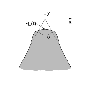
Figure 1: The setting for fluid wedge relaxation.

At $t=0$ the inviscid fluid has the form of a wedge of angle $\alpha$, so that $y=-|x|\cot\,(\alpha/2)$, see Fig. 1. As this initial condition and Eqs. (2)-(5) do not introduce any length scale, the solution must be self-similar B . Let $L(t)$ be the retreat distance of the wedge tip. Then the interface position and the pressure in the viscous fluid can be written as

$$y(x,t) = L(t)\,\Phi\left[\frac{x}{L(t)}\right]\,,$$ (6)

$$p(x,y,t) = \frac{\pi\sigma}{4L(t)}\,P\left[\frac{x}{L(t)},\frac{y}{L(t)}\right]\,,$$ (7)

respectively. We fix the coordinates by choosing $y(x=0,t)=-L(t)$, that is $\Phi(0)=-1$. In the rescaled coordinates $X=x/L(t)$ and $Y=y/L(t)$ the Laplace’s equation (2) keeps its form, while Eq. (3) becomes

$$P\left[X,Y=\Phi(X)\right]=\frac{\Phi^{\prime\prime}(X)}{\left[1+\left[\Phi^{\prime}(X)\right]^{2}\right]^{3/2}}\,,$$ (8)

where primes stand for $X$-derivatives. Now, using Eqs. (6) and (7) in Eq. (5), we arrive at the following equation:

$$\Phi^{\prime}(X)\,\partial_{X}P-\partial_{Y}P=\lambda\left[\Phi(X)-X\Phi^{\prime}(X)\right]\,,$$ (9)

where the derivatives of $P$ are evaluated at the rescaled interface $\Phi(X)$, $L(t)=\left[(\pi\lambda\sigma b^{2}t)/(16\mu)\right]^{1/3}$, and $\lambda$ is an unknown dimensionless parameter. The boundary conditions are $\Phi(0)=-1,\,\Phi^{\prime}(0)=0$ and $\Phi(X\to\pm\infty)=-|X|\cot\,(\alpha/2)$. Note that we have already found the dynamic scaling exponent $1/3$: the same as observed in the relaxation of fractal viscous fingering patterns Sharon ; CLM . The shape function $\Phi(X)$ (and the parameter $\lambda$) for a given wedge angle $\alpha$ is determined by the solution of the following (quite unusual) inverse problem of potential theory. A harmonic function $P(X,Y)$ must obey both a Dirichlet boundary condition [Eq. (8)], and a Neumann boundary condition [Eq. (9)], while the function $\Phi(X)$ must be determined from the demand that these two conditions be consistent. We solved this problem analytically for an almost flat wedge, and numerically otherwise. Before reporting the analytic solution, we present a large-$X$ asymptote of $\Phi(X)$, valid for any wedge angle. It corresponds to the leading term of the multipole expansion of $P(X,Y)$ at large distances. Introduce, for a moment, polar coordinates $r,\phi$ with the origin at the point $X=Y=0$ and measure the polar angle $\phi$ from the ray $Y=-X\cot\,(\alpha/2)$ counterclockwise. At large $|X|$ the curve $Y=\Phi(X)$ is almost flat, so $P[X,\Phi(X)]\to 0$ there by virtue of Eq. (8). Therefore, the leading term of the multipole expansion is $P(r\gg 1,\phi)=\mbox{const}\,r^{-\nu}\sin(\nu\phi)$, where $\nu=(2-\alpha/\pi)^{-1}$ Jackson . Now we employ Eq. (9) and obtain, at $|X|\gg 1$,

$$\Phi(X)=-|X|\cot\,(\alpha/2)+C\,|X|^{-\frac{3\pi-\alpha}{2\pi-\alpha}}+\dots\,,$$ (10)

with an unknown constant $C$ that depends only on $\alpha$.

Almost flat wedge. Let us assume that $\pi-\alpha\ll\pi$, and introduce the small parameter $\varepsilon\equiv\cot(\alpha/2)\ll 1$. We rescale the variables: $X=\xi/\varepsilon$, $Y=\eta/\varepsilon$, $P(X,Y)=\varepsilon^{2}\,U(\xi,\eta)$ and $\lambda=\Lambda\varepsilon^{3}$. In the rescaled varaibles the interface equation is $\eta=\varepsilon\psi(\xi)$, where $\psi(\xi)\equiv\Phi(\xi/\varepsilon)$. Keeping only leading terms, we can rewrite the boundary conditions (8) and (9) for the harmonic function $U(\xi,\eta)$ in the following form:

$$U\left[\xi,\varepsilon\psi(\xi)\right] = \psi^{\prime\prime}(\xi)\,,$$ (11)

$$\partial_{\eta}U\left[\xi,\varepsilon\psi(\xi)\right] = \Lambda\left[\xi\psi^{\prime}(\xi)-\psi(\xi)\right]\,,$$ (12)

where

$$\psi(0)=-1,\,\psi^{\prime}(0)=0,\,\psi(\xi\to\pm\infty)=-|\xi|+o(1)\,.$$ (13)

The rescaled problem does not include $\varepsilon$, except in the second argument of the functions on the left hand side of Eqs. (11) and (12). In view of the condition $\psi(\xi\to\pm\infty)=-|\xi|$ one cannot put the second argument to zero at sufficiently large $|\xi|$. As will be shown below, these values of $\xi$ are exponentially large in $\varepsilon^{-1}$, while at shorter distances one can safely put the second argument to zero.

The problem obtained in this way is soluble exactly. Assume $\psi(\xi)$ is known. Then one can easily find the harmonic function in the upper half-plane $\eta>0$, that satisfies the Dirichlet condition $u(\xi,0)=\psi^{\prime\prime}(\xi)$ on the $\xi$-axis:

$$U(\xi,\eta)=\frac{1}{\pi}\int_{-\infty}^{\infty}\frac{\eta\,\psi^{\prime\prime}(s)\,ds}{(\xi-s)^{2}+\eta^{2}}\,.$$ (14)

Now we should impose the Neumann condition (12) (where we put $\varepsilon=0$). To avoid calculation of hyper-singular integrals, we find the harmonic conjugate

$$V(\xi,\eta)=\frac{1}{\pi}\int_{-\infty}^{\infty}\frac{(\xi-s)\psi^{\prime\prime}(s)\,ds}{(\xi-s)^{2}+\eta^{2}}$$ (15)

and, by virtue of the Cauchy-Riemann conditions, replace $\partial_{\eta}U(\xi,0)$ by $-\partial_{\xi}V(\xi,0)$. This yields a non-standard integro-differential equation

$$\Lambda\left[\xi\psi^{\prime}(\xi)-\psi(\xi)\right]=-\frac{1}{\pi}\frac{d}{d\xi}\,\mathchoice{{\vbox{\hbox{$\textstyle-$}}\kern-4.86108pt}}{{\vbox{\hbox{$\scriptstyle-$}}\kern-3.25pt}}{{\vbox{\hbox{$\scriptscriptstyle-$}}\kern-2.29166pt}}{{\vbox{\hbox{$\scriptscriptstyle-$}}\kern-1.875pt}}\!\int_{-\infty}^{\infty}\frac{\psi^{\prime\prime}(s)\,ds}{\xi-s}\,,$$ (16)

where $\mathchoice{{\vbox{\hbox{$\textstyle-$}}\kern-4.86108pt}}{{\vbox{\hbox{$\scriptstyle-$}}\kern-3.25pt}}{{\vbox{\hbox{$\scriptscriptstyle-$}}\kern-2.29166pt}}{{\vbox{\hbox{$\scriptscriptstyle-$}}\kern-1.875pt}}\!\int$ denotes the principal value of the integral. Fortunately, upon differentiation with respect to $\xi$ Eq. (16) becomes an equation for $\psi^{\prime\prime}(\xi)$ which is soluble by Fourier transform. The result is

$$\psi^{\prime\prime}(\xi)=-\frac{1}{\pi}\int_{-\infty}^{\infty}e^{-\frac{|k|^{3}}{3\Lambda}}\,\cos k\xi\,dk$$ (17)

(the constant of integration is determined from the condition $\int^{\infty}_{-\infty}\psi^{\prime\prime}(\xi)d\xi=-2$). Integrating twice in $\xi$ and using the first two conditions in Eq. (13) yields

$$\psi(\xi)=-1-\frac{2}{\pi}\int_{-\infty}^{\infty}e^{-\frac{|k|^{3}}{3\Lambda}}\,\,\frac{\sin^{2}\frac{k\xi}{2}}{k^{2}}\,dk\,.$$ (18)

To determine $\Lambda$, we expand this expression at $|\xi|\gg 1$:

$$\psi(\xi)=-|\xi|+\frac{2\,\Gamma(2/3)}{\pi(3\Lambda)^{1/3}}-1+\frac{2}{3\pi\Lambda}\,\xi^{-2}+\dots\,,$$ (19)

where $\Gamma(w)$ is the gamma-function singularity . To eliminate the offset ${\cal O}(1)$ we put $\Lambda=(8/3)\,\pi^{-3}[\Gamma(2/3)]^{3}=0.213545\dots$. Though the integrals in Eqs. (17) and (18) can be expressed via the generalized hypergeometric function ${}_{p}F_{q}(a;b;z)$, it is more convenient to keep the integral form small . To complete the solution, we find the rescaled pressure:

$$U(\xi,\eta)=-\frac{1}{\pi}\int_{-\infty}^{\infty}e^{-\frac{|k|^{3}}{3\Lambda}-|k|\eta}\cos k\xi\,\,dk\,.$$ (20)

Now we find the distance $|\xi|=l(\varepsilon)\gg 1$ at which the solution (18) becomes inaccurate, and improve the large-$|\xi|$ asymptote. Let us compare Eq. (19), which becomes

$$\psi(\xi)=-|\xi|+\frac{\pi^{2}}{4[\Gamma(2/3)]^{3}}\,\xi^{-2}\,,\;\;1\ll|\xi|\ll l(\varepsilon)\,,$$ (21)

with the large-$|\xi|$ multipole asymptote (10):

$$\psi(\xi)=-|\xi|+C(\varepsilon)\,|\xi/\varepsilon|^{-\frac{3\pi-\alpha}{2\pi-\alpha}}\,,\,\;\;|\xi|\gg 1\,.$$ (22)

where, for small $\varepsilon$, $-(3\pi-\alpha)/(2\pi-\alpha)\simeq-2+2\varepsilon/\pi\,.$ We see that the last term in Eq. (21) lacks the small correction $2\varepsilon/\pi$ in the exponent of $\xi$. We can match the two asymptotes (21) and (22) in their common region of validity $1\ll|\xi|\ll l(\varepsilon)$. We define $l(\varepsilon)$ as the value of $|\xi|$ for which the correction to the exponent yields a factor $e$: $l(\varepsilon)=e^{\pi/(2\varepsilon)}$ [notice that, at $|\xi|\sim l(\varepsilon)$, the deviation of $\psi(\xi)$ from its flat asymptote $-|\xi|$ is already exponentially small: $\sim e^{-\pi/\varepsilon}$]. The matching yields $C(\varepsilon)$, and we arrive at the improved small-$\varepsilon$ large-$|\xi|$ asymptote:

$$\psi(\xi)=-|\xi|+\frac{\pi^{2}}{4[\Gamma(2/3)]^{3}}\,e^{-\frac{2\varepsilon}{\pi}\ln\varepsilon}\,\xi^{-2+\frac{2\varepsilon}{\pi}}\,.$$ (23)

So far we have dealt with inviscid fluid wedges: $\alpha<180^{\circ}$. Our results, however, can be immediately extended to viscous fluid wedges: $\alpha>180^{\circ}$.

Numerical algorithm and parameters. For a general wedge angle the shape function of the self-similar interface can be found numerically. Instead of dealing with the similarity formulation of the problem (8)-(9), we computed the time-dependent relaxation of wedges of different angles, as described by (rescaled) Eqs. (1)-(4) units . Our numerical algorithm VM employs a variant of the boundary integral method for an exterior Dirichlet problem for a singly connected domain, and explicit tracking of the contour nodes. The harmonic potential is represented as a superposition of potentials created by a dipole distribution with an unknown density $\mathbf{D}$ on the contour. $\mathbf{D}$ is computed from a linear integral equation Tikhonov . Computing another integral of this dipole density yields the harmonic conjugate, whose derivative along the contour is equal to the normal velocity of the interface.

We chose the singly connected domain to be (i) a rhombus with angles $120^{\circ}$ and $60^{\circ}$, (ii) a square, and (iii) a straight cross with aspect ratio $10^{3}$ units . In this manner we could exploit the 4-fold symmetry of the domains and measure the retreat distance of the respective vertexes, $L(t)$, and the rescaled interface shapes $\Phi(X)$ for four wedge angles: $120^{\circ}$, $90^{\circ}$, $60^{\circ}$ and $270^{\circ}$, the latter one corresponding to a $90^{\circ}$ wedge of the viscous fluid. The ultimate shapes of the rhombus- and square-shaped domains are perfect circles. Therefore, to observe the self-similar asymptotics we did the measurements at times much shorter than the characteristic time of relaxation toward a circle, and at distances much smaller than the domain size (so that the effect of the other vertexes could be neglected). For the rhombus and square an equidistant grid with 901 nodes per side was employed. For the quarter of the cross we used 2801 nodes. The time step was taken to be $10^{-3}$ times the maximum of the ratio of the interface curvature radius and the interface speed at the same node. The domain area conservation was used for accuracy control. For the measurements reported here the area was conserved with an accuracy better than $10^{-3}\%$.

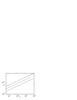
Figure 2: The retreat distance $L(t)$ and its power-law fit for $\alpha=120^{\circ}$ (triangles), $90^{\circ}$ (squares) and $60^{\circ}$ (circles).

Numerical results. We first report the results for the three viscous fluid wedges. Figure 2 shows the retreat distance $L(t)$ for the angles $120^{\circ}$, $90^{\circ}$, and $60^{\circ}$. Power law fits yield $L(t)=0.48\,t^{0.33}$, $0.84\,t^{0.33}$, and $1.33\,t^{0.33}$, respectively, so the dynamic exponent $1/3$ is clearly observed. In the rescaled units, used in the simulations units , the analytical prediction for an almost flat wedge is $L(t)=at^{1/3}$, where $a=(3\Lambda)^{1/3}\varepsilon\simeq 0.862\,\varepsilon$. For $\alpha=120^{\circ}$ and $90^{\circ}$ this yields $a\simeq 0.498$ and $a=0.862$, respectively, in very good agreement with the measured values $0.48$ and $0.84$. Even for $\alpha=60^{\circ}$ the analytical prediction, $a=1.493$, is only $12\%$ higher than the measured value $1.33$.

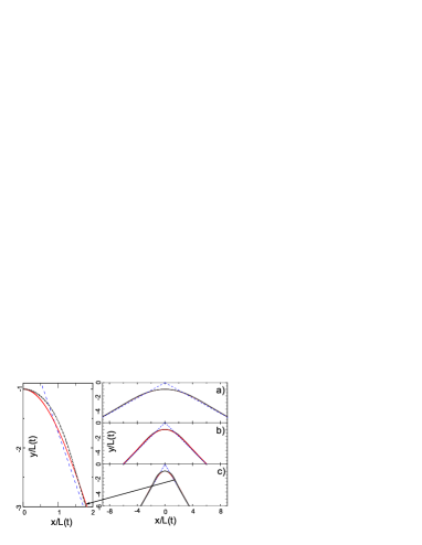
Figure 3: (color online). Right panel: the shape function $\Phi$ for wedges of inviscid fluid: $\alpha=120^{\circ}$ (a), $90^{\circ}$ (b) and $60^{\circ}$ (c). Data for three different times ($2.3\times 10^{-7}$, $1.3\times 10^{-5}$ and $1.1\times 10^{-4}$ for a and c, and $8.2\times 10^{-7}$, $8.9\times 10^{-6}$ and $3.5\times 10^{-5}$ for b) collapse into a single curve. The red solid line is the prediction of the almost-flat-wedge theory, the blue dashed line is the asymptote $Y=-|X|\,\cot{\alpha/2}$. Left panel: a blowup of a part of figure c.

The rescaled shapes of the three evolving wedges are depicted in Fig. 3. That the curves, measured at three different times, collapse into a single curve proves self-similarity. The prediction of our almost-flat-wedge theory, shown on the same three graphs, works very well for $\alpha=120^{\circ}$ and $90^{\circ}$, and fairly well even for $60^{\circ}$.

We also measured, for each of the three values of the wedge angle, the tail of the shape function (the difference between $\Phi(X)$ and $Y=-|X|\,\cot{\alpha/2}$). The results are in excellent agreement with the theoretical prediction, given by the last term in Eq. (10).

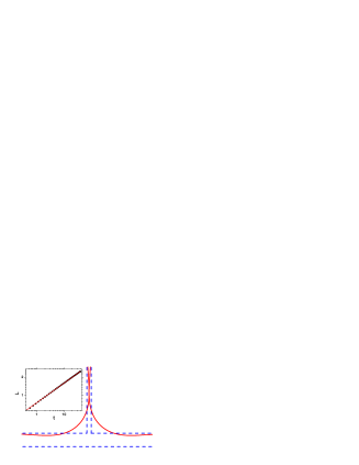
Figure 4: (color online). Pinch-off of a straight branch of thickness $\Delta$ of inviscid fluid. Each of the two viscous fluid wedges corresponds to $\beta=90^{\circ}$ (i.e. $\alpha=270^{\circ}$). The blue dashed lines: the interface shape at $t=0$; the red solid lines: the interface shape at the pinch-off time $t=50.65$ (in the units of units ). The inset: the measured viscous fluid retreat distance versus time and its power-law fit $0.74\times t^{0.33}$.

Pinch-offs. The self-similar wedge solutions are useful for analysis of pinch-offs in UHS flows Almgren ; Sharon . Let the inviscid fluid domain represent, at $t=0$, an infinitely long straight branch, coming at an angle $\beta$ from an infinitely long straight “trunk”. The simple physics in the inviscid fluid branch precludes interaction between the two viscous fluid wedges of angles $\beta$ and $\pi-\beta$, which evolve in a self-similar manner, causing the inviscid branch to thin, and ultimately to pinch-off. The $t^{1/3}$ law intrinsic in the self-similar solution implies that the pinch-off time is proportional to the branch thickness cubed. The interface shape at all times prior to the pinch-off can be obtained, with a proper rescaling, from the respective self-similar shape functions of the two viscous fluid wedges. The case of $\beta=90^{\circ}$ is shown in Fig. 4, where the retreat distance, the shape function and the pinch-off time are taken from the previously described simulation of the cross-shaped domain with aspect ratio $10^{3}$.

Summary. We have studied analytically and numerically the surface tension driven flow of a fluid wedge in a Hele-Shaw cell. We have shown that the fluid interface evolves self-similarly, found the asymptotic interface shape at large distances, and recast the problem into an unusual inverse problem of potential theory. We solved this inverse problem analytically in the limit of nearly flat wedge, and performed numerical simulation which support and extend the analytic calculations. Like in the case of self-similar solutions, obtained for wedge-like initial conditions in other surface tension driven flows others , this solution provides a sharp characterization of the UHS flow. It also sheds a new light on the pinch-off singularities of this flow.

References

- (1) P.G. Saffman and G.I. Taylor, Proc. R. Soc. London, Ser. A 245, 312 (1958).
- (2) L. Paterson, J. Fluid Mech. 113, 513 (1981).
- (3) D. Bensimon, L.P. Kadanoff, S. Liang, B.I. Shraiman, and C. Tang, Rev. Mod. Phys. 58, 977 (1986).
- (4) D.A. Kessler, J. Koplik, and H. Levine, Adv. Physics 37, 255 (1988).
- (5) J. Casademunt and F.X. Magdaleno, Phys. Rep. 337, 1 (2000).
- (6) L. Paterson, Phys. Rev. Lett. 52, 1621 (1984), and numerous subsequent works.
- (7) P. Constantin and M. Pugh, Nonlinearity 6, 393 (1993).
- (8) R. Almgren, Phys. Fluids 8, 344 (1996), and references therein.
- (9) E. Sharon, M.G. Moore, W.D. McCormick, and H.L. Swinney, Phys. Rev. Lett. 91, 205504 (2003).
- (10) M. Conti, A. Lipshtat, and B. Meerson, Phys. Rev. E 69, 031406 (2004).
- (11) A. Vilenkin, B. Meerson, and P.V. Sasorov, Phys. Rev. Lett. 96, 044504 (2006).
- (12) G.I. Barenblatt, Scaling, Self-similarity, and Intermediate Asymptotics (Cambridge University Press, Cambridge, 1996).
- (13) J.D. Jackson, Classical Electrodynamics (Wiley, New York, 1975), p. 76.
- (14) The term in Eq. (19) results from the non-analiticity of the function at .
- (15) At small Eq. (18) yields
- (16) In the numerical simulations we measured the distances in units of (the side of the rhombus or square, the thickness of the cross arm), the time in units of , and the viscous fluid pressure in units of . Then Eqs. (1) and (3) become and , so the rescaled problem is parameter-free.
- (17) A. Vilenkin and B. Meerson, arXiv physics/0512043.
- (18) A.N. Tikhonov and A.A. Samarskii, Equations of Mathematical Physics (Dover, New York, 1990).
- (19) H. Wong, M.J. Miksis, P.W. Voorhees, and S.H. Davis, Acta Mater. 45, 2477 (1997); M.J. Miksis and J.-M. Vanden-Broeck, Phys. Fluids 11, 3227 (1999), and references therein.