Complexities of social networks: A Physicist’s perspective

Preprint no:CU-Physics 02-2006

I Introduction

A large number of natural phenomena in the universe go on oblivious of the presence of any living being, let alone a society. Fundamental science subjects like physics and chemistry deal with laws which would remain unaltered in the absence of life. In biological science, which deals with living beings, the idea of a society may exist in a basic form, e.g., as food chains, struggle for existence etc., among different species whereas present day human society has many more layers as factors like politics, economics or psychology dictate its evolution to a large extent.

A society of human beings can be conceived in different ways as it involves different kinds of contacts. Based on a certain kind of interaction, a collection of human beings may be thought of as a network where the individuals are the nodes and the links are formed whenever two of them interact in the defined way [1]. An interesting aspect of several such social networks is that these show small world effect, a phenomenon which has been shown to exist in diverse kinds of networks [2]. Small world effect and other interesting features shared by real world networks of different nature have triggered off a tremendous activity of research among scientists of different disciplines [3, 4, 5]. Physicists’ interests in networks lie in the fact that these show interesting phase transitions as far as equilibrium and dynamic properties are concerned. The tools of statistical physics come handy in the analytical and numerical studies of networks. Also, physics of systems embedded in small world networks raise interesting questions.

In this article we discuss the properties of social networks which have received much attention during recent years. The topic of social networks is vast and covers many aspects. Obviously, all the issues are too difficult to address in a single review and thus we have tried to give an overview of the subject, emphasising a physicist’s perspective whenever possible.

II The beginning: Milgram’s experiments

The first real world network which showed the small world effect was a social network. This was the result of some experimental studies by the social psychologist, Milgram [6]. In Milgram’s experiments, various recruits in remote places of Kansas and Nebraska were asked to forward letters to specific addresses in Cambridge and Boston in Massachusetts. A letter had to be hand-delivered only through persons known on first-name basis. Surprisingly, it was found that on an average six people were required for a successful delivery. The number 6 is approximately $\log(N)$, where $N$ is the total number of people in the USA. In this particular experiment, if a person A gave the letter to B, A and B are said to have a link between them. If B next hands over the mail to C, the effective “distance” between A and C is 2; while between A and B, as well as between B and C, it is 1. Defining distance in this way, Milgram’s experiments show that two persons in a society are separated by an average distance of six steps. This property of having a small average distance in the society is what is known as the small world effect.

It took around thirty years to realise that this small world effect is not unique to the human society but rather possessed by a variety of other real (both natural and artificial) networks. These networks include social networks, Internet and WWW network, power grid network, biological networks, transport networks etc.

III Topological properties of networks

Before analysing a society from the network point of view, it will be useful to summarise the topological properties characterising common small world networks.

A network is nothing but a graph having nodes as the vertices and links between nodes as edges. A typical network is shown in Fig. 1 where there are ten nodes and ten links.

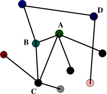
FIG. 1.: A typical network. The shortest distance from A to C is 1 while that from A to D is 3. A,B,C form a cluster.

The shortest distance $S$ between any two nodes A and B is the number of edges on the shortest path from A to B through connected nodes. In Fig. 1, the shortest path from A to D goes through three edges and $S_{AD}=3$. The diameter $D$ of a network is the largest of the shortest distances $S$ and in a small world network (SWN), both the average shortest distance $\langle S\rangle$ and $D$ scale in the same way with $N$, the number of nodes in the network.

Erdös and Rényi studied the random graph [7] in which any two vertices have a finite probability to get linked. In this network or graph, both $D$ and $\langle S\rangle$ were found to vary as $\log(N)$. (This result is true when a minimum number of edges is present in the graph so that a giant structure is formed; if in the graph with $N$ nodes, the connectivity probability of any two nodes is $p$, a giant structure is formed for $pN>1$.)

The network of human population, or for that matter, many other networks can hardly be imagined to be a random network, although the latter has the property of a small average shortest distance between nodes. The other factor which is bound to be present in a social network (like the one considered by Milgram) is the clustering tendency. This precisely means that if A is linked to both B and C there is a strong likelihood that C is also linked to B. This property is not expected to be present in a random network.

Let $a_{ij}$ define the adjacency matrix of the network; $a_{ij}=1$ if nodes $i$ and $j$ are connected and zero otherwise. Then one can quantify the clustering coefficient $C_{i}$ of node $i$ as

$$C_{i}=\Sigma_{j_{1}\neq j_{2}}\frac{2}{k_{i}(k_{i}+1)}{a_{j_{1}j_{2}}},$$ (1)

where $j_{1},j_{2}$ are nodes connected to $i$ and $k_{i}=\Sigma_{j}a_{ij}$, the total number of links possessed by node $i$, also known as its degree (for example in Fig. 1, the degree of node A is 4). Measuring the average clustering coefficient $C=\frac{1}{N}\Sigma_{i}C_{i}$ in several networks, it was observed that the clustering coefficient was order of magnitude higher than that of a random network with the same number of vertices and edges. Thus it was concluded that the real-world networks were quite different from a random network as far as clustering property is concerned. Networks with a small value of $\langle S\rangle$ or $D$ ($O(\log(N))$) together with a clustering coefficient much larger than the corresponding random network were given the name small world network. Mathematically it is possible to distinguish between a small world network and a random network by comparing their clustering coefficients.

Another type of network may be conceived in which the clustering property is high but the average shortest distance between nodes is comparable to $N$. Such networks are called regular networks and thus the small world networks lie in between regular and random networks.

One can find out the probability distribution of the number of neighbours of a node, commonly called the degree, of a network. An interesting feature revealed in many real world networks is the scale-free property [8]. This means that the degree distribution $P(k)$ (i.e., the probability that a node has degree $k$) shows the behaviour $P(k)\sim k^{-\gamma}$, implying the presence of a few nodes which are very highly connected. These highly connected nodes are called the hubs of the network.

It may be mentioned here that in the random graph, $P(k)$ has a different behaviour,

$$P(k)=e^{-\langle k\rangle}\frac{{\langle k\rangle}^{k}}{k!},$$ (2)

where $\langle k\rangle$ is the average degree of the network. $P(k)$ therefore follows a Poisson distribution here decaying rapidly with $k$.

The above features constitute the main properties of networks. Apart from these, many other characteristics have been detected and analysed as research in small world networks increased by leaps and bounds. Some of these, e.g., closeness centrality or betweenness centrality were already quite familiar to social scientists [1].
Closeness centrality: The measure of the average shortest distance of a node to the other nodes in a network is its closeness centrality.
Betweenness centrality: The fraction of shortest paths passing through a node is its betweenness [9, 10]. The more is the betweenness of a node, the more important it is in the network since its absence will affect the small world property to a great extent. It is not necessarily true that nodes with maximum degree will have the largest closeness or betweenness centrality.
Remaining degree distribution: If we arrive at a vertex following a random edge, the probability that it has degree $k$ is $kP(k)$. The remaining degree distribution $q_{k}$, which is the probability that the node has $k$ other edges, is given by

$$q_{k}=\frac{(k+1)P({k+1})}{\Sigma_{j}jP(j)}.$$ (3)

Assortativity : This measure is for the correlation between degrees of nodes which share a common edge. A straightforward measure will be to calculate the average degree $\langle k_{nn}\rangle$ of the neighbours of a vertex with degree $k$. If $\frac{d\langle k_{nn}\rangle}{dk}>0$, it will mean a positive correlation or assortativity in the network. A negative value of the derivative denotes disassortativity and a zero value would mean no correlation. A more rigorous method of calculating the assortativity is given in [11], where one defines a quantity $r$ as

$$r=\frac{M^{-1}\Sigma_{i}j_{i}k_{i}-[M^{-1}\Sigma_{i}\frac{1}{2}(j_{i}+k_{i})]^{2}}{M^{-1}\Sigma_{i}\frac{1}{2}(j_{i}^{2}+k_{i}^{2})-[M^{-1}\Sigma_{i}\frac{1}{2}(j_{i}+k_{i})]^{2}},$$ (4)

where $j_{i}$ and $k_{i}$ are the degrees of the vertices connected by the $i$th edge ($i=1,2,....,M$) and $M$ is the total number of edges in the network. Again, high assortativity means that two nodes which are both highly connected tend to be linked and $r>0$. A negative value of $r$ implies that nodes with dissimilar degrees are more likely to get connected. A zero value implies no correlation of node degrees and their connectivity.

Community structure: This is a property which is highly important for the social networks. More often than not we find a society divided into a number of communities, e.g, based on profession, hobby, religion etc. For the scientific collaboration network, communities may be formed with scientists belonging to different fields of research, for example, physicists, mathematicians or biologists. Within a community also, there may be different divisions like physicists may be classified into different groups, e.g., high energy physicists, condensed matter physicists and so on.

It is clear that the properties of a network simply depends on the way the links are distributed among the vertices, or to be precise, on the adjacency matrix. Till now we have not specified anything about the links. Links in the networks may be both directed and undirected, e.g., in a e-mail network [12], if A sends a mail to B, we have a directed link from A to B. Edges may also be weighted; weights may be defined in several ways depending on the type of network. In the weighted collaboration network, two authors sharing a large number of publication have a link which has more weight than that between two authors who have collaborated fewer times.

IV Some prototypes of small world networks

At this juncture, it is useful to describe a few important prototype small world network models which have been considered to mimic the properties of real networks.

A Watts and Strogatz (WS) network

This was the first network model which was successful in reproducing the features of small diameter and large clustering coefficient of a network. The small world effect in networks of varied nature indicated a similarity in the underlying structure of the networks. Watts and Strogtaz [2] conjectured that the geometry of the networks have some common features responsible for the small world effect. In their model, the nodes are placed on a ring. Each node has connection to $k$ number of nearest neighbours initially. With probability $p$, a link is then rewired to form a random long ranged link.

At $p=0$, the shortest paths scale as $N$ and the clustering coefficient of the network is quite high as it behaves as a regular network with a considerable number of nearest neighbours. The remarkable result was, even with $p\to 0$, the diameter of the network is small ($O(\log(N))$). The clustering coefficient on the other hand remains high even when $p\neq 0$ unless $p$ approaches unity. Thus for $p\to 0$, the network has a small diameter as well as high clustering coefficient, i.e., it is a small world network. For $p\to 1$, the network ceases to have a large clustering coefficient and behaves as a random network. This model thus displays phase transitions from a regular to a small world to a random graph by varying a single parameter $p$. Later it was shown to have mean field behaviour in the small world phase [13].

The degree distribution $P(k)$ in this network, however, did not have a power law behaviour but showed an exponential decay with a peak at $\langle k\rangle$.

B Networks with small world and scale-free property

Although the WS model was successful in showing the small world effect, it did not have a power law degree distribution. The discovery of scale-free property in many real world networks required the construction of a model which would have small world as well as scale-free property.

Barabási and Albert (BA) [8] proposed an evolving model in which one starts with a few nodes linked with each other. Nodes are then added one by one. An incoming node will have a probability $\Pi_{i}$ to get attached to the $i$th node already existing in the network according to the rule of preferential attachment which means that

$$\Pi_{i}=k_{i}/\Sigma k_{i},$$ (5)

where $k_{i}$ is the degree of the $i$th node. This implies that a node with higher degree will get more links as the network grows such that it has a “rich gets richer” effect. The results showed a power law degree distribution with exponent $\gamma=3$. While the average shortest distance grows with $N$ slower than $\log(N)$ in this network, the clustering coefficient vanishes in the thermodynamic limit. Several other network models have been conceived later as variants of the BA network which allow a finite value of the clustering coefficient. Also, scale-free networks have been achieved using algorithms other than the preferential attachment rule [14] or even without considering a growing network [15].

C Euclidean and time dependent networks

In many real world networks the nodes are embedded on a Euclidean space and the link length distribution shows a strong distance dependence [16, 17, 18, 19, 20, 21, 22]. Models of Euclidean networks have been constructed for both static and growing networks [23, 24, 25, 26, 27, 28, 29, 30, 31]. In static models, transition between regular, random and small world phases may be obtained by manipulating a single parameter occurring in the link length distribution [25, 26, 27, 28]. In a growing model, a distance dependent factor is incorporated in a generalised preferential attachment scheme [29, 30, 31] giving rise to a transition between scale-free and non scale-free network.

Aging is also another factor which is present in many evolving networks, e.g., the citation network [32, 33]. Here the time factor plays an important role in the linking scheme. Aging of nodes has been taken into account in a few theoretical models where the aging factor is incorporated in the attachment probability suitably. Again one can achieve a transition from scale-free to non scale-free network by appropriately tuning the parameters [34, 35, 36].

V Social networks: classification and examples

Social networks can be broadly divided into three classes. The social networks in which links are formed directly between the nodes may be said to belong to class A. The friendship network is perhaps the most fundamental social network of class A. Other social networks like the networks of office colleagues, e-mail senders and receivers, sexual partners etc. also belong to this class.

The second class of social networks consist of the various collaboration networks which are formed from bipartite networks. For example, in the movie actors’ network, two actors are said to have a link between them if they have acted in the same movie. Similarly in the research collaboration networks, two authors form a link if they feature in the same paper. We classify these networks as class B social networks. The difference between class A and class B networks is that in class A, it is ensured that two persons sharing a link have interacted at a personal level while it is possible that in a collaboration act, two collaborators sharing a link hardly know each other.

In some other social networks, which we classify as class C networks, the nodes are not human beings but the links connect people indirectly. Examples are citation networks and transport networks. In a citation network, links are formed between two papers when one cites the other. Transport networks consist of railways, roadways and airways networks; the nodes here are usually cities which are linked by air, road or rail routes.

Real world data for class A networks, e.g., friendship, acquaintance or sexual network is difficult to get and usually available for small populations [3, 37, 38]. Communication networks like e-mail [12] and telephone [39] networks show small world effect and power law degree distribution [3]. Datasets may be constructed artificially also, e.g., as in [40], which shows small world effect in a friendship network.

Class B networks have been studied extensively as many databases are available. These, in general, also show the small world effect. In the movie actors network with over $2\times 10^{5}$ nodes, the average shortest path length is 3.65. Typically in co-authorship networks, it varies between 2 to 10. The degree distribution in these networks can be of different types depending on the particular database. Some collaboration networks have a power law degree distribution, while there exist two different power laws regimes or an exponential cutoff in the degree distribution in other databases [41, 42].

In Euclidean social networks like the scientific collaboration networks, links also have strong distance dependence [17, 18, 19, 21, 22], usually showing a proximity bias. Recently, in a collaboration network of authors of Physical Review Letters, the study of time evolution of the link length distribution was made by Sen et al [22]. It indicated the intriguing possibility that in a few decades hence, scientists located at any distance may collaborate with equal probability thanks to the communication revolution.

The citation network belonging to class C is also quite well studied. It is an example of a directed network. Analysis shows that the citation networks have very interesting behaviour of degree distributions and aging effects [43, 44, 33]. While the out-degree (number of papers referred to) shows a Poisson-like distribution the in-degree (number of citations) has scale-free distribution.

The aging phenomenon is particularly important in citation networks; older papers are less cited, barring exceptions. Studies over a long time show [33] that the number of cited papers of age $t$ (in years) decreases exponentially with $t$, while the probability that a paper gets cited after time $t$ of its publication, decreases as a power law over an initial time period of typically 15-20 years and exponentially for large values of $t$. These features can be reproduced using a growing network model [36] where the preferential attachment scheme contains an age-dependent factor such that an incoming node $j$ links with node $i$ with the probability

$$\Pi_{ij}(\tau_{i},k_{i})=\frac{k_{i}^{\beta}\exp(-\alpha\tau_{i})}{\Sigma_{i}k_{i}^{\beta}\exp(-\alpha\tau_{i})},$$ (6)

where $k_{i}$ and $\tau_{i}$ are the degree and age of node $i$ at that moment.

Although transport networks, also belonging to class C, do not involve human beings directly as nodes, they can have great impact on social networks of both class A and B types. The idea that in a railway network, two stations are linked if at least one train stops at both, was introduced by Sen, Dasgupta et al [45] in a study of the Indian railway network. Some details of that study is provided in the appendix.

VI Distinctive features of Social networks

That social networks of all classes have a small diameter is demonstrated in almost all real examples. Many (although not all) social networks also show the scale-free property, and the exponent for the degree distribution generally lies between 1 and 3.

Social networks are characterised by three features: very high values of the clustering coefficient, positive assortativity and community structure.

High clustering tendency is quite understandable - naively speaking, a friend of a friend is quite often a friend also. Again, in a collaboration network of scientists, whenever a paper is written by three or more authors, there is a large contribution to the clustering coefficient.

It is customary to compare the clustering coefficients of a real network to that of its corresponding random network to show that the real network has a much larger clustering coefficient. Instead of a totally random model, one could also consider a “null” model which is a network with the same number of nodes and edges, having also the same degree distribution, but otherwise random. The clustering coefficients in non-social networks turn out to be comparable to that of the null model. In contrast, for social networks, this is not true.

Let us consider the random model. Suppose two neighbours of a vertex in this model have remaining degrees $j$ and $k$. Then there will be a contribution to the clustering if these two nodes share an edge. With $M$ edges in the network, the number of edges shared by these two nodes is $jk/2M$. Both $j$ and $k$ are distributed according to eq. (3), and therefore the clustering coefficient is

$$C=\frac{1}{2M}[\Sigma_{k}kq_{k}]^{2}={\frac{1}{N}}\frac{[\langle k^{2}\rangle-\langle k\rangle^{2}]}{\langle k\rangle^{3}}.$$ (7)

For networks not large enough this will still give a finite value. One can compare it with the small network of the food web of organisms in Little rock lake which has $N=72,\langle k\rangle=21.0$ and $\langle k^{2}\rangle=655.2$, giving $C=0.47$ which compares well with the actual value 0.40. It can be shown that for the null model with degree distribution $P(k)\sim k^{-\gamma}$, the clustering coefficient remains finite even for large $N$ when $\gamma<7/3$. The theoretical value of the clustering coefficient here is

$$C\propto N^{(7-3\gamma)/(\gamma-1)}.$$ (8)

This is assuming that there can be more than one edge shared by two vertices. Ignoring multiple edges, the clustering coefficient turns out to be [46]

$$C=\Sigma_{jk}q_{j}q_{k}(1-e^{-jk/2M}).$$ (9)

Comparison with non-social networks like the Internet, food webs, world wide webs shows that the difference between the values obtained theoretically and the actual ones are minimum. For social networks however, the theoretical values are at least one order of magnitude smaller than the observed ones.

Assortativity in social networks is generally positive in contrast to non-social networks. For non-social networks like the Internet, WWW, biological networks etc., $r$ (eq. 4) lies between -0.3 to -0.1 while for social networks like the scientific collaboration networks or company directors, $r$ is between 0.2 to 0.4 [11].

It has been argued that the large clustering coefficient and the positive assortativity in social networks arise from the community structure. Since the discovery of community structure in social networks, there has been tremendous activity in this field and we devote the next section to the details of these studies.

VII Community Structure in social networks

A society is usually divided into many groups and again the groups may regroup to form a bigger group. The community structure may reflect the self organisation of a network to optimise some task performance, for example, in searching, optimal communication pathways or even maximisation of productivity in collaborations. There is no unique definition of a community but the general idea is that the members within a community have more connections within themselves and lesser with members belonging to other communities.

For small networks, it is possible to visually detect the community structure. But with the availability of large scale data in many fields in recent times it is essential to have good algorithms to detect the community structure.

A Detecting communities: basic methods

A short review of the community detection methods is available in [47], many other methods have developed since then. Here we attempt to present a gist of some basic and some recently proposed methods.

1 Agglomerative and Divisive methods

The traditional method for detecting communities in networks is agglomerative hierarchical clustering [48]. In this method, each node is assigned it own cluster so that with $N$ nodes, one has $N$ clusters in the beginning. Then the most similar or closest nodes are merged into a single cluster following a certain prescription so that one is left with one cluster less. This can be continued till one is left with a single cluster.

In the divisive method, the nodes belong to a single community to begin with. By some appropriate scheme, edges are removed resulting in a splitting of the communities into subnetworks in steps and ultimately all the nodes are split into separate communities. Both the agglomerative and divisive methods give rise to what is known as a dendogram (see Fig. 2) which is a diagrammatic representation of the nodes and communities at different times. While in the agglomerative method one goes from bottom to top, in the divisive method it is just the opposite.

Girvan and Newman (GN) [49] proposed a divisive algorithm in which edges are removed using the measure of betweenness centrality (BC). Generalising the idea of BC of nodes to BC of edges, edge betweenness can be defined as the number of shortest paths between pairs of vertices that run along it. An edge connecting members belonging to different communities is bound to have a large betweenness centrality measure. Hence in this method one calculates the edge betweenness at every step and removes the edge with the maximum measure. The process is continued till no edge is left in the network. After every removal of an edge, the betweenness centrality is to be recalculated in this algorithm.

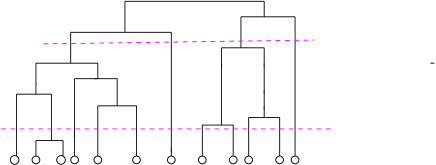
FIG. 2.: A typical dendogram. In the divisive algorithm, one explores from top to bottom while for a agglomerative method, one goes from the bottom to the top. The number of communities is given by the number of intersection points of the horizontal dashed lines with the dendogram at different levels. The circles represent the nodes.

2 A measure of the community structure identification

Applying either of the above algorithms it may be possible to divide the network into communities. Even the random graph with no community structure may be separated into many classes. One needs to have a measure to see how good the obtained structure is. Also, the dendogram represents communities at all levels from a single to as many as the number of nodes and one should have an idea at which level the community division has been most sensible.

In case the network has a fixed well known community structure, a quantity to measure the performance of the algorithm for the community detection may be the fraction of correctly classified nodes.

The other measure, known as the modularity of the network, can be used when there is no ad hoc knowledge about the community structure of the network. This is defined in the following way [50]. Let there be $k$ communities in a particular network. Then $e_{ij}$ is the fraction of edges which exist between nodes belonging to communities $i$ and $j$; clearly it is a $k\times k$ matrix. The trace $Tr(e)=\Sigma e_{ii}$ then gives the fraction of all edges in the network that connect vertices in the same community and a good division into communities should give a high value of the trace. However, simply the trace is not a good measure of the quality of the division as placing all nodes in a single community will give trivially $Tr(e)=1$. Let us now take the case when the network does not have a community structure; in this case links will be distributed randomly. Defining the row (or column) sums $\alpha_{i}=\Sigma_{j}e_{ij}$, one gets the fraction of edges that connect to vertices in community $i$. The expected number of fraction of links within a partition is then simply the probability that a link begins at $i$, $\alpha_{i}$, multiplied by the fraction of links that end at a node in $i,\alpha_{i}$. So the expected number of intra-community links is just $\alpha_{i}\alpha_{i}$. A measure of the modularity is then

$$Q=\Sigma_{i}(e_{ii}-\alpha_{i}^{2}),$$ (10)

which calculates the fraction of edges which connect nodes of the same type minus the same quantity in a network with identical community division but random connections between the nodes. If the number of within-community edges is no better than random, $Q=0$. The modularity plotted at every level of the bifurcation would indicate the quality of the detection procedure and at which level to look at to see the best division where $Q$ has a maximum value.

There are some typical networks to which the community detection algorithms are applied to see how efficient it is. Most of the methods are applied to an artificial computer generated graph to check its efficiency. Here 128 nodes are divided into four communities. Each node has $k=16$ neighbours of which $k_{out}$ connections are made to nodes belonging to other communities. The quality of separation into communities here can be measured by calculating the number of correctly classified nodes. All available detection algorithms work very well for $k_{out}\leq 6$ and the performance becomes poorer for larger values. A comparative study of application of different algorithms to this network has been made by Danon et al [51].

A popular network data with known community structure which is also very much in use to check or compare algorithms is the Zachary’s karate club (ZKC) data. Over the course of two years in the early 70’s, Wayne Zachary observed social interactions between the members of a karate club at an American university [52]. He constructed network of ties between members of the club based on their social interactions both within and outside the club. As a result of a dispute between the administrator and the chief karate teacher the club eventually split into two. Interestingly, not just two, but upto five communities have been detected in some of the algorithms.

Community structure in jazz network has also been studied. In this network, musicians are the nodes and two musicians are connected if they have performed in the same band. In a different formulation, the bands act as nodes and have a link if they have at least one common musician. This was studied mainly in [53].

The American college football network is also a standard network where community detection algorithms have been applied. This is a network representing the schedule of games between American college football teams in a single season. The teams are divided into groups or “conferences” and intra-conference groups are more frequent than inter-conference games. The conferences are the communities, so that teams belonging to the same conference would play more between themselves.

Community detection algorithms have been applied to other familiar social networks like collaboration and e-mail networks as well as in several non-social networks.

B Some novel community detection algorithms

The method of GN to detect the communities typically involves a time of the order of $N^{2}M$, where $N$ is the number of nodes and $M$ the number of edges. This is considerably slow. Several other methods have been proposed although none of them is really ‘fast’. Some of these methods are just variants of the divisive method of GN (i.e., edge removal by a certain rule) and interested readers will find the details in references [50, 54, 55]. Here we highlight those which are radically different from the GN method.

Optimisation methods

Newman [56] suggested an alternative algorithm in which one attempts to optimise the splitting for which $Q$ is maximum. However, this is a costly programme as the number of ways in which $N$ vertices can be divided into $g$ non-empty groups is given by Stirling’s number of the second kind $S_{N}^{(g)}$ and the number of distinct community division is $\Sigma_{g=1}^{N}S_{N}^{(g)}$. It increases at least exponentially in $N$ and therefore approximate methods are required. In [56], a greedy agglomerative algorithm was used. Starting from the state where each node belongs to its own cluster, clusters are joined such that the particular joining results in the greatest increase in $Q$. In this way a dendogram is obtained and the corresponding $Q$ values are calculated. Community division for which $Q$ is maximum is then noted. The computational effort involved in this method is $O((M+N)N)$. For small networks, the GN algorithm is better but for large networks this optimisation method functions more effectively. Applications of this method has been done for the ZKC and the American football club networks.

Duch and Arenas [57] have used another optimisation method which is local using extremal optimisation. In this local method, a quantity $q_{r}$ for the $r$th node is defined

$$q_{r}=\kappa_{i(r)}-k_{r}\alpha_{i(r)},$$ (11)

where $\kappa_{i(r)}$ is the number of links that a node $r$ belonging to a community $i$ has with nodes in the same community and $k_{r}$ is the degree of node $r$, $\alpha_{i(r)}$ is the fraction of edges connected to $r$ having either or both end in the community $i$. Note that $q_{r}$ is just the contribution to $Q$ (eq. (10)) from each node in the network, given a certain partition into communities, and $Q=\frac{1}{2N}\Sigma_{r}q_{r}$. Rescaling the local variables $q_{r}$ by $k_{r}$, a proper definition for the contribution of node $r$ to the modularity can be obtained. In this optimisation method, the whole graph is initially split into two randomly. At every time step, the node with the lowest fitness $\lambda_{r}=q_{r}/k_{r}$ is moved from one partition to another. The process is repeated until an optimal state with a maximum value of $Q$ is reached. After that all the inter-partition links are deleted and the optimisation procedure applied to the resulting partitions. The process is continued till the modularity $Q$ cannot be improved anymore. Applications were made to the ZKC, jazz, e-mail, cond-mat and biological networks. In each case it gives a higher modularity value compared to that of the GN method.

Spectral methods

The topology of a network with $N$ vertices can be expressed through a symmetric $N\times N$ matrix $L$, the Laplacian matrix, where $L_{ii}=k_{i}$ (degree of the $i$th node) and $L_{ij}$ are equal to $-1$ if $i$ and $j$ are connected and zero otherwise. The column or row sum of $L$ is trivially zero. A constant vector, with all its elements identical will thus be an eigenvector of this matrix with eigenvalue zero.

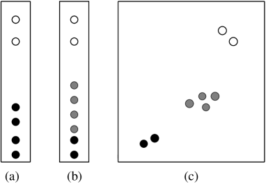
FIG. 3.: (a) The structure of the first non-trivial eigenvector when there are only two communities. (b) An example of a case with three communities, now the first nontrivial eigenvector has a structure with fuzziness when the components corresponding to two communities are pretty close (shown in gray and black). (c) When the first two non-trivial eigenvectors are projected on a two dimensional space, the three communities are clearly shown.

For a connected graph, the eigenvectors are non-degenerate. Since $L$ is real-symmetric, the eigenvectors are orthogonal. This immediately implies that the sum of the components of the other eigenvectors are zero as the first one is a constant one. In case the number of subgraphs is equal to two, there will be a clear cut bifurcation in the eigenvector; components of the second (first non-trivial) eigenvector are positive for one subgraph and negative for the other. This is the spectral bisection method which works very well when only two communities are present, e.g., in the case of the ZKC network.

For more than two subgraphs, the distinction may become fuzzy (see Fig. 3). In this case, a few methods have been devised recently [58, 59, 60]. The eigenvectors of $L$ with non-zero eigenvalues are the non-trivial eigenvectors. If there is a network structure with $m$ communities, there will be $m-1$ nontrivial eigenvectors with eigenvalues close to zero and these will have a characteristic structure: the components corresponding to nodes within the same cluster have very similar values $x_{i}$. If the partition is sharp, the profile of each eigenvector, sorted by components, is step like. The number of steps in the profile corresponds to the number of communities. In case the partition is not so sharp, and the number of nodes is high, it is difficult to arrive at a concrete conclusion by just looking at the first nontrivial eigenvector. The method is then to combine information from the first few, say $D$, nontrivial eigenvectors. Consider an enlarged $D$ dimensional space where the components of these eigenvector are projected (i.e., the coordinates of the points in this space correspond to the values of the components of the eigenvectors for each node). The points one gets can now be treated as the “positions” of the nodes and nodes belonging to the same community are clustered in this space. Donetti and Munoz [59] used an agglomerative method to detect communities from this $D$ dimensional space. The choice of $D$, the number of eigenvectors to be used, is an important question here. One can fix a value of $D$, and find out the optimal value of $Q$ - the $D$ value corresponding to the best optimal value of $Q$ may be the ideal choice. It was observed that $D$ is of the order of the number of communities in the network.

Instead of the Laplacian matrix, one can also take another matrix, $X=K-A$ where $K$ is the diagonal matrix with elements $k_{ii}=\Sigma_{j=1}^{N}a_{ij}$ and $a_{ij}$ the elements of the adjacency matrix $A$. Here instead of zero eigenvalue, the normal matrix $X$ has largest eigenvalue 1 associated with the trivial eigenvector. This matrix has been used by Capocci et al [58] for networks with weighted edges successfully. It has been tested on a directed network of word association where the method has been modified slightly to take into account the directedness of the edges.

Methods based on dissimilarity

Two vertices are said to be similar if they have the same set of neighbours other than each other. Exact similarity is rare, so one can define some dissimilarity measure and find out the communities using this measure. One of these measures is called the Euclidean distance discussed in [47]. Recently, another measure based on the differences in their “perspective” was done. Taking any vertex “$i$”, the distance $d_{ik}$ to a vertex “k” can be measured easily. Taking another node “$j$”, one can measure $d_{jk}$. If the nodes belong to the same community, then the difference $[d_{ik}-d_{jk}]^{2}$ is expected to be small. The dissimilarity index $\lambda_{ij}$ was defined by Zhou [61] as

$$\lambda_{ij}=\frac{\sqrt{\Sigma_{k}[d_{ik}-d_{jk}]^{2}}}{N-2}.$$ (12)

The algorithm is a divisive one involving a few intricate steps and has been successfully applied to many networks.

Another local method

Bagrow and Bollt [62] have suggested a local method in which, starting from a particular node, one finds out $k^{(l)}$, the number of its $l$th nearest neighbours at every stage $l=0,1,2,...~{}$. By definition, $k^{(0)}=1$. The cumulative number of degrees $K^{(l)}=\Sigma k^{(l)}$ is also evaluated here. The ratio $K^{(l+1)}/K^{(l)}$ is compared to a preassigned quantity $\alpha$ and in case the ratio is less than $\alpha$, the counting is terminated and all nodes upto the $l$th neighbourhood are listed as members of the starting node’s community.

C Community detection methods based on physics

A few methods of detecting communities are based on models and methods used in Physics.

Network as an electric circuit

Wu and Huberman [63] have proposed a method by considering the graph to be an electric circuit. Suppose it is known that nodes A and B belong to different communities. Each edge of the the graph is regarded as a resistor and all edges have identical resistance. Let a battery connect A and B such that the voltages at A and B are 1 and 0 respectively. Now the graph is simply an electric circuit with a current flowing through each resistor. By solving Kirchoff’s equations one can obtain the voltage at each node. Choosing a threshold value of the voltage (which obviously lies between 0 and 1), one then decides whether a node belongs to the community containing A or that containing B. It is easy to see how this method works: first suppose that there is a node C which is a leaf or peripheral node, i.e., connected to a single node D. No current flows through CD and therefore C and D have the same voltage and belong to the same community. Next consider the case when C is connected to nodes D and E. Since the resistance is same for all edges, $V_{c}=(V_{D}+V_{E})/2$. Hence if both D and E belong to the same community (i.e., they both have high or low voltages), C also has a comparable voltage and belongs to the same community. If, however, $V_{D}$ and $V_{E}$ are quite different and D and E belong to different communities then it is hard to tell which community C belongs to. This is close to reality, a node has connection with more than one community. In general, when C is linked to $n$ other nodes with voltages $V_{1},V_{2},...,V_{n}$, $V_{c}=\Sigma V_{i}/n$. Hence if most of its neighbours belong to a particular community, C also belongs to it. The method works in linear time.

When it is not known initially that two nodes belong to two different communities, one can randomly choose two nodes and repeat the process of evaluation of communities a large number of times. Chances that the detection is correct is fifty percent. However, this probability will be greater than half if these two initial nodes are chosen such that they are not connected. Majority of the results would then be regarded as correct. Applications have been made to the ZKC and the College football club networks.

Application of Potts and Ising models:

The $q$ state Potts model in Physics is a model in which the spin at site $i$ can have a value $\sigma_{i}=1,2,....,q$. If two spins interact in such a way that the energy is minimum when they have the same value, we have the ferromagnetic Potts model. Potts model has well known application for graph colouring problem, where each colour corresponds to a value of the spin. For community detection also, the method can be similarly applied. Reichardt and Bornholdt [64] have used the Potts model Hamiltonian

$$H=-J\Sigma_{i,j}\delta_{\sigma_{1},\sigma_{2}}+\gamma\Sigma_{\sigma}^{q}\frac{n_{\sigma}(n_{\sigma}-1)}{2},$$ (13)

where $n_{\sigma}$ is the number of spins having spin $s$. Here the first term is the standard ferromagnetic Potts model and in absence of the second term it favours a homogeneous distribution of spins which minimises the ferromagnetic term. However, one needs to have diversity and that is incorporated by the second term. If there is only one community it will be maximum and if spin values are more or less evenly distributed over all nodes it will be minimum.

When $\gamma$ is set equal to the average connection probability, then both the criteria that (a) within a community the connectivity is larger than the average connectivity, and that (b) the average connectivity is greater than the inter-community connectivity, are satisfied. With this value of $\gamma$ and $J=1$, the ground state was found out by the method of simulated annealing. The communities appeared as domains of equal spin value near the ground state of the system. Applications to computer generated graphs and biological networks were made successfully and the method can work faster than many other algorithms.

In another study by Guimerà et al [65] in which the Potts model Hamiltonian is used again, although in a slightly different form, an interesting result was obtained. It was shown that networks embedded in low-dimensional spaces have high modularity and that even random graphs can have high modularity due to fluctuations in the establishment of links. The authors argue that like the clustering coefficient, modularity in complex networks should also be compared to that of the random graph.

Son et al [66] have used a Ising model Hamiltonian to detect the community structure in networks. The Ising model is the case when the spins have only two states, usually taken to be $\sigma=\pm 1$. This method can be best understood in the context of the Zachary karate club case. Here two members started having difference and the club members eventually got polarised. In this case, the authors argue, the members will try to minimise the number of broken ties, or in other words, the breakup of ties should be in accordance to the community structure. Thus the community structure may be found out by simulating the breakup caused by an enforced frustration among nodes. The breakup is simulated by studying the ferromagnetic random field Ising model which has the Hamiltonian

$$H=-\frac{1}{2}\Sigma_{i,j}J_{ij}\sigma_{i}\sigma_{j}-\Sigma_{i}B_{i}\sigma_{i},$$ (14)

where $\sigma_{i}$ is the Ising spin variable for the $i$th node and the spins interact ferromagnetically with strength $J_{ij}$ and $B$ is the random field. $J_{ij}$ is simply equal to the elements of the adjacency matrix, can be 1 or 0 for unweighted networks and equal to the weights for a weighted graph. The ferromagnetic interaction, as in the Potts case, represents the cost for broken bonds. The conflict in the network (e.g., as raised in the ZKC) is mimicked in the system by imposing very strong negative and positive fields for two nodes (in the ZKC case, these nodes should correspond to the instructor and administrator). The spins with the same signs in the ground state then belong to the same community. The method was applied to the Zachary Karate club network and the co-authorship networks with a fair amount of success. It indicated the presence of some nodes which were marginal in the sense that they did not belong to a community uniquely.

D Overlap of communities and a network at a higher level

Division of a society into communities may be done in many ways. If the criteria is friendship, it is one, while if it is professional relation it is another. A node in general belongs to more than one community. If one focuses on an individual node, it lies at the center of different communities (see Fig. 4). Within each of these communities also, there are subgraphs which may or may not have overlaps. Considering such a scenario, Pallà et al [67] developed a new concept, the “network of communities”, in which the communities acted as nodes and the overlap between communities constituted the links.

Here a community was assumed to consist of several complete subgraphs ($k$ cliques [68]) which tend to share many of their nodes and a single node belongs to more than one community. Pallà et al [67] defined certain quantities:
(i) The membership number $m$ which is the number of communities a node belongs to
(ii) Size of a community $n_{s}$ which is the number of nodes in it
(iii) Overlap size $s^{\alpha,\beta}$, the number of nodes shared by communities $\alpha$ and $\beta$.
Two quantities related to the network of communities were also defined:
(i) Community degree $k_{c}$ - the number of communities a community is attached to.
(ii) Clustering coefficient of the community network.

A method was used in which the $k$ cliques are first located and then the identification is carried out by a standard analysis of the clique-clique overlap matrix [68]. Identification and the calculation of the distributions for the quantities $m$, $n_{s}$, $s^{\alpha,\beta}$ and $k_{c}$ were done for the co-authorship, word association and biological networks.

FIG. 4.: A node (black circle) belonging to different communities. i A particular community, e.g., the community of colleagues, may again contain subcommunities P,M,S etc.

The community size distributions $P(n_{s})$ for the different real networks appear to be power law distributed ($n_{s}^{-\tau}$) with the value of the exponent $\tau$ between $-2$ and $-2.6$. At the node level, the degree distribution is often a power law in many networks. Whether at a higher level, i.e., at the community level it also has the same organisation is the important question. The degree distribution of the communities showed an initial exponential decay followed by a power law behaviour with the same exponent $\tau$.

The distribution of the overlap size $s^{ov}$ and the membership number $m$ also showed power law variations with both the distributions having a large exponent for the collaboration and word association networks. This shows that there is no characteristic overlap size and that a node can be the member of a large number of communities.

The clustering coefficients of the community networks were found out to be fairly large, e.g., 0.44 for the cond-mat collaboration network, showing that two communities overlapping with a given community has a large probability of overlapping with each other as well.

Preferential attachment of communities

As the community degree distribution (or the size distribution) is scale-free, the next question which arises is what happens to a new node which joins a community, i.e., what is the attachment rule chosen for the new node as regards the size and degree of the communities [69]?

To determine the attachment probability with respect to any property $\rho$, the cumulative distributions $P(\rho)$ at times $t$ and $t+1$ are noted. Let the un-normalised $\rho$ distribution of the chosen objects during the time interval $t$ and $t+1$ be $w_{t\to t+1}(\rho)$. The value of $w_{t\to t+1}(\rho^{*})$ at a given $\rho^{*}$ equals the number of objects chosen which have a $\rho$ value greater than $\rho^{*}$. If the process is uniform, then objects chosen with a given $\rho$ are chosen at a rate given by the distribution of $\rho$ amongst the available objects. However, if the attachment mechanism prefers high (low) $\rho$ values, then objects with high (low) $\rho$ are chosen with a higher rate compared to the distribution $P(\rho)$. In real systems, the application of the method indicated that rather than a uniform attachment there is a preferential attachment even at the higher level of networks.

VIII Models of social network

In this section we discuss some models of social network which particularly aim at reproducing the community structure and/or positive assortativity. We also review some dynamical models which show rich phase transitions.

A Static models

By static models we mean a social model where the existing relations between people remain unchanged while new members can enter and form links and the size of the system may grow. Examples are collaboration networks where existing links cannot be rewired.

Newman and Park [46] have constructed a model which has a given community division. The aim is to show that it has positive assortativity. Here it is assumed that members belonging to the same community are linked with probability $p$ similar to a bond percolation [70] problem. An individual may be attached to more than one community, and the number of members in a community is assumed to be a variable here.

The assortativity coefficient $r$ was calculated here in terms of $p$ and the moments of the distributions of $m$ (the number of communities to which a member belongs) and $s$ (the community size). The theoretical formula was applied to real systems after estimating the distributions by detecting communities using standard algorithms. The value of $p$ was calculated by dividing the number of edges in the network by the total number of possible within-group edges. The theoretical value of $r$ for the co-authorship network turns out to be 0.145 which is within the statistical error of the real value $0.174\pm 0.045$.

Another model was proposed by Catanzaro et al [71] to reproduce the observations of a specific database, the cond-mat archive of preprints. This network of co-authors was found to be scale-free with positive assortativity. In the model the preferential attachment scheme was used with some modification: the new node gets linked to an existing node with preferential attachment but with a probability $p$. Two existing nodes with degree $k_{1}$ and $k_{2}$ could also get linked stochastically with the probability being proportional to $(1-p)f(|k_{1}-k_{2}|)$. $f(x)$ was chosen to be decaying with $x$ either exponentially or as a inverse power law. It was shown that by tuning the parameter $p$, one could obtain different values of the exponents for the degree distribution, clustering coefficient, assortativity and betweenness. The results agree fairly well for all the quantities of the actual network except the clustering coefficient.

Bogũna et al [72] have used the concept of social distance in their model. A set of quantities $h^{i}_{n}$ for the $n$th individual is used to represent the characteristic features of individuals like profession, religion, geographic locations etc. Social distance between two individuals $n$ and $m$ with respect to characteristic $i$ can be quantified by the difference of $h_{n}^{i}$ and $h_{m}^{i}$. It is assumed that two individuals with larger social distance will have a lesser probability of getting acquainted. If the social distance with respect to the $i$th feature is denoted by $d_{i}(h_{n}^{i},h_{m}^{i})$, then a connection probability is defined as

$$r_{i}(h_{n}^{i},h_{m}^{i})=\frac{1}{1+[b_{i}^{-1}d_{i}(h_{n}^{i},h_{m}^{i})]^{\alpha}},$$ (15)

where $\alpha$ is a parameter measuring homophily, the tendency of people to connect to similar people and $b_{i}^{-1}$ is a characteristic scale. The total probability of a link to exist between the two individuals is a weighted sum of these individual probabilities

$$r(h_{n},h_{m})=\Sigma_{i}w_{i}r_{i}(h_{n}^{i},h_{m}^{i}).$$ (16)

The degree distribution, the clustering coefficient and the assortativity (in terms of $\langle k_{nn}\rangle$) were obtained analytically for the model and also compared to simulation results. The resulting degree distribution had a cutoff, the clustering coefficient showed increase with $\alpha$ and the assortativity was found out to be positive. The model also displayed a community structure when tested with the GN algorithm.

In the model proposed by Wong et al [73], nodes are distributed in a Euclidean space and the connection probabilities depend on the distance separating them. Typically, a neighbourhood radius is defined within which nodes are connected with a higher probability. For chosen values of the parameters in the scheme, graphs were generated which showed community structure and small world effect.

A hierarchical structure of the society has been assumed by Motter et al [74] in their model in which the concept of social characteristics is used. Here a community of $N$ people are assumed to have $H$ relevant social characteristics. Each of these characteristic defines a nested hierarchical organisation of groups, where people are split into smaller and smaller subgroups downwards in this nested structure (Fig. 5). Such a hierarchy is characterised by the number $l$ of levels, the branching ratio $b$ at each level and the average number $g$ of people in the lowest group.

FIG. 5.: A hierarchical structure of human population obtained using a single characteristic feature. People belonging to the same lowest group (ellipse) have social distance 1 and the distance increases as one goes up in the hierarchy. The maximum distance in this case is $l=4$.

Here also distance factors corresponding to each feature can be defined and it is assumed that the distances are correlated, i.e., two individuals are expected to be different (similar) to each other in the same degree with respect to different characteristics. Connection probability decreases exponentially with the social distance and links are generated until the number of links per person reaches a preassigned average value. Networks belonging to the random and regular class are obtained for extreme values of the parameters and in between there is a wide region in which social networks fall.

A growing model of collaboration network to simulate the time dependent feature of the link length distribution observed in [22] has been proposed recently by Chandra et al [75]. Here the nodes are embedded on a Euclidean two dimensional space and an incoming node $i$ gets attached to (a) its nearest neighbour $j$, (b) to the neighbours of $j$ with a certain constant probability and (c) to other nodes with a time dependent probability. Step (a) takes care of the proximity bias, step (b) ensures high clustering and step (c) takes care of the fact that long distance collaborations increase in time thanks to rapid progress in communication. The link length distributions obtained from the simulations are consistent with the observed results and the model also gives a positive assortativity.

B Dynamical models

Dynamical models allow the links to change in time whether or not the network remains constant in size. This is close to reality as human interactions are by no means static [76, 77]. These models are applicable to cases where direct human interactions are involved.

In Jin et al [78], the model consists of a fixed number of members and links may have a finite lifetime. Here it is assumed that the probability of interaction between two individuals depends on their degrees and is enhanced by the presence of a mutual friend. A cutoff in the number of acquaintances ensures that the total number of links has an upper bound. The strength $s_{ij}$ of a tie between individuals $i$ and $j$ is a function of the time $t$ since they last met; $s_{ij}\sim\exp(-\kappa t)$. Starting with a set of individuals with no links, edges are allowed to appear with a small value of $\kappa$ close to zero. When the network saturates, $\kappa$ is set to a larger value and the evolution of the network studied. The resulting network shows features of large clustering and community structure for realistic range of values of $\kappa$.

A somewhat similar model has been proposed by Ebel et al [79] where new acquaintances are initiated by mutual friends with the additional assumption that a member may leave the network with probability $p$. All its links are deleted in that case. The finite lifetime of links brings the network to a stationary state which manifests large clustering coefficients, small diameter and scale free or exponential degree distribution depending on the value of $p$.

Another model which aims at forming communities is due to Grönlund and Holme [80] who construct a model based on the assumption that individual people’s psychology is to try to be different from the crowd. This model is based on the agent based model known as the seceder model [81]. It involves an iterative scheme where the number of nodes remains constant and the links are generated and rewired during the evolution. Networks generated by this algorithm indeed showed community structure and small world effect while the degree distribution had an apparent exponential cutoff. The clustering coefficient was found to be much higher than the corresponding random network while the assortativity coefficient $r$ showed a positive value.

Some of the dynamic models are motivated by the model proposed by Bonabeau et al [82] in which agents are distributed randomly in a $L\times L$ lattice and assigned a “fitness” variable $h$. The agents perform random walk on the lattice and during an interaction of agents $i$ and $j$, the probability that $i$ wins over $j$ is $q_{i}$ given by

$$q_{i}=\frac{1}{1+\exp(\eta(h_{i}-h_{j}))}.$$ (17)

If the fluctuation $\sigma$ of the $q_{i}$ values is small, the resulting society is egalitarian while for large values of $q$, it is a society with hierarchical structure. In the model the individuals occupy the lattice with probability $p$. A phase transition is observed as the value of $p$ is changed (in a slightly modified model where $\eta$ is replaced by $\sigma$). Gallos [83] has shown that when a model with random long distant connections is considered the phase transition remains with subtle differences in the behaviour of the distribution of $q$.

In another variation of the Bonabeau model, Ben-Naim and Redner [84] allow the fitness variable to increase by interactions and decline by inactivity. The latter occurs with a rate $r$. The rate equation for the fraction of agents with a given fitness was solved to show a phase transition as $r$ is varied; with $r\geq 1$, one has a society with a single class and for $r\geq 1$, a hierarchical multiple class society can exist. In the latter case, the lower class is destitute and the middle class is dynamic and has a continuous upward mobility.

Individuals are endowed with a complex set of characteristics rather than a single fitness variable. Models which allow dynamics of these social characteristics have also been proposed recently. Transitions from a perfect homogeneous society to a heterogeneous society has been found in the works of Clemmy et al [85] and Gonzalez-Avella et al [86].

Let each trait take any of the integral values $1,2,...,q$. When individuals have nearest neighbour interactions and the initial traits follow a Poisson distribution, the non-uniformity in the traits can drive the system to a heterogeneous state at $q=q_{c}$ [87]. Klemm et al found that on a small world network, the transition point $q_{c}$ shifts towards higher values as the disorder (fraction of long range bonds) is enhanced and the transition disappears in a scale-free BA network in the thermodynamic limit. In [86], the additional influence of an external field has been considered.

Shafee [88] has considered a spin glass like model of social network which is described by the Hamiltonian

$$H=-\Sigma_{i,k,a,b}J^{ab}_{ik}s^{a}_{i}s^{b}_{k}-\Sigma_{i,a}h_{i}^{a}s^{a}_{i},$$ (18)

where $s^{a}_{i}$ is the state of the $i$th agent with respect to trait $a$, $J^{ab}_{ik}$ are the interaction between different agents and $h_{i}^{a}$ an external field. Zero temperature Monte Carlo dynamics is then applied to the system. However, the simulations were restricted to systems of very small sizes. Results showed either punctuated equilibrium or oscillatory behaviour of the trait values with time.

IX Is it really a small world? Searching: post Milgram

Although Milgram’s experiments have been responsible for inspiring research in small world networks, they have their own limitation. The chain completion percentage was too low - in the first experiment it was just five. The later experiment had a little better success rate but this time the recruit selection was by no means perfectly random. Actually, a number of subtle effects can have profound bearing on what can be termed “searching in small worlds”. First, although the network may have a small world property, searches are done mainly locally - the individual may not know the global structure of the network that would help her or him to find out the shortest path to a target node. Secondly, many factors like the race, income, family connections, job connections, friend circle etc. determine the dynamics of the search process. Quite a few experiments in this direction are being carried out currently. Some theoretical approaches have also been proposed for the searching mechanism.

A Searching in small world networks

The first theoretical attempt to find out how a search procedure works in a small world network was made by Kleinberg [24] in which it was assumed that the nodes were embedded on a two dimensional lattice. Each node was connected to its nearest neighbour and a few short cuts (long range connections) were also present to facilitate the small world effect. The probability that two nodes at an Euclidean distance $l$ had a connection was taken to be $P(l)\sim l^{-\alpha}$. The algorithm used was a “greedy algorithm”, i.e., each node would send the message to one of its nearest neighbours, and look for the neighbour which takes it closest to the target node. Here the source and target nodes are random. Interestingly, it was found that only for a special value of $\alpha=2$, the time taken (or the number of steps) scaled as $\log(N)$, while for all other values it varied sublinearly with $N$. This result, according to [24] could be generalized to any lattice of dimension $d$ and there always existed a unique value of $\alpha=d$ where short paths between two random nodes could be found out. Navigation on the WS model [89] and a one-dimensional Euclidean network [90] agreed perfectly with the above picture.

The above results indicate that although the network may have small average shortest paths globally, it does not necessarily mean that short chains can be realised using local information only.

B Searching in scale-free graphs

In a scale free network with degree distribution given by $P(k)\sim k^{-\tau}$, one can consider two kinds of searches, one random and the other one biased. In the latter, one has the option of choosing neighbouring nodes with higher degree which definitely makes the searching process more efficient.

Adamic et al [91] have assumed that apart from the knowledge about one’s nearest neighbours, each member also has some knowledge about the contacts of the second neigbours. Using this assumption, the average search length $s$ in the random case is given by

$$s\sim N^{3(1-2/\tau)}.$$ (19)

Only for $\tau=2$, the search length is $O(\ln(N)^{2})$. The corresponding expression for the biased search, when nodes with larger degree are used, is

$$s\sim N^{2-4/\tau}.$$ (20)

Simulations were done with random and biased search mechanisms where a node could scan both its first and second neighbours. The results for $\tau\neq 2$ indeed yielded shortest paths which scale sublinearly with $N$, although in a slower manner compared to the theoretical predictions.

C Search in a social network

A social network comprising of people whose links are based on friendship or acquaintance can be thought of as a network where the typical degree of each node is $k=O(10^{3})$. Hence the number of second neighbours should be of $k^{2}$ and therefore, ideally in two steps one can access $10^{6}$ number of other people and the search procedure would be complete if the order of total population is similar. Even if the degree is one order lesser, the number of steps is still quite small and search paths can be further shortened by taking advantage of highly connected individuals. However, there is a flaw in this argument as there is a considerable overlap of the set of one’s friends and that of one’s friends’ friends.

It is expected that the participants in a real searching procedure would like to take advantage of certain features like geographical proximity or similarity of features like profession and hobbies etc. In this background the hierarchical structure of the social network is extremely significant (Fig. 5).

Watts et al [92] have considered a hierarchical model in which the individuals are endowed with network ties and identities by a set of characteristics as described in sec. VIII A. Distance between individuals are calculated as the height of their lowest common ancestor level in the hierarchy.

The probability of acquaintance between two individuals is assumed to be proportional to $\exp(-\alpha x)$ where $\alpha$ is the measure of homophily and $x$ the social distance. Unlike [74], here it is assumed that the distance between two individuals for two different features are uncorrelated. One can consider the minimum distance $y_{ij}$, the smallest of the $x_{ij}$’s corresponding to all the social features, to be sufficient to connote affiliation.

It is assumed that the individual who passes the message knows only its own coordinates, its neighours coordinates and the coordinates of the target node. Thus the search process is based on partial information, information about social distance and network paths are both only locally known.

In this work one important aspect of the original experiments by Milgram and his coworkers was brought under consideration, that most of the search attempts failed but when it was successful it took only a few steps. Introducing a failure probability $p$ that a node fails to carry forward the message, it is to be noted that if the probability of a successful search of length $s$ is $r$, it must satisfy $q=(1-p)^{s}\geq r$. This gives an upper limit for $s$; $s\leq\log(r)/\log(1-p)$. In the simulations, the number of traits $H$ and $\alpha$ were varied keeping $p=0.25$ and $r=0.05$ fixed (these values are in accordance with realistic values which gives $s\leq 10.4$). The values of the average number of nearest neighbours and branching ratio were also kept constant. A phase diagram in the $H-\alpha$ plane showed regions where the searching procedure can be successful. It showed that almost all searchable networks display $\alpha>0$ and $H>1$. The best performance, over the largest range of $\alpha$, is achieved for $H=2$ or $3$. In fact the model could be tuned to reproduce the experimental results of Milgram ($s\sim 6.7$).

D Experimental studies of searching

A few projects to study searching in social networks experimentally have been initiated recently. Dodds et al [93] have conducted a global, Internet based social search by registering participants online. Eighteen target persons from 13 countries with varied occupation were randomly selected and the participants were informed that their task was to help relay a message to their allocated target by passing the message to a social acquaintance whom they considered closest to the target. One fourth of the participants provided their personal information and it showed that the sample was sufficiently representative of the general Internet using population. The participants also provided data as to on what basis he or she chose the contacts’ name and e-mail address; in maximum cases they were friends, followed by relatives and colleagues.

The links in this experimental network showed that geographical proximity of the acquaintance to the target and similarity of occupation were the two major deciding factors behind their existence. Many of the chains were terminated and not completed as in Milgram’s experiment and the reason behind it was mainly lack of interest or incentive. In total, 384 chains were completed (nearly 100000 persons registered in the beginning). It was also found that when chains did complete, they were short, the average length $s$ being 4.05. However, this is a measure for completed chains only, and the hypothetical estimate in the limit of zero attrition comes out to be $s=7$.

In another study, Adamic and Adar [94] derived the social network of e-mails at HP laboratories from the e-mail logs by defining a social contact to be someone with whom at least six e-mails have been exchanged both ways over an approximate period of three months. A network of 430 individuals was generated and the degree distribution showed an exponential tail. Search experiments were simulated on this network. Three criteria for sending messages in the search strategy was tested in this simulation; degree of the node, closeness to the target in the organisational hierarchy and location with respect to the target.

In a scale-free network, seeking a high degree node was shown to be a good search strategy [91]. However, in this network, which has an exponential tail, this does not work out to be effective. This is because most of the nodes do not have a neighbour with high degree. The second strategy of utilising the organising hierarchy worked much better showing that the hierarchical structure in this network is quite appropriate. The probability of linking as a function of the separation in the organisational hierarchy also showed consistency with an exponential decay as in [92]. The corresponding exponent $\alpha$ has a value = 0.94 and is well within the searchable region identified in [92].

The relation between linkage probability and distance $r$ turned out to be $1/r$ in contrast to $1/r^{2}$ where the search strategy should work best according to [24]. Using geographical proximity as a search strategy gave larger short paths compared to the search based on organisational hierarchy, but the path lengths were still ‘short’.

A similar experiment was conducted by Liben-Nowell et al [95], using a real world friendship network to see how the geographical routing alone is able to give rise to short paths. In this simulated experiment, termination of chains was allowed. Chain completion was successful in thirteen percent cases with average search length a little below 6.

X Endnote

Study of social networks has great practical implications with respect to many phenomena like spreading of information, epidemic dynamics, behaviour under attack etc. In these examples, the analysis of the corresponding networks can help in making proper strategies for voting, vaccination or defence programmes. In this particular review, we have highlighted mainly the theoretical aspects of social networks like structure, modelling, phase transitions and searching. Social networks has emerged truly as an interdisciplinary topic during recent times and the present review is a little biased as it is from the viewpoint of a physicist.

XI Appendix: The Indian railways network

The Indian railways network (IRN) is more than 150 years old and has a large number of stations and trains (running at both short and long distances). In the study of the IRN [45], a coarse graining was made by selecting a sample of trains, and the stations through which these run. The total number of trains considered was 579 which run through 587 stations. Here the stations represent the ‘nodes’ of the graph, whereas two arbitrary stations are considered to be connected by a ‘link’ when there is at least one train which stops at both the stations. These two stations are considered to be at unit distance of separation irrespective of the geographical distance between them. Therefore the shortest distance $\ell_{ij}$ between an arbitrary pair of stations $s_{i}$ and $s_{j}$ is the minimum number of different trains one needs to board on to travel from $s_{i}$ to $s_{j}$. Smaller subsets of the network were also considered to analyse the behaviour of different quantities as a function of the number of nodes. The average distance between an arbitrary pair of stations was found to depend only logarithmically on the total number of stations in the country as shown in Fig. 6.

FIG. 6.: The variation of the mean distance ${\cal D}(N)$ of 25 different subsets of IRN having different number of nodes $(N)$. The whole range is fitted with a function like ${\cal D}(N)=A+B\log(N)$ where $A\approx 1.33$ and $B\approx 0.13$. The inset shows the distribution Prob$(\ell)$ of the shortest path lengths $\ell$ on IRN. The lengths varied to a maximum of only five link lengths and the network has a mean distance ${\cal D}(N)\approx 2.16$.

Like other social networks, the IRN also showed a large clustering coefficient which also depends on the number of nodes (stations). For the entire IRN, the clustering coefficient is around 0.69, the value for the corresponding random graph being 0.11. The clustering coefficient as a function of the degree $k$ of a node showed that it is a constant for small $k$ and decreases logarithmically with $k$ for larger values.

The degree distribution $P(k)$ of the network, that is, the distribution of the number of stations $k$ which are connected by direct trains to an arbitrary station was also studied. The cumulative degree distribution $F(k)=\int_{k}^{\infty}P(k)dk$ for the whole IRN approximately fits to an exponentially decaying distribution: $F(k)\sim\exp(-\alpha k)$ with $\alpha$= 0.0085 (Fig. 7).

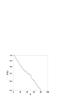
FIG. 7.: The cumulative degree distribution $F(k)$ of the IRN with the degree $k$ is plotted on the semi-logarithmic scale.

FIG. 8.: The variation of the average degree $\langle k_{nn}(k)\rangle$ of the neighbours of a node of degree $k$ with $k$ in the IRN. After some initial fluctuations, $\langle k_{nn}(k)\rangle$ remains almost same over a decade around $k$ = 30 to 300 indicating absence of correlations among the nodes of different degrees.

The average degree $\langle k_{nn}(k)\rangle$ of the nearest neighbours of a node with degree $k$ is plotted in Fig. 8 to check the assortativity behaviour of the network. This data is not very indicative. The assortativity coefficient $r$ is therefore calculated using eq. (4), which gives the value $r$ = -0.033. This shows that unlike social networks of class A and B, here the assortativity is negative.

REFERENCES

- [1] Wasserman S., Faust K., Social Network Analysis, Cambridge University Press, 1994
- [2] Watts D. J., Strogatz S. H., Nature 393 (1998) p. 440
- [3] Albert R., Barabási, A.-L., Rev. Mod. Phys. 74 (2002) p. 47
- [4] Barabási A.-L., Linked, Perseus, 2002
- [5] Dorogovtsev S. N., Mendes J. F. F., Evolution of Networks, Oxford University Press, 2003
- [6] Milgram, S., Psychology Today 1 (1967) p. 60; Travers J., Milgram S., Sociometry 32 (1969) p. 425
- [7] Erdös P., Rényi A., Publ. Math. 6 (1959) p. 290
- [8] Barabási, A.-L., Albert R., Science 286 (1999) p. 509
- [9] Freeman C., Sociometry 40 (1977) p. 35
- [10] Goh K.-I., Oh E., Kahng B., Kim D., Phys. Rev. E 67 (2003) p. 017101
- [11] Newman M. E. J., Phys. Rev. Lett. 89 (2002) p. 208701
- [12] Ebel H., Mielsch L-I., Berholdt S., Phys. Rev. E 66 (2002) p. 035103R
- [13] Barrat A., Weigt M., Eurphys. J. B 13 (2000) p. 547; Gitterman M., J. Phys A 33 (2000) p. 8373; textscKim B. J., Hong H, Holme P., Jeon G. S., Minnhagen P., Choi M. Y. Phys. Rev. E 64 (2001) p. 056135; Kim B. J., Hong H., Kim B. J., Choi M. Y. Phys. Rev. E 66 (2002) p. 018101
- [14] Huberman, B. A., Adamic L. A., Nature 401, (1999) p. 131
- [15] Masuda N., Miwa H., Konno N., Phys. Rev. E 71 (2005) p. 036108
- [16] Yook S.-H., Jeong H. Barabási A.-L., Proc. Natl. Acad. Sci. USA 99 (2002) p. 13382
- [17] Katz, J. S., Scientometrics 31 (1994) p. 31
- [18] Nagpaul P. S., Scientometrics 56 (2003) p. 403
- [19] Rosenblat T. S., Mobius M. M., Quart. J. Econ 121 (2004) p. 971
- [20] Gastner M. T., Newman M. E. J., cond-mat/0407680
- [21] Olson G. M., Olson J. S., Hum. Comp. Inter. 15 (2004) p. 139
- [22] Sen P., Chandra A.K., Basu Hajra K., Das P.K., physics/0511181
- [23] Waxman B., IEEE J. Selec. Areas Comm, SAC 6 (1988) p. 1617
- [24] Kleinberg J. M., Nature 406 (2000) p. 845
- [25] Jespersen S., Blumen A., Phys. Rev. E 62 (2000) p. 6270
- [26] Sen P., Chakrabarti B. K., J. Phys. A 34 (2001) p. 7749.
- [27] Moukarzel C. F., de Menezes M. A., Phys. Rev. E 65 (2002) p. 056709
- [28] Sen P., Banerjee K., Biswas T., Phys. Rev. E 66 (2002) p. 037102
- [29] Manna S. S., Sen P., Phys. Rev. E 66 (2002) p. 066114
- [30] Sen P., Manna S. S., Phys. Rev. E 68 (2003) p. 0206104
- [31] Manna S. S., Mukherjee G., Sen P., Phys. Rev. E 69 (2004) p. 017102
- [32] Basu Hajra K., Sen P., Physica A 346 (2005) p. 44
- [33] Redner S., physics/0407137; Redner S., Physics Today 58 (2005) p. 49
- [34] Dorogovtsev S. N., Mendes J. F. F., Phys. Rev. E 62 (2000) p. 1842
- [35] Zhu H., Wang X., Zhu J-Y., Phys. Rev. E 68 (2003) p. 058121
- [36] Basu Hajra K., Sen P., Physica A (2006) in press (cond-mat/0508035)
- [37] Newman M. E. J., Phys. Rev. E 67 (2003) p. 026126
- [38] Schnegg M., physics/0603005
- [39] Abello. J., Paradalos P. M., Resende M. G. C., DIMACS Series in DIsc. Math and Theo. Comp. Sc 50 (1999) p. 119
- [40] Csànyi G., Szendröi B., Phys. Rev. E 69 (2004) p. 036131
- [41] Newman M. E. J., Proc. Natl. Acad. Sci. USA 98 (2001) p. 404; Newman M. E. J., Phys. Rev. E 64 (2001) p. 016131; p. 016132
- [42] Barabási A.L., Jeong H., Neda Z., Ravasz E., Schubert A., Vicsek T., Physica A 311 (2002) p. 590
- [43] Redner S., Eur. Phys. J. B 4 (1998) p. 131
- [44] Vazquez A., cond-mat/0105031
- [45] Sen P., Dasgupta S., Chatterjee A., Sreeram P. A., Mukherjee G., Manna S. S., Phys. Rev. E 67 (2003) p. 036106
- [46] Newman M. E. J., Park J., Phys. Rev. E 68 (2003) p. 036122
- [47] Newman M. E. J., Eur. Phys. J. B 38 (2004) p. 321
- [48] Jain A.K., Dubes R. C., Algorithms for clustering data, Prentice Hall 1988; Everitt B. S., Cluster Analysis, Edward Arnold 1993
- [49] Girvan M., Newman M. E. J., Proc. Natl. Acad. Sci. USA 99 (2002) p. 7821
- [50] Newman M. E. J., Girvan M., Phys. Rev. E 69 (2004) p. 026113
- [51] Danon L., Duch J., Diaz-Guilera A., Arenas A., J. Stat. Mech. (2005) p. P09008
- [52] Zachary W. W., J. Anthrop. Res 33 (1977) p. 452
- [53] Arenas A., Danon L., Diaz-Guilera A., Gleiser P. M., Guimerà R., Eur. Phys. J. B 38 (2004) p. 373; Gleiser P. M., Danon L., Adv. in Complex Syst. 6 (2003) 565
- [54] Radicchi F., Castellano C., Cecconi F., Loreto V., Parisi D., Proc Natl. Acad. Sci. USA 101 (2004) p. 2658
- [55] Fortunato S., Latora V., and Marchiori M., Phys. Rev. E 70 (2004) p. 056104
- [56] Newman M. E. J., Phys. Rev. E 69 (2004) p. 066133
- [57] Duch J., Arenas A., cond-mat/0501368
- [58] Capocci A., Servedio V. D. P., Caldarelli G., Colaiori F., cond-mat/0402499
- [59] Donetti L., Munoz M. A., J. Stat. Mech. (2004) p. P10012
- [60] Donetti L., Munoz M. A., physics/0504059
- [61] Zhou H., Phys. Rev. E 67 (2003) p. 061901
- [62] Bagrow J. P., Bollt E. M., Phys. Rev. E 72 (2005) p. 046108
- [63] Wu F., Huberman B. A., Euro Phys. J. B 38 (2004) p. 331
- [64] Reichhardt J., Bernholdt S., Phys. Rev. Lett. 93 (2004) p. 218701
- [65] Guimerà R., Sales-Pardo M., Amaral L. A. N., Phys. Rev. E 70 (2004) p. 025101R
- [66] Son S-W., Jeong H, Noh J. D., cond-mat/0502672
- [67] Palla G., Derenyi I., Farkas I., Vicsek T., Nature 435 (2005) p. 814
- [68] Derenyi I., Palla G., Vicsek T., Phys. Rev. Lett. 94 (2005) p. 160202
- [69] Pollner P., Palla G., Vicsek T., Europhys. Lett. 73 (2006) 478
- [70] Stauffer D., Aharony A., An Introduction to Percolation Theory, Taylor and Francis 1994
- [71] Catanzaro M., Caldarelli G., Pietronero L., Phys. Rev. E 70 (2004) p. 037101
- [72] Boguñá M., Pastor-Satorras R., Díaz-Guilera A., Arenas A., Phys. Rev. E 70 (2004) p. 056122
- [73] Wong L. H., Pattison P., Robins G., physics/0505128
- [74] Motter A. E., Nishikawa T, Lai Y-C., Phys. Rev. E 68 (2003) p. 036105
- [75] Chandra A. K., Basu Hajra K., Das P.K., Sen P., to be published.
- [76] Holme P., Europhys. Lett 64 (2003) p. 427
- [77] Roth C., nlin.AO/0507021
- [78] Jin E.M., Girvan M., Newman M. E. J., Phys. Rev. E 64 (2001) p. 046132
- [79] Ebel H., Davidsen J., Bornholdt S., Complexity 8(2) (2002) p. 24
- [80] Grönlund A., Holme P., Phys. Rev. E 70 (2004) p. 036108
- [81] Dittrich P., Liljeros F., Soulier S., Banzhaf W., Phys. Rev. Lett. 84 (2000) p. 3205
- [82] Bonabeau E., Theraulaz G., Deneubourg J.-L., Physica A 217 (1995) p. 373
- [83] Gallos L., physics/0503004
- [84] Ben-Naim E., Redner S., J. Stat. Mech. (2005) p. L11002
- [85] Klemm K., Eguíluz V. M., Toral R., San Miguel M., Phys. Rev. E 67 (2003) p. 026120
- [86] González-Avella J. C., Eguíluz V. M., Cosenza M. G., Klemm K., Herrera J. L., San Miguel M., cond-mat/0601340
- [87] Axelrod R., J. of Conflict Resolution 41 (1997) p. 203
- [88] Shafee F., physics/0506161
- [89] de Moura A. P. S., Motter A. E., Grebogi C., Phys. Rev. E 68 (2003) p. 036106
- [90] Zhu H., Huan Z-X., Phys. Rev. E 70 (2004) p. 036117
- [91] Adamic L. A., Lukose R. M., Puniyani A. R., Huberman B. A., Phys. Rev. E 64 (2001) p. 046135
- [92] Watts D. J., Dodds P. S., Newman M. E. J., Science 296 (2002) p. 1302
- [93] Dodds P. S., Muhamad R., Watts D. J., Science 301 (2003) p. 827
- [94] Adamic L. A., Adar E., Social Networks 27 (2005) p. 187
- [95] Liben-Nowell D., Novak J., Kumar R., Raghavan P., Tomkins A., Proc. Natl. Acad. Sci. USA 102 (2005) p. 11623