Detecting degree symmetries in networks

Abstract

The surrounding of a vertex in a network can be more or less symmetric. We derive measures of a specific kind of symmetry of a vertex which we call degree symmetry—the property that many paths going out from a vertex have overlapping degree sequences. These measures are evaluated on artificial and real networks. Specifically we consider vertices in the human metabolic network. We also measure the average degree-symmetry coefficient for different classes of real-world network. We find that most studied examples are weakly positively degree-symmetric. The exceptions are an airport network (having a negative degree-symmetry coefficient) and one-mode projections of social affiliation networks that are rather strongly degree-symmetric.

I Introduction

Figure 1: Illustrations of degree symmetry. Consider paths of length two (i.e. $l=2$). All paths out from the central (black) vertex have the degree sequence $(3,2)$ meaning the central vertex has high degree symmetry.

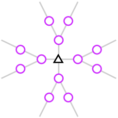
With the advent of modern database technology numerous large scale network data-sets have been made available. This development has triggered a surge of activity in studies of statistical network properties ba:rev ; mejn:rev ; doromen:book . The underlying idea of these studies is that the network structure (the way the networks differ from completely random networks) contain some information of the function, both locally and globally, of the network. Hence a common theme in these works has been the development of structural measures to characterize network structure. In this paper we propose and evaluate a measure of a previously unstudied network structure—a special case of symmetry we call degree symmetry. In geometry an object is symmetrical if it is invariant to rotations, reflections, and so on. In networks, with no given geometrical embedding, these concepts have to be relaxed. Furthermore, we would like to have a continuous measure saying not only if a vertex is a local center of symmetry or not, but also how symmetric the vertex is. The aspect of symmetry we address is, roughly speaking, that if you look at the object (network in our case) in different ways from a symmetric vertex it still looks the same. We process of “looking” will in our case be walking along paths (non-self intersecting sequences of edges). Furthermore, since degree (number of neighbors) is commonly regarded as the most fundamental quantity relating a vertex to its function, we say two vertices “look the same” if they have the same degree. We will thus derive our measure by performing walks along all paths from a vertex and compare the sequence of degrees of the vertices along these paths. The situation we have in mind is depicted in Fig. 1—all paths from the central vertex have degree sequences starting with $(3,2,\cdots)$, thus the central vertex is highly degree symmetric.

The rest of the paper is organized as follows: First we give a detailed derivation of the degree-symmetry coefficient (in two different versions, appropriate for different needs). Then we evaluate these on example networks and a biochemical network. Finally we discuss the average degree symmetry of different classes of real-world networks.

II Derivation of the measure

We will consider the network represented by a graph $G=(V,E)$ of $N$ vertices, $V$, and $M$ edges, $E$. For a vertex $i$ to have high degree symmetry it has, as mentioned, to have many paths with the same sequence of degrees. We will use a cut-off $l$ for the pathlength and consider only paths of that length. The reason for this cutoff is threefold: First, in all (with possibly some curious exception) network processes, a vertex is more affected by its closest surroundings then vertices further away. Thus one would like to have a lower weight on the contribution from distant vertices. Second, the number of vertices $n$ steps away grows fast with the distance from $i$. For finite networks this means that the paths soon reach the periphery of the network where unwanted finite-size effects set in. Third, for computation speed, one benefit from a cutoff.

Figure 2: Illustrations of of concepts in the derivation of the degree symmetry coefficient. (a) illustrates the branching number. Consider paths of length three out from $i$. The branching number of the path $(i,j)$ is five (there are five paths from $i$ of length three that goes through $j$). The branching number at $j^{\prime}$ is two. (b) shows the set $\Delta(P,i)$, where $P$ is the path $(i,j,j^{\prime})$.

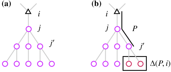
Assume there are $p$ paths of length $l$ from a vertex $i$. We then denote the degree sequences of these paths

$$Q_{l}(i) = \Big{\{}[k(v^{1}_{1,i,l}),\cdots,k(v^{l}_{1,i,l})],$$

$$\vdots$$

$$,[k(v^{1}_{p,i,l}),\cdots,k(v^{l}_{p,i,l})]\Big{\}},$$

where $k(v)$ denotes the degree of a vertex $v$ and $v^{j}_{m,i,l}$ is the $j$’th vertex of along the $m$’th path of length $l$ leading out from $i$. Then if there are unexpectedly many vertices at the same ($j$-) index in the sequence with the same degree, the vertex $i$ is a local center of degree symmetry. A rough symmetry measure would thus be to count the fraction of index-pairs with the same degree, i.e.

$$\frac{\tilde{s}_{l}(i)}{\Lambda}=\sum_{0\leq n<n^{\prime}\leq p}\sum_{j=1}^{l}\delta\big{(}k(v^{j}_{n,i,l}),k(v^{j}_{n^{\prime},i,l})\big{)},$$ (2)

where

$$\Lambda=(l-1)\>\dbinom{p}{2}\mbox{~{}~{}and~{}~{}}\delta(x,y)=\left\{\begin{array}[]{cl}1&\mbox{if $x=y$}\\ 0&\mbox{if $x\neq y$}\end{array}\right..$$ (3)

This measure is very crude and lack many desired statistical features. For example, all paths that go via a particular neighbor of $i$ will give a contribution to the sum. In practice this means that vertices with a high degree vertex rather far from itself (but closer that $l$) will trivially have a high $\tilde{s}_{l}(i)/\Lambda$. A first step would thus be to omit the contribution of vertices occurring in many sequences of $Q_{l}(i)$ at a specific index. I.e., for all $l^{\prime}\in(0,l)$ one wants to exclude the terms

$$\sum_{n,n^{\prime}}\delta\big{(}k(v^{1}_{n,i,l}),k(v^{1}_{n^{\prime},i,l})\big{)},$$ (4)

where $n$ and $n^{\prime}$ are indices of paths that are identical the first $l^{\prime}$ steps, from Eq. (2). Let $S_{l}(i)$ denote the number of such terms.

To calculate $S_{l}(i)$ consider a path $P=(i,\cdots,j)$ of length $l^{\prime}<l$. Let $b_{l}(P,i)$ be the number of paths from $i$ of length $l$ that start with the path $P$. We call $b_{l}(P,i)$ the branching number of $P$, see Fig. 2(a). All pairs of paths starting with $P$ will contribute to $\tilde{s}_{l}(i)$ a distance $l^{\prime}$ from $i$ (since they all pass through $j$). Let $\Delta(P,i)$ be the set of neighbors to $j$ that is not on the path $P$ from $i$ to $j$, see Fig. 2(b). (The number of elements in $\Delta(P,i)$ is thus $k_{j}-1$.) This situation gives a contribution

$$S_{l}(P,i)=\dbinom{b_{l}(P,i)}{2}+\sum_{j\in\Delta(P,i)}S_{l}((P,j),i)$$ (5)

from vertices of indices in the interval $[l^{\prime},l]$ of $Q_{l}(i)$ to $\tilde{s}_{l}(i)$, where $(P,j^{\prime})$ denotes the path $(i,\cdots,j,j^{\prime})$.

To further improve the measure one would like to, assuming some null-model, subtract the expected random contribution to $\tilde{s}_{l}(i)/\Lambda$. If this can be achieved one would have a symmetry coefficient $s_{l}(i)$ that is zero when the symmetry is what can be expected from the null-model, larger if $i$ is a center of unexpectedly high symmetry, and less than zero if $i$ is degree anti-symmetric. A final symmetry coefficient could thus be written

$$s_{l}(i)=\frac{\tilde{s}_{l}(i)-S_{l}(i)}{\Lambda-S_{l}(i)}-\nu,\mbox{~{}~{} provided $\Lambda>S_{l}(i)$}$$ (6)

where $\nu$ is the expected value of $(\tilde{s}_{l}(i)-S_{l}(i))/(\Lambda-S_{l}(i))$ in a null-model. $\Lambda=S_{l}(i)$ can only happen if there is one or no path of length $l$. In both these cases the degree-symmetry concept makes no sense so, if $\Lambda=S_{l}(i)\in\{0,1\}$, we set $s_{l}(i)=0$. The null-model we assume is random constrained on the degree distribution of the network. I.e., given the fraction $p_{k}$ of $k$-degree vertices the network is as random as possible. As it turns out $\nu$ is tricky to calculate analytically. There are two ways to proceed—either one calculates an approximative $\nu$ or one obtains $\nu$ via averaging $(\tilde{s}_{l}(i)-S_{l}(i))/(\Lambda-S_{l}(i))$ over realizations of the null-model. Except being more accurate, the latter approach has the advantage of giving an error estimate of $s_{l}(i)$—one can by specifying a p-value define significantly symmetric, or anti-symmetric, vertices. We will use both approaches: The approximative method for analyzing example networks and the numerical method for analyzing real-world data.

We obtain an approximative value of $\nu$, $\nu^{\mathrm{app.}}$, by assuming $\nu$ is approximately equal to the probability that a pair of vertices, reached by walking along paths, is the same. Note that, since there are $k$ ways into a degree-$k$ vertex, when following a path the probability to reach a degree-$k$ vertex is

$$\frac{kp_{k}}{\sum_{k^{\prime}}k^{\prime}p_{k^{\prime}}}=\frac{kp_{k}}{\langle k\rangle}.$$ (7)

Thus the probability $\nu^{\mathrm{app.}}$ that two vertices of the same degree is reached by following different paths is

$$\nu^{\mathrm{app.}}=\sum_{k}p_{k}\left(\frac{kp_{k}}{\langle k\rangle}\right)^{2}=\frac{1}{\langle k\rangle^{2}}\sum_{k}k^{2}p_{k}^{3}.$$ (8)

One reason this approach is not exact is that the number of terms in the expression for $\tilde{s}_{l}(i)$ increases with the degree of the $j$ in $\Delta(P,i)$ of Eq. (5). There are other higher-order effects to related to other correlations between the path structure and the degree of the vertices.

To summarize we have two measures of local vertex symmetry, one approximative:

$$s^{\mathrm{app.}}_{l}(i)=\frac{\tilde{s}_{l}(i)-S_{l}(i)}{\Lambda-S_{l}(i)}-\frac{1}{\langle k\rangle^{2}}\sum_{k}k^{2}p_{k}^{3},$$ (9)

and one based one Monte Carlo sampling

$$s^{\mathrm{MC}}_{l}(i)=\frac{\tilde{s}_{l}(i)-S_{l}(i)}{\Lambda-S_{l}(i)}-\left\langle\frac{\tilde{s}_{l}(i)-S_{l}(i)}{\Lambda-S_{l}(i)}\right\rangle.$$ (10)

The sampling is conveniently done by random rewiring the edges of the original network roberts:mcmc .

III Algorithm

The heart of algorithm, as suggested in the previous section, is a depth-first search with depth $l$. When the returning along the traced out paths the branching number can be calculated recursively through

$$b_{l}(P,i)=\left\{\begin{array}[]{ll}1&\mbox{if $P$ has length $l$}\\ \sum_{j^{\prime}\in\Delta((P,j^{\prime}),i)}b_{l}((P,j^{\prime}),i)&\mbox{otherwise}\end{array}\right..$$ (11)

$S_{l}(P_{i})$ can be calculated simultaneously using Eq. (5). A slight complication is that the same vertex may appear in different branches of the depth first search while calculating $b$ and $\tilde{s}$. For small cut-off values this is easy to handle: For $l=2$ it does not affect the calculation at all. For $l=3$ one would only have to keep different depths (of Eqs. (5) and (11)) separate. For the calculation of $\tilde{s}_{l}(i)$ the terms of $Q_{l}(i)$ has to be stored. Since the number of paths $p$ grows fast with $l$, this can be quite a constraint for a large $l$. Luckily it suffices to store a histogram $h(l^{\prime},k)$ counting the number of vertices of degree $k$ at position $l^{\prime}$ of the paths $Q_{l}(i)$. $p$ (and thus $\Lambda$) can be calculated as the number of time the depth $l$ of the depth first search is reached. The running time of the algorithm is $O(p)$. A mean field approximation for networks with few triangles gives $O(p)\approx O(\langle k\rangle^{l})$.

IV Extensions and considerations

The method outlined above can quite straightforwardly be extended to network with directed edges, distinct types of edges or (integer) edge weights.

Imagine a network with $z$ different edge sets $E_{1},\cdots,E_{z}$. Such networks frequently occur in cellular biochemistry—e.g. protein interaction networks where different types of protein interaction can be recorded hh:pfp , or gene regulation networks where the edges can be activating or inhibitory. One sensible way to extend the above procedure is to use the union of the edges as your graph but to say two pairs of vertices in $Q_{l}(i)$ are identical if their degrees with respect to all of the networks are the same. To formalize this $Q_{l}(i)$ would be generalized to

$$Q_{l}(i) = \Big{\{}[\mathbf{k}(v^{1}_{1,i,l}),\cdots,\mathbf{k}(v^{l}_{1,i,l})],$$

$$\vdots$$

$$,[\mathbf{k}(v^{1}_{p,i,l}),\cdots,\mathbf{k}(v^{l}_{p,i,l})]\Big{\}},$$

where $\mathbf{k}(v)$ is a vector with $v$’s degrees with respect to the different edge-types. and the $\delta$-function of Eq. (4) would be one if the arguments are equal at all their indices, and zero otherwise. The $\nu^{\mathrm{app.}}$ has to be redefined too:

$$\nu^{\mathrm{app.}}=\frac{1}{\langle k\rangle^{2}}\sum_{k^{\prime},k^{\prime\prime}}k^{\prime}p_{k^{\prime}}\,k^{\prime\prime}p_{k^{\prime\prime}}\prod_{i=1}^{z}\sum_{j=1}^{z}p_{i}(k_{j}|k^{\prime})p_{i}(k_{j}|k^{\prime\prime}),$$ (13)

where $p_{i}(k|k^{\prime})$ is the conditional probability that a vertex has degree $k$ with respect to edge set $E_{i}$ given that its degree in the union network is $k^{\prime}$. The case of a directed network can be treated similarly—one consider paths following edges in both directions but a vertex pair gives a contribution to $\tilde{s}$ only if both the in- and out-degrees are the same.

The approach of Sect. III can straightforwardly be applied to networks where multiple edges are allowed. Since multiple edges can be used to model weighted graphs mejn:wei the generalization to weighted graphs (at least where edge-weights represent the probability of following an edge) is simple. The other aspect of multigraphs, self-edges, is trivially dealt with—by the requirement that a paths should not intersect themselves a self-edge will never be followed and can thus be omitted already when the graph is constructed.

The overlap required for a vertex pair to be considered equal in the calculation of the symmetry coefficient is rather strict. Sometimes one would like to treat two paths as similar even if their degrees differs slightly. Particularly, this applies to broad degree distributions. The functional difference between degree-2 and degree-3 vertices may be significant; but whether a vertex has degree 1002 or 1003 probably does not matter. To achieve such a relaxation one can construct a integer sequence $K_{1}<K_{2}<\cdots$ and let

$$\delta(k,k^{\prime})=\left\{\begin{array}[]{cl}1&\mbox{if $K_{i}\leq k,k^{\prime}<K_{i+1}$ for some $i$}\\ 0&\mbox{otherwise}\end{array}\right..$$ (14)

I.e., one construct a series of equivalence classes of vertices. For a power-law, or similarly broad, degree distributions one can let $K_{i+1}-K_{i}$ increase exponentially with $i$. In this case one also has to modify the definition of $\nu^{\mathrm{app.}}$

$$\nu^{\mathrm{app.}}=\frac{1}{\langle k\rangle^{2}}\sum_{i}\left(\sum_{K_{i}\leq k<K_{i+1}}p_{k}\right)\left(\sum_{K_{i}\leq k<K_{i+1}}kp_{k}\right)^{2}.$$ (15)

Figure 3: Degree symmetries of small example networks. (a) is consistent with the example Fig. 1(a). (b) is an example of a graph with only positive degree symmetries. (c) shows a graph with only negative degree symmetries. The cut-off length $l=2$ is used.

V Degree symmetries of example networks

In this section we evaluate the measure for example networks and real-world networks. We will use the smallest non-trivial cut-off $l=2$ throughout this section. Most conclusions hold for $l=3$ or $4$.

V.1 Small test graphs

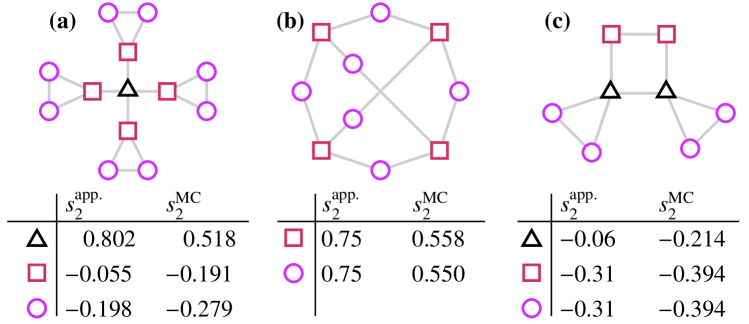
To get a feeling for the $s_{l}$ measure we start by considering a few small test networks, see Fig. 3. In Fig. 3(a) we display a network with the same degree symmetry, with respect to the central vertex (triangle), as Fig. 1. As expected the central vertex has a strong degree symmetry coefficient. To carry through the calculation of Eq. (9) once we obtain the degree distribution $p_{2}=8/13$, $p_{3}=4/13$ and $p_{4}=1/13$ giving $\nu^{\mathrm{app.}}=165/832\approx 0.198$. All length-2 paths out from the central vertex have the degree sequence $(3,2)$ so $\tilde{s}_{2}(\triangle)=4$, $S_{2}(\triangle)=4$ and $\Lambda=28$ giving $s_{2}^{\mathrm{app.}}(\triangle)=667/832\approx 0.802$. The degree-3 vertices (squares) have two degree sequences of their outgoing paths $(4,3)$ and $(2,2)$, whereas paths from degree-2 vertices (triangles) have degree sequences $(3,4)$ and $(2,3)$. This difference is larger than expected from the null model (random networks with eight degree-2 vertices, four degree-3 vertices and one degree-4 vertex), thus the negative $s_{2}$ values for these vertices.

In Fig. 3(b) we show a graph where all vertices have positive degree-symmetry coefficient. Paths from degree-2 vertices have only the degree sequence $(3,2)$ and paths from degree-3 vertices have only the degree sequence $(2,3)$. Thus, for every vertex, the view of degrees along the path out to the rest of the network is the same no matter which direction one looks in from that vertex. A radically different view is seen in Fig. 3(c). In this case the vertices have three distinct positions in the network. The vertices marked with squares have degree two and four outgoing paths of degree sequences $(2,4)$, $(4,4)$, $(4,2)$ and $(4,2)$. The circles, despite their different network position (as being part of triangles), have the same set of degree sequences for their paths of length two. The degree-3 vertices have six length-2 paths: three having the degree sequence $(2,2)$, three having degree sequence $(4,2)$. It is easy to convince oneself that this close to as dissimilar a network with four degree-2 and two degree-4 vertices can be. Consequently all vertices have negative degree-symmetry indices. It is worth pointing out that the Fig. 3(c) possesses other symmetries than degree-symmetry. The layout has, for example, reflexive symmetry along a vertical axis. We emphasize that such symmetries would need to be captured by other measures.

V.2 Regular networks

If all vertices have the same degree a network is called regular janson . Then by definition all paths are known to fully overlap. This trivial overlap should be canceled in our symmetry measure so $s_{l}(i)=0$ for all $l$ and $i$. Since $S_{l}(i)$ is the number of terms in $\tilde{s}_{l}(i)$ and all these terms are one we have $S_{l}(i)=\tilde{s}_{l}(i)=\Lambda$. Furthermore, $\nu^{\mathrm{app.}}=1$ which gives $s_{l}(i)$ for all vertices and cut-off lengths.

V.3 Random graphs

Figure 4: The average approximative symmetry coefficient for $l=3$ and random graphs with $M=2N$. The line is a fit to a power-law decay form ($0.124+0.435N^{-1.02}$, to be exact).

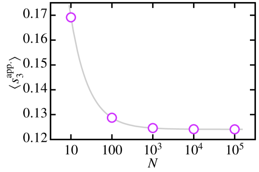
Next we evaluate the average approximative symmetry coefficient $\langle s^{\mathrm{app.}}\rangle$ for random graphs janson —graphs obtained by successively adding $M$ edges between $N$ vertices with the restriction that no multiple edge, or self-edge, may occur. Such networks have no correlations at all and can serve as a reference point for neutrality mejn:rev . Ideally we would like such networks to, on average, have a degree-symmetry coefficient of zero. As seen in Fig. 4 $\langle s^{\mathrm{app.}}_{l}\rangle$ converge to a small but positive value. The decay is roughly inversely proportional to $N$—the same scaling as the fraction of triangles in the network—which suggests that the presence of triangles, and perhaps other short-cycles, is an important source of finite size effects of $s^{\mathrm{app.}}_{l}$. We conclude that the Monte Carlo sampling measure $s^{\mathrm{MC}}_{l}$ (or a more elaborate measure) is needed if one wants to compare different networks. If, on the other hand, one aims to compare different vertices of the same network the faster $s^{\mathrm{app.}}_{l}(i)$ calculation is sufficient. This is not an uncommon situation in the design of network measures. Another example of this where neutrality is non-zero in the large-$N$ limit is modularity, measuring how good a subgraphs that are densely connected within but not between each other gui:mod .

VI Degree symmetries of real networks

In this section we apply our measures to real-world networks. First we take a look at the symmetry coefficients of specific vertices in the metabolic network of humans, then we look at the average symmetry coefficients of various classes of networks.

VI.1 Human metabolic networks

Figure 5: The 2-neighborhood of spermine—a vertex with high degree-symmetry—(a), and C04850—a vertex with low degree symmetry—(b), in the human metabolic network. The symbols indicate the equivalence classes defined by exponentially growing intervals. Filled circles have degree two, unfilled circles have degree four or five, a vertex symbolized by an $n$-gon have degree in the interval $[2^{n},2^{n+1})$. In case the chemical names are overly long the KEGG codes are given (“C” and five digits): C07282 represents eIF5A-precursor-deoxyhypusine, C04850 represents 1,3-$\beta$-D-galactosyl-($\alpha$-1,4-L-fucosyl)-N-acetyl-D-glucosaminyl-R, C04556 represents 4-amino-2-methyl-5-phosphomethylpyrimidine, C04467 represents $\alpha$-L-fucosyl-1,2-$\beta$-D-galactosyl-R and C01311 represents 1,4-$\beta$-D-galactosyl-($\alpha$-1,3-L-fucosyl)-N-acetyl-D-glucosaminyl-R.

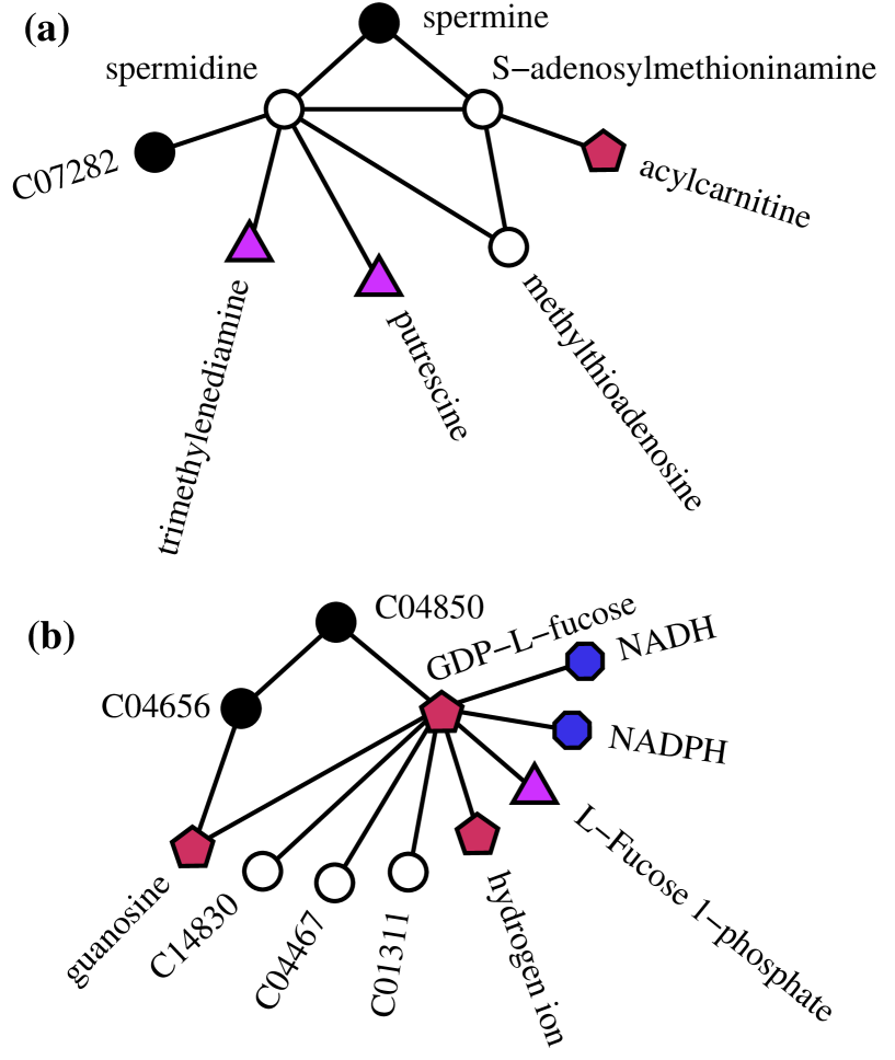
An important use of statistical graph theory is to characterize chemical reaction networks. Of many possible network representations zhao:meta we let vertices be chemical substances, and for all reactions of an organism we link substrates with products. For example, the hypothetical reaction $\mathrm{A}+\mathrm{B}\longleftrightarrow\mathrm{C}+\mathrm{D}$ would contribute with the edges $(\mathrm{A},\mathrm{C})$, $(\mathrm{A},\mathrm{D})$ and $(\mathrm{B},\mathrm{C})$, $(\mathrm{B},\mathrm{D})$ to the metabolic network. The data is derived from the KEGG database (http://www.genome.jp/), and described in detail in Ref. our:bio . Since the degree distributions of metabolic networks are highly skewed jeong:meta we use a exponentially increasing set of intervals as equivalence classes (as discussed in the connect of Eq. (14)): $K_{n}=2^{n}$.

It has been argued that degree is strongly related to the function of the chemical substance jeong:meta ; gui:meta . This means that the degree symmetry potentially can give additional information about the function of the vertices. For the human metabolic network, and $l=2$, roughly half of the vertices have a p-value of less than 5% (i.e., in the null-model sampling of the calculation of $s_{2}^{\mathrm{MC}}$, less than 5% or more than 95% of the values of

$$\frac{\tilde{s}_{l}(i)-S_{l}(i)}{\Lambda-S_{l}(i)}$$ (16)

are smaller than the value of the real network). In Fig. 5(a) we show the 2-neighborhood of one vertex with significantly higher $s_{2}^{\mathrm{MC}}$ than expected; Fig. 5(b) depict the 2-neighborhood of a vertex with significantly higher $s_{2}^{\mathrm{MC}}$. The reason these particular vertices are used as examples is that their 2-neighborhoods are of appropriate sizes, neither too big, nor too small, to be displayed and described. Spermine, Fig. 5(a), is a substance with high degree-symmetry—$s_{2}^{\mathrm{MC}}=0.89\pm 0.02$. Both its neighbors are in the same degree-equivalence class of vertices with degree four to seven. Of vertices two steps away from spermine there is also a significant overlap with two (out of four) neighbors to the neighbor spermidine being in the equivalence class defined by degrees in the interval $[8,16)$; whereas two vertices are in the equivalence class of degrees in $[4,8)$. The three paths from spermine via S-adenosylmethioninamine also contribute to the overlap in the two steps from spermine as two vertices (methylthioadenosine and spermindine) have degrees in the same equivalence class. The neighborhood of C04850, seen in Fig. 5(b), is visually less balanced and also having a negative degree-symmetry—$s_{2}^{\mathrm{MC}}=-0.11\pm 0.01$. We note that there are some vertex pairs in the second neighborhood whose degree-classes overlap, but apparently this is not enough to make the symmetry coefficient non-negative.

VI.2 Average symmetry values

Table 1: The network sizes $N$ and $M$ and the average numerical degree-symmetry coefficient $s_{2}^{\mathrm{MC}}$ of real-world networks. In the interstate network the vertices are American interstate highway junctions and two junctions are connected if there is a road with no junction in between. In the street networks the vertices are Swedish city-street segments connected if they share a junction. In the airport network (obtained from http://vlado.fmf.uni-lj.si/pub/networks/pajek/data/gphs.htm) the vertices are American airports and edges represent a regular, non-stop route. In the citation networks the vertices are papers and two papers are connected if they one cites the other. The “scientometrics” network consists of papers from the journal Scientometrics. The “small-world” network are all papers citing Ref. milg:1 or having the phrase “small world” in the title. (The citation networks were obtained from http://vlado.fmf.uni-lj.si/pub/networks/data/cite/. These networks are the result of searches in the WebofScience used with the permission of ISI Philadelphia.) The board of directors and Ajou student networks are derived from one-mode projections of affiliation networks (where edges goes from persons to corporate boards and university classes respectively). The Ajou student network is averaged over graphs of 16 semesters. One edge represent two students taking at least three classes together that semester. The high school networks are gathered from questionnaires—an edge means that two persons have listed each other as acquaintances. It is averaged over 84 individual schools. In the electronic communication networks one edge represent that at least one of the vertices has contacted the other over some electronic medium. The food webs are networks of water-living species and an edge means that one species prey on the other. For the protein networks an edge means that two proteins interact (the two graphs correspond to two different types of experiments determining the interaction edges). The metabolic networks consist of chemical substances and edges are constructed as described in Sect. VI.1. Values for animal metabolism is averaged over six networks, fungi metabolism is averaged over two, and bacteria metabolism is averaged over 96 networks.

network		Ref.	$N$	$M$	$s_{2}^{\mathrm{MC}}$
geographical networks	interstate highways		935	1315	$0.016\pm 0.003$
	streets, Stockholm	rosv:city	3325	5100	$0.014\pm 0.003$
	streets, Malmö	rosv:city	1868	3026	$0.020\pm 0.003$
	streets, Göteborg	rosv:city	1258	1516	$0.026\pm 0.003$
	airport		332	2126	$-0.0573\pm 0.0002$
citation networks	scientometrics		2728	10398	$0.015\pm 0.020$
	small-world		233	994	$0.007\pm 0.002$
one-mode projections of	board of directors	davis	6193	43074	$0.175\pm 0.004$
affiliation networks	Ajou University students	our:ajou2	$7285\pm 128$	$75898\pm 6566$	$0.13\pm 0.01$
acquaintance networks	high school friendship	addh	$571\pm 43$	$1104\pm 60$	$0.020\pm 0.002$
electronic communication networks	e-mail	eckmann:dialog	3186	31856	$-0.01\pm 0.01$
	Internet community	pok	28295	115335	$0.01898\pm 0.0001$
food webs	Little Rock lake	martinez:rock	92	960	$0.042\pm 0.001$
	Ythan estuary	ythan1	134	593	$0.027\pm 0.002$
neural network	C. elegans	cenn:brenner	280	1973	$0.0839\pm 0.0001$
biochemical networks	S. cervisiae protein	pagel:mips ; hh:pfp	4580	7434	$0.0205\pm 0.0001$
	S. cervisiae genetic	pagel:mips ; hh:pfp	4580	5129	$0.0996\pm 0.0001$
	animal metabolism	our:bio	$1621\pm 123$	$4662\pm 473$	$0.02\pm 0.01$
	plant metabolism, A. thaliana	our:bio	1561	4302	$0.0133\pm 0.0003$
	fungi metabolism	our:bio	$1281\pm 97$	$3654\pm 289$	$0.03\pm 0.02$
	bacteria metabolism	our:bio	$1070\pm 35$	$2776\pm 109$	$0.018\pm 0.002$

So far we have discussed degree symmetries of vertices. In this section we average $s_{l}$ over $V$ to obtain a graph-wide measure for degree symmetry. In Table 1 we display values of $s_{2}^{\mathrm{MC}}$ for a number of different network types. Some of these have highly skewed degree distributions. For these, the exponentially increasing degree equivalence classes of Sect. VI.1 are appropriate. Since we intend to compare all networks we use the same equivalence classes for all networks. The first observation is that almost all networks have a positive average symmetry coefficient. The only clear exception is the airport network. This means that if you start a two-leg airplane trip at a particular airport, choosing between two random itineraries (without caring about the frequency of flights), then the probability of the airports along these itineraries being different in number of connections is smaller than in a random network. The strongest degree-symmetries are found in one-mode projections of social affiliation networks. Note that the other social networks, derived from questionnaires and electronic communication does not have such strong symmetry coefficients. In one-mode projections high-degree vertices are known to have strong tendency to attach to other high-degree vertices, and low-degree vertices to attach to other low-degree-vertices—so called assortative mixing mejn:assmix . If this property is strong there will be regions of vertices with high degree and other regions with low-degree vertices. The paths within these regions would also have similar degree sequences. Thus high assortative mixing can be related to high degree symmetry, the first causing the second or vice versa. They are, of course, not equivalent—e.g., the example network with all vertices having positive symmetry coefficients (Fig. 3(b)) is maximally disassortatively mixed (in the sense of Ref. mejn:assmix ). Where the weak symmetry coefficients of other networks come from is outside the scope of this investigation. One possible explanation would be that functional units alon might often be degree-symmetric centers.

VII Summary and conclusions

We have derived a measure for a specific notion of symmetry in networks—the property that the paths out from a vertex have overlapping degree sequences. The measure is designed so that random networks, conditioned only to have the same set of degrees as the original network, have the value zero. We propose two versions of the symmetry coefficient, the first being approximately zero for random networks, the second requiring a randomization procedure (and thus longer simulation time) but being more accurately zero for random networks. The measure was evaluated on example graphs. We show that they are able to detect vertices in degree-symmetric, and potentially functionally meaningful positions in the human metabolic network. The average degree-symmetry of various networks were also investigated. We found almost all networks having a weakly positive degree coefficient. The exceptions being the network of American airports and their interconnections (having a negative degree-symmetry coefficient) and one-mode projections of social affiliation networks (having rather strongly positive values). Our measure is not the first to be based on a the properties of paths going out from a vertex. For example people have been using path counts for assessing the functional similarity of pairs of vertices blondel:sim ; simrank ; our:sim . In social network studies such measures are commonly called “ego-centric” wf .

Symmetry concepts have been successfully utilized in many field of physics. We believe degree symmetry, and other classes of network symmetries, will be a fruitful direction of future network studies. Degree symmetry is in particular, we believe, an important concept for networks where degree is strongly related to the function of the vertex. Two open questions from this study is what causes the rather ubiquitous weakly positive degree symmetries, and what process in the airline decision making that causes the negative average symmetry coefficient of the airline network.