Multipole (E1, M1, E2, M2, E3, M3) transition wavelengths and rates between $3l^{-1}5l^{\prime}$ excited and ground states in nickel-like ions

Abstract

A relativistic many-body method is developed to calculate energy and transition rates for multipole transitions in many-electron ions. This method is based on relativistic many-body perturbation theory (RMBPT), agrees with MCDF calculations in lowest-order, includes all second-order correlation corrections and includes corrections from negative energy states. Reduced matrix elements, oscillator strengths, and transition rates are calculated for electric-multipole (dipole (E1), quadrupole (E2), and octupole (E3)) and magnetic-multipole (dipole (M1), quadrupole (M2), and octupole (M3)) transitions between $3l^{-1}5l^{\prime}$ excited and ground states in Ni-like ions with nuclear charges ranging from $Z$ = 30 to 100. The calculations start from a $1s^{2}2s^{2}2p^{6}3s^{2}3p^{6}3d^{10}$ Dirac-Fock potential. First-order perturbation theory is used to obtain intermediate-coupling coefficients, and second-order RMBPT is used to determine the matrix elements. A detailed discussion of the various contributions to the dipole matrix elements and energy levels is given for nickellike tungsten ($Z$ = 74). The contributions from negative-energy states are included in the second-order E1, M1, E2 M2, E3, and M3 matrix elements. The resulting transition energies and transition rates are compared with experimental values and with results from other recent calculations. These atomic data are important in modeling of M-shell radiation spectra of heavy ions generated in electron beam ion trap experiments and in M-shell diagnostics of plasmas.

I Introduction

The Ni-isoelectronic sequence has been studied extensively in connection with x-ray lasers  Smith et al. (2005); Keenan et al. (2005); Kawachi et al. (2004); Janulewicz et al. (2003); Mocek et al. (2003); Norreys et al. (1993); Scofield and MacGowa (1992); Chen and Osterheld (1995); Li et al. (1998); Daido et al. (1999); Nilsen et al. (1999). Recently, an investigation into the use of atomic databases in simulation of Ni-like gadolinium x-ray laser was presented by King et al. in Ref. King et al. (2004). Measurements of $3d-5f$ and $3d-6f$ transition energies in Ni-like ions (Ag¹⁹⁺, Sn²²⁺, Pr³¹⁺, Gd³⁶⁺, Yb⁴²⁺, Ta⁴⁵⁺, Ir⁴⁹⁺, Th⁶²⁺, and , U⁶⁴⁺) were reported by Elliott et al. in Ref. Elliott et al. (1994). Additional measurements of the $3d_{5/2}-6f_{7/2}$ transition energies in Ni-like Tm⁴¹⁺, Hf⁴⁴⁺, Re⁴⁷⁺, Pb⁵⁴⁺, and Th⁶²⁺ were carried out by Beiersdorfer in Ref. Beiersdorfer et al. (1992). Recently, the x-ray spectral measurements of the line emission of $n$ = 3–4, 3–5, 3–6, and 3–7 transitions in Ni- to Kr-like Au ions in electron beam trap (EBIT) plasma were reported by May et al. in Ref. May et al. (2003). X-ray spectra of Ni-like W including 3-4, 5, and 6 transitions recorded by a broadband microcalorimeter, were analyzed in Ref. Shlyaptseva et al. (2004); Neill et al. (2004). A detailed analysis of 3-4 and 3-5 transitions in the x-ray spectrum by laser produced plasmas of Ni-like highly-charged ions was presented by Doron et al. Doron et al. (1998) (Ba²⁸⁺), by Zigler et al. Zigler et al. (1994) (La²⁹⁺ and Pr³¹⁺), by Doron et al. Doron et al. (2000) (Ce³⁰⁺). Studies of Ni-like ions (Gd³⁶⁺, W⁴⁶⁺ have also been carried out on tokamaks  S. von Goeler et al. (1988); Neu et al. (1997).

Various computer codes were employed to calculate transitions in Ni-like ions. In particular, ab-initio calculations were performed in Ref. Doron et al. (1998) using the relac relativistic computer code to identify $3d-nf$ ($n$=4 to 8) transitions of Ni-like Ba. Atomic structure calculations for highly ionized tungsten (Co-like W⁴⁷⁺ to Rb-like W³⁷⁺) were done by Fournier Fournier (1998) with using the graphical angular momentum coupling code ANGULAR and the fully relativistic parametric potential code RELAC. The Hebrew University Lawrence Livermore Atomic Code hullac is also based on a relativistic model potential Klapisch et al. (1977). Ab-initio calculations with the hullac relativistic code was used for detailed analysis of spectral lines by by Zigler et al. Zigler et al. (1994) and by May et al. in Ref. May et al. (2003). Zhang et al. Zhang et al. (1991), using the Dirac-Fock-Slater (DFS) code evaluated excitation energies and oscillator strengths of 3-4 and 3-5 transitions for the 33 Ni-like ions with 60$\leq Z\geq$92. The multiconfiguration Dirac=Fock calculations of the $3d_{3/2}-5f_{5/2}$, $3d_{5/2}-5f_{7/2}$, $3d_{3/2}-6f_{5/2}$, and $3d_{5/2}-6f_{7/2}$ transitions were reported by Elliot et al. in Ref. Elliott et al. (1994). The wavelengths and transition rates for $3l-nl^{\prime}$ electric-dipole transitions in Ni-like xenon are presented by Skobelev et al. in Ref. Skobelev et al. (199). Results were obtained by three methods: the relativistic Hartree-Fock (HFR) self-consistent-field method (Cowan code), multiconfiguration Dirac=-Fock (MCDH) method (Grant code), and the hullac code. The contribution of lots of weak correlation on transition wavelengths and probabilities by including partly single and double excitation from the $3l$ inner-shells into the $4l$ and $5l$ orbital layers of highly-charged Ni-like ions were discussed by Dong et al. in Ref. Dong et al. (2003). Energy levels, transition probabilities, and electron impact excitation for possible x-ray line emissions of Ni-like tantalum ions were recently calculated by Zhong et al. in Ref. Zhong et al. (2005).

The relative magnitudes of the electric-multipole (E1, E2, E3) and magnetic-multipole (M1, M2, M3) radiative decay rates calculated by the MCDF approach, were presented by Biémont Biémont (1997) for  lowest 17 levels of highly ionized nickel-like ions. Observation of electric-quadrupole (E2) and magnetic-octupole (M3) decay in the x-ray spectrum of highly charged Ni-like ions (Th⁶²⁺ and U⁶⁴⁺) were reported by Beiersdorfer et al. in Ref. Beiersdorfer et al. (1991). The lowest excited level in Ni-like ions, $3d^{9}4d\ ^{3}D_{3}$, decays only via an M3 decay. The radiative decay of this line was measured recently in Xe²⁶⁺, Cs²⁷⁺, and XBa²⁸⁺ by Träbert et al.  Träbert et al. (2005, 2006). Calculated values of transitions wavelengths and rates for Ni-like ions with 30$\leq Z\leq$100 presented in Ref. Träbert et al. (2005) were obtained by using Relativistic Many-Body Perturbation Theory (RMBPT) method. Reduced matrix elements, oscillator strengths, and transition rates into the ground state for all allowed and forbidden electric- and magnetic-dipole and electric- and magnetic-quadrupole transitions (E1, M1, E2, M2) in Ni-like ions were presented by Hamasha et al. in Ref. Hamasha et al. (2004). Relativistic many-body calculations of multipole (E1, M1, E2, M2, E3, M3) transition wavelengths and rates between $3l^{-1}4l^{\prime}$ excited and ground states in nickel-like ions were recently reported by Safronova et al. in Ref. Safronova et al. (2006).

In the present paper, RMBPT is used for systematic study of atomic characteristics of transitions in Ni=like ions in a broad range of the nuclear charge $Z$ = 3–100. Specifically, we determine energies of $3s^{2}3p^{6}3d^{9}5l(J)$, $3s^{2}3p^{5}3d^{10}5l(J)$, and $3s3p^{6}3d^{10}5l(J)$ states of Ni-like ions with nuclear charges $Z$=30-100. The calculations are carried out to second order in perturbation theory. We consider all possible $3l$ holes and $5l$ particles leading to the 67 odd-parity $3d^{-1}5p(J)$, $3d^{-1}5f(J)$, $3p^{-1}5s(J)$, $3p^{-1}5d(J)$, $3p^{-1}5g(J)$, $3s^{-1}5p(J)$, and $3s^{-1}5f(J)$ excited states and the 74 even-parity $3d^{-1}5s(J)$, $3d^{-1}5d(J)$, $3d^{-1}5g(J)$, $3p^{-1}5p(J)$, $3p^{-1}5f(J)$, $3s^{-1}5s(J)$, $3s^{-1}5d(J)$ and $3s^{-1}5g(J)$ excited states in Ni-like ions with $Z$=30 to 100.

RMBPT is also used to determine line strengths, oscillator strengths, and transition rates for all allowed and forbidden electric-multipole and magnetic-multipole (E1, E2, E3, M1, M2, M3) from $3s^{2}3p^{6}3d^{9}5l(J)$, $3s^{2}3p^{5}3d^{10}5l(J)$, and $3s3p^{6}3d^{10}5l(J)$ excited states into the ground state in Ni-like ions. Retarded E1, E2, and E3 matrix elements are evaluated in both length and velocity forms. A detailed discussion of the various contributions to the dipole matrix elements and energy levels is given for nickellike tungsten ($Z$ = 74), which plays an important role in tokamaks  S. von Goeler et al. (1988); Neu et al. (1997), electron beam ion traps  Neill et al. (2004); Hutton et al. (2003); Radtke et al. (2001), x-ray lasers  Elliott et al. (1995), and z-pinches  Shlyaptseva et al. (2004).

Figure 1: Mixing coefficients for the $3p5d\ ^{1,3}P_{1}$ levels as functions of $Z$

Figure 2: Energies ($E/(Z-21)^{2}$) in  cm^-1 for odd- and even-parity states in Ni-like ions as functions of $Z$

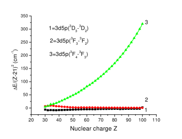
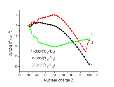
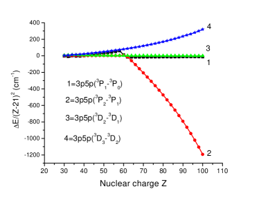
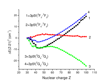
Figure 3: Energy splitting ($\Delta E/(Z-21)^{2}$) in  cm^-1 for terms of odd- and even-parity states with in Ni-like ions as function of $Z$

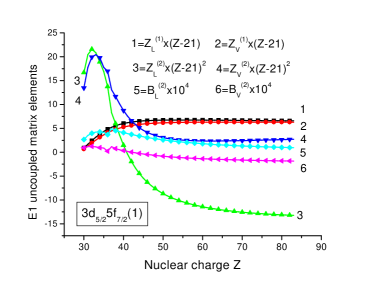
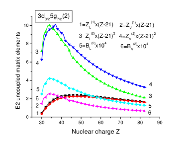
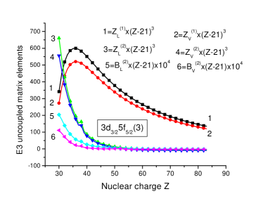
Figure 4: The first- and second-order Coulomb corrections ($Z^{(1)}$, $Z^{(2)}$), and second-order Breit-Coulomb corrections ($B^{(2)}$) for E1, E2, and E3 uncoupled matrix elements for transitions between excited and ground states calculated in length ($L$)and velocity ($V$) forms in Ni-like ions.

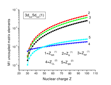
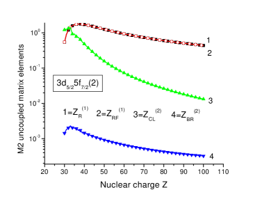
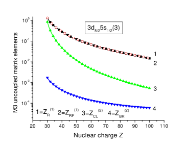
Figure 5: The first- and second-order corrections ($Z^{(1)}$, $Z^{(2)}$) for M1, M2 and M3 uncoupled matrix elements for transition between excited and ground states in Ni-like ions. The first-order ($Z^{(1)}$) matrix elements calculated in nonrelativistic ($Z^{(1)}_{\rm NR}$), relativistic frequency-independent($Z^{(1)}_{\rm R}$), and relativistic frequency-dependent ($Z^{(1)}_{\rm RF}$) approximations are presented. The second-order Coulomb ($Z^{(2)}_{\rm CL}$) and Breit-Coulomb corrections ($Z^{(2)}_{\rm BR}$)) are compared.

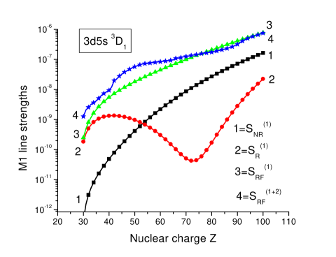
Figure 6: The total M1 line strengths ($S^{(1+2)}_{\rm RF}$) between the $3d5s\ ^{1}P_{1}$ and ground states in Ni-like ions as function of $Z$. The first-order ($S^{(1)}$) line strengths calculated in nonrelativistic ($S^{(1)}_{\rm NR}$), relativistic frequency-independent ($S^{(1)}_{\rm R}$), and relativistic frequency-dependent approximations ($S^{(1)}_{\rm RF}$) are presented.

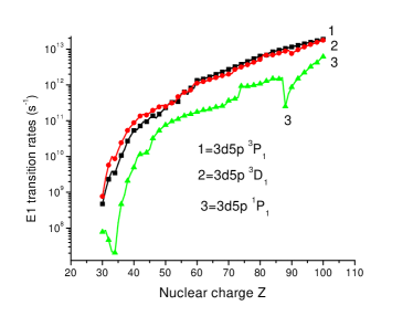
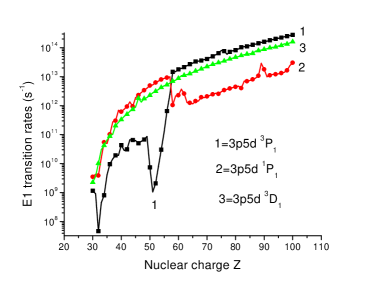
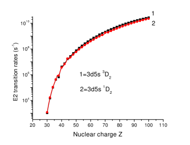
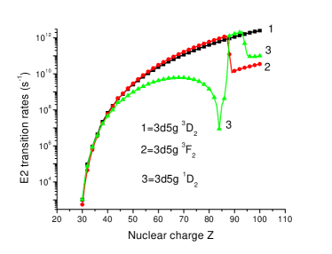
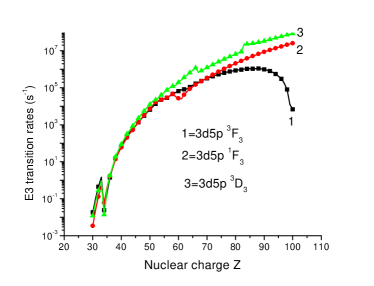
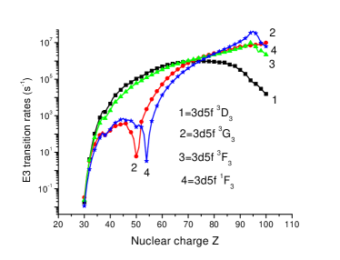
Figure 7: E1,E2, and E3 transition rates for transitions between the $3l5l^{\prime}$ states with $J$=1–3 and ground state in Ni-like ions as function of $Z$

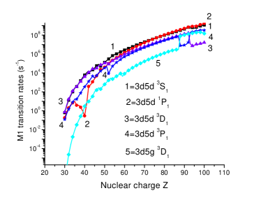
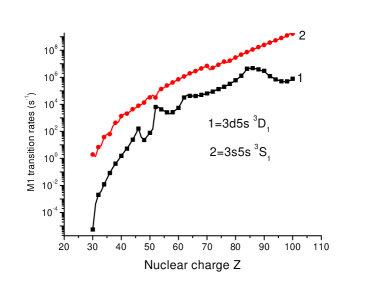
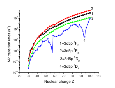
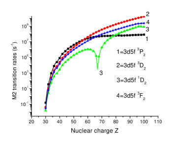
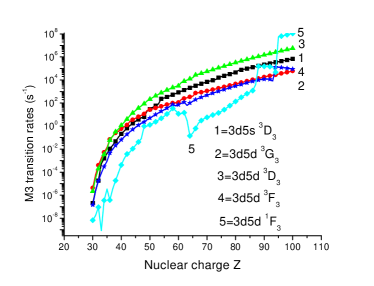
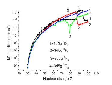
Figure 8: M1, M2, and M3 transition rates between the $3l5l^{\prime}$ states with $J$=1–3 and ground state in Ni-like ions as function of $Z$

II METHOD

Details of the RMBPT method were presented in Refs. Avgoustoglou et al. (1992); Safronova et al. (2000) for calculation of energies of hole-particle states, in Ref. Safronova et al. (1996) for calculation of energies of particle-particle states, in Ref. Safronova et al. (1999a) for calculation of radiative electric-dipole rates in two-particle states, and in Ref. Safronova et al. (2001); Hamasha et al. (2004) for calculation of radiative electric-dipole, electric-quadrupole, magnetic-dipole, and magnetic-quadrupole rates in Ne- and Ni-like systems. We will present here only the model space for Ni-like ions without repeating the detailed discussions given in Avgoustoglou et al. (1992); Safronova et al. (2000), Safronova et al. (1996),Safronova et al. (1999a), and Safronova et al. (2001); Hamasha et al. (2004). The calculations are carried out using sets of basis Dirac-Hartree-Fock (DHF) orbitals. The orbitals used in the present calculation are obtained as linear combinations of B-splines. These B-spline basis orbitals are determined using the method described in Ref. Johnson et al. (1988). We use 50 B-splines of order 10 for each single-particle angular momentum state and we include all orbitals with orbital angular momentum $l\leq 9$ in our basis set.

For atoms with one hole in closed shells and one electron above closed shells, the model space is formed from hole-particle states of the type $a_{v}^{+}a_{a}|0\rangle\,,$ where $|0\rangle$ is the closed-shell $1s_{1/2}^{2}2s_{1/2}^{2}2p_{1/2}^{2}2p_{3/2}^{4}3s_{1/2}^{2}3p_{1/2}^{2}3p_{3/2}^{4}3d_{3/2}^{4}3d_{3/2}^{6}$ ground state. The single-particle indices $v$ range over states in the valence shell and the single-hole indices $a$ range over the closed core. For our study of low-lying states $3l^{-1}4l^{\prime}$ states of Ni-like ions, values of $a$ are $3s_{1/2}$, $3p_{1/2}$, $3p_{3/2}$, $3d_{3/2}$, and $3d_{5/2}$,while values of $v$ are $5s_{1/2}$, $5p_{1/2}$, $5p_{3/2}$, $5d_{3/2}$, $5d_{5/2}$ $5f_{5/2}$, $5f_{7/2}$, $5g_{7/2}$, and $5g_{9/2}$. To obtain an orthonormal model states, we consider the coupled states $\Phi_{JM}(av)$ defined by

$$\Phi_{JM}(av) = \sqrt{(2J+1)}\sum_{m_{a}m_{v}}(-1)^{j_{v}-m_{v}}\left(\begin{array}[]{ccc}j_{v}&J&j_{a}\\ -m_{v}&M&m_{a}\end{array}\right)a_{vm_{v}}^{\dagger}a_{am_{a}}|0\rangle\,.$$ (3)

Combining the $n=3$ hole orbitals and the $n=4$ particle orbitals in nickel, we obtain 68 odd-parity states consisting of 5 $J=0$ states, 13 $J=1$ states, 16 $J=2$ states, 15 $J=3$ states, 11 $J=4$ states, six $J=5$ states, and two $J=6$ states. Additionally, there are 74 even-parity states consisting of 5 $J=0$ states, 13 $J=1$ states, 17 $J=2$ states, 16 $J=3$ states, 12 $J=4$ states, seven $J=5$ states, three $J=6$ states, and one $J=7$ state. The distribution of the 142 states in the model space is summarized in Table 1. In this table, we give both $jj$ and $LS$ designations for hole-particle states. Instead of using the $3l_{j}^{-1}5l^{\prime}_{j^{\prime}}$ or $3l^{-1}5l^{\prime}$ designations, we use simpler designations $3l_{j}5l^{\prime}_{j^{\prime}}$ or $3l5l^{\prime}$ in this table and in all following tables and the text below.

III Excitation energies

III.1 Example: Energy matrix for W⁴⁶⁺

In Table 2, we give various contributions to the second-order energies for the special case of Ni-like tungsten, $Z=74$. In this table, we show the one-body and two-body second-order Coulomb contributions to the energy matrix labeled $E^{(2)}_{1}$ and $E^{(2)}_{2}$, respectively. The corresponding Breit-Coulomb contributions are given in columns headed $B^{(2)}_{1}$ and $B^{(2)}_{2}$. The one-body second-order energy is obtained as a sum of the valence $E^{(2)}_{v}$ and hole $E^{(2)}_{a}$ energies with the latter being the dominant contribution. The values of $E^{(2)}_{1}$ and $B^{(2)}_{1}$ are non-zero only for diagonal matrix elements. Although there are 142 diagonal and 1636 non-diagonal matrix elements for $(3l_{j}5l^{\prime}_{j^{\prime}})\,(J)$ hole-particle states, we list only the part of odd-parity subset with $J$=1 in Table 2. It can be seen from the table that second-order Breit-Coulomb corrections are relatively large and, therefore, must be included in accurate calculations. The values of non-diagonal matrix elements given in columns headed $E^{(2)}_{2}$ and $B^{(2)}_{2}$ are comparable with values of diagonal two-body matrix elements. However, the values of one-body contributions, $E^{(2)}_{1}$ and $B^{(2)}_{1}$, are larger than the values of two-body contributions, $E^{(2)}_{2}$ and $B^{(2)}_{2}$, respectively. As a result, total second-order diagonal matrix elements are much larger than the non-diagonal matrix elements, which are shown in Table 3.

In Table 3, we present results for the zeroth-, first-, and second-order Coulomb contributions, $E^{(0)}$, $E^{(1)}$, and $E^{(2)}$, and the first- and second-order Breit-Coulomb corrections, $B_{hf}^{(1)}$ and $B^{(2)}$. It should be noted that corrections for the frequency-dependent Breit interaction Chen et al. (1993) are included in the first order only. The difference between the first-order Breit-Coulomb corrections calculated with and without frequency dependence is less than 1%. As one can see from Table 3, the ratio of non-diagonal and diagonal matrix elements is larger for the first-order contributions than for the second-order contributions. Another difference in the first- and second-order contributions is the symmetry properties: the first-order non-diagonal matrix elements are symmetric and the second-order non-diagonal matrix elements are not symmetric. The values of $E^{(2)}[a^{\prime}v^{\prime}(J),av(J)]$ and $E^{(2)}[av(J),a^{\prime}v^{\prime}(J)]$ matrix elements differ in some cases by a factor 2–3 and occasionally have opposite signs.

We now discuss how the final energy levels are obtained from the above contributions. To determine the first-order energies of the states under consideration, we diagonalize the symmetric first-order effective Hamiltonian, including both the Coulomb and Breit interactions. The first-order expansion coefficient $C^{N}[av(J)]$ (often a mixing coefficient)is the $N$-th eigenvector of the first-order effective Hamiltonian and $E^{(1)}[N]$ is the corresponding eigenvalue. The resulting eigenvectors are used to determine the second-order Coulomb correction $E^{(2)}[N]$, the second-order Breit-Coulomb correction $B^{(2)}[N]$ and the QED correction $E_{\rm{Lamb}}[N]$.

In Table 4, we list the following contributions to the energies of 13 excited states in W⁴⁶⁺: the sum of the zeroth and first-order energies $E^{(0+1)}$ = $E^{(0)}$ +$E^{(1)}$+$B_{hf}^{(1)}$, the second-order Coulomb energy $E^{(2)}$, the second-order Breit-Coulomb correction $B^{(2)}$, the QED correction $E_{\rm{LAMB}}$, and the sum of the above contributions $E_{\rm{tot}}$. The QED correction is approximated as the sum of the one-electron self energy and the first-order vacuum-polarization energy. The screened self-energy and vacuum polarization data given by Kim et al. Kim et al. (1991), which are in close agreement with screened self-energy calculations by Blundell  Blundell (1993) are used to determine the QED correction $E_{\rm{LAMB}}$.

When starting calculations from relativistic DHF wavefunctions, it is natural to use $jj$ designations for uncoupled transition and energy matrix elements; however, neither $jj$ nor $LS$ coupling describes the physical states properly, except for the single-configuration state $3d_{5/2}5g_{9/2}(7)\equiv 3d5g\ ^{3}\!I_{7}$. Both designations are used in Table 4.

III.2 $Z$-dependence of eigenvectors and eigenvalues in Ni-like ions

In Figs. 1 - 2, we illustrate the $Z$-dependence of the eigenvectors and eigenvalues of the $3l_{j}\ 5l^{\prime}_{j^{\prime}}\ (J)$ hole-particle states. We refer to a set of states of the same parity and the same $J$ as a complex of states. Strong mixing for the $3l_{j}\ 4l^{\prime}_{j^{\prime}}\ (J)$ hole-particle states was discussed in many papers (see, for example, Safronova et al. (2000); Hamasha et al. (2004)). It should be noted that the $3l_{j}\ 5l^{\prime}_{j^{\prime}}\ (J)$ states are less mixed than the $3l_{j}\ 4l^{\prime}_{j^{\prime}}\ (J)$ states. For odd-parity complex with $J$=1, we found strong mixing only for states with $3p$-hole, $3p_{j}5s_{1/2}\ (1)$ and $3p_{j}\ 5d_{j^{\prime}}\ (1)$ states. In Fig. 1, we show the dependence of the eigenvectors using the example of odd-parity states with $J$=1. This particular $J$=1 odd-parity complex includes 13 states which are listed in Table 1. Using the first-order expansion coefficients $C^{N}[av(J)]$ defined in the previous section, we can present the resulting eigenvectors as

$$\Phi(N) = C^{N}[3d_{3/2}5p_{1/2}(1)]\Phi[3d_{3/2}5p_{1/2}(1)]+C^{N}[3d_{5/2}5p_{3/2}(2)]\Phi[3d_{5/2}5p_{3/2}(1)]+$$ (4)

$$C^{N}[3d_{3/2}5p_{3/2}(1)]\Phi[3d_{3/2}5p_{3/2}(1)]+C^{N}[3d_{5/2}5f_{5/2}(2)]\Phi[3d_{5/2}5f_{5/2}(1)]+$$

$$C^{N}[3d_{5/2}5f_{7/2}(2)]\Phi[3d_{5/2}5f_{7/2}(1)]+C^{N}[3d_{3/2}5f_{5/2}(2)]\Phi[3d_{3/2}5f_{5/2}(1)]+$$

$$C^{N}[3p_{3/2}5s_{1/2}(1)]\Phi[3p_{3/2}5s_{1/2}(1)]+C^{N}[3p_{1/2}5s_{1/2}(1)]\Phi[3p_{1/2}5s_{1/2}(1)]+$$

$$C^{N}[3p_{3/2}5d_{3/2}(1)]\Phi[3p_{3/2}5d_{3/2}(1)]+C^{N}[3p_{3/2}5d_{5/2}(1)]\Phi[3p_{3/2}5d_{5/2}(1)]+$$

$$C^{N}[3p_{1/2}5d_{3/2}(1)]\Phi[3p_{1/2}5d_{3/2}(1)]+$$

$$C^{N}[3s_{1/2}5p_{1/2}(1)]\Phi[3s_{3/2}5p_{1/2}(1)]+C^{N}[3s_{1/2}5p_{3/2}(1)]\Phi[3s_{3/2}5p_{3/2}(1)]$$

As a result, 169 $C^{N}[av(J)]$ coefficients are needed to describe the 13 eigenvalues. For simplicity, we plot only three of the 13 mixing coefficients for the level $N$=$3p5d\ ^{1,3}P_{1}$ in Fig. 1. These coefficients are chosen to illustrate the mixing of the states; the remaining mixing coefficients give very small contributions to this level. We observe strong mixing between $[3p_{1/2}5s_{1/2}(1)]$ + $[3p_{3/2}5d_{3/2}(1)]$ + $[3p_{3/2}5d_{5/2}(1)]$ states for $Z$=57 - 58.

Energies, relative to the ground state, of odd- and even-parity states with $J$=1, 2 and 3, divided by $(Z-21)^{2}$, are shown in Fig. 2. It should be noted that $Z$ was decreased by 21 to provide better presentation of the energy diagrams. We plot the limited number of energy levels to illustrate $Z$ dependence choosing one representative from a configuration. As a result, we show 6 levels instead of 68 odd-parity states, and 6 levels instead of 74 for the even-parity states in Fig. 2. $LS$ designations are chosen by small values of multiplet splitting for low-$Z$ ions. To confirm those $LS$ designations we obtain the fine structure splitting for the $3d5s\ ^{3}D$, $3d5p[\ ^{3}P,\ ^{3}D,\ ^{3}F]$, $3d5d[\ ^{3}P,\ ^{3}D,\ ^{3}F,\ ^{3}G]$, $3d5f[\ ^{3}P,\ ^{3}D,\ ^{3}F,\ ^{3}G,\ ^{3}H]$, $3d5g[\ ^{3}D,\ ^{3}F,\ ^{3}G,\ ^{3}H,\ ^{3}I]$, $3p5s[\ ^{3}P$], $3p5p[\ ^{3}P,\ ^{3}D]$, $3p5d[\ ^{3}P,\ ^{3}D,\ ^{3}F]$, $3p5f[\ ^{3}D,\ ^{3}F,\ ^{3}G]$, $3p5g[\ ^{3}F,\ ^{3}G,\ ^{3}H]$, $3s5p\ ^{3}P$, $3s5f\ ^{3}F$, and $3s5g\ ^{3}G$ triplets.

Energy differences between levels of odd- and even-parity triplet terms, divided by $(Z-21)^{2}$, are illustrated in Fig. 3. The energy intervals for the $3d5p(\ ^{3}P_{2}-\ ^{3}P_{1})$, $3d5p(\ ^{3}D_{3}-\ ^{3}D_{2})$, $3d5p(\ ^{3}F_{3}-\ ^{3}F_{2})$, $3d5f(\ ^{3}P_{2}-\ ^{3}P_{1})$, $3d5f(\ ^{3}G_{4}-\ ^{3}G_{3})$, $3d5f(\ ^{3}G_{5}-\ ^{3}G_{4})$, $3d5f(\ ^{3}H_{5}-\ ^{3}H_{4})$, and $3p5s(\ ^{3}P_{1}-\ ^{3}P_{0})$ states are very small and almost do not change with $Z$ as can be seen from Fig. 3. It is the very sharp change of splitting with $Z$ for the $3d5f\ ^{3}F$ and $3p5f\ ^{3}F$ terms but the energies $\Delta E/(Z-21)^{2}$ change by small values, from 5 cm^-1 to -20 cm^-1 and 20 cm^-1 to -30 cm^-1, respectively. The energy intervals vary strongly with the nuclear charge for the $3d5p(\ ^{3}P_{1}-\ ^{3}P_{0})$, $3d5p(\ ^{3}D_{2}-\ ^{3}D_{1})$, $3d5p(\ ^{3}F_{4}-\ ^{3}F_{3})$, $3d5f(\ ^{3}P_{1}-\ ^{3}P_{0})$, and $3d5f(\ ^{3}H_{6}-\ ^{3}5_{4})$ states. Our calculations show that the fine structures of almost all levels illustrated in Figs. 3 do not follow the Landé rules even for small $Z$. The unusual splittings may be caused by changes from $LS$ to $jj$ coupling, with mixing from other triplet and singlet states. The different J states are mixed differently. Further experimental confirmation would be very helpful in verifying the correctness of these sometimes sensitive mixing parameters.

IV Electric-dipole, electric-quadrupole, and electric-octupole matrix elements

We calculate electric-dipole (E1) matrix elements for the transitions between the 13 odd-parity $3d_{j}5p_{j^{\prime}}(1)$, $3d_{j}5f_{j^{\prime}}(1)$, $3p_{j}5s_{1/2}(1)$, $3p_{j}5d_{j^{\prime}}(1)$, and $3s_{1/2}5p_{j^{\prime}}(1)$ excited states and the ground state, electric-quadrupole (E2) matrix elements between the 17 even-parity $3d_{j}5s_{1/2}(2)$, $3d_{j}5d_{j^{\prime}}(2)$, $3d_{j}5g_{j^{\prime}}(2)$, $3p_{j}5p_{j^{\prime}}(2)$, $3p_{j}5f_{j^{\prime}}(2)$, and $3s_{1/2}5d_{j^{\prime}}(2)$ excited states and the ground state, and electric-quadrupole (E2) matrix elements between the 15 odd-parity $3d_{j}5p_{j^{\prime}}(3)$, $3d_{j}5f_{j^{\prime}}(3)$, $3p_{j}5s_{1/2}(3)$, $3p_{j}5d_{j^{\prime}}(3)$, $3p_{j}5g_{j^{\prime}}(3)$, and $3s_{1/2}5f_{j^{\prime}}(2)$ excited states and the ground state for Ni-like ions with nuclear charges $Z=30-100$. Analytical expressions for multipole matrix elements in the first and the second order RMBPT are given by Eqs. (2.12)-(2.17) of Ref. Safronova et al. (2000).

The first- and second-order Coulomb corrections and second-order Breit-Coulomb corrections to reduced E1 and E2 matrix elements will be referred to as $Z^{(1)}$, $Z^{(2)}$, and $B^{(2)}$, respectively, throughout the text. These contributions are calculated in both length and velocity gauges. In this section, we show the importance of the different contributions and discuss the gauge dependence of the E1, E2, and E3 matrix elements.

IV.1 Example: E1, E2, and E3 matrix elements for W⁴⁶⁺

In Table 5, we list values of uncoupled first- and second-order E1, E2, and E3 matrix elements $Z^{(1)}$, $Z^{(2)}$, $B^{(2)}$, together with derivative terms $P^{({\rm derv})}$, for Ni-like tungsten, $Z$=74. We list values for the E1 transitions between odd-parity states with $J$=1, the ground state and the E2 transitions between even-parity states with $J$=2 and the ground state, the E3 transitions between odd-parity states with $J$=3, respectively. Matrix elements in both length ($L$) and velocity ($V$) forms are given. We can see that the first-order matrix elements, $Z^{(1)}_{L}$ and $Z^{(1)}_{V}$, differ by 5–10%; however, the $L$–$V$ differences between second-order matrix elements are much larger for some transitions. Also for the E1 transitions, the derivative term in length form, $P^{({\rm derv)}}_{L}$, is almost equal to $Z^{(1)}_{L}$ but the derivative term in velocity form, $P^{({\rm derv)}}_{V}$, is smaller than $Z^{(1)}_{V}$ by three to four orders of magnitude. For the E2 transitions, the value of $P^{({\rm derv)}}$ in velocity form almost equals $Z^{(1)}$ in velocity form and the $P^{({\rm derv)}}$ in length form is larger by factor of two than $Z^{(1)}$ in length form. For the E3 transitions, the value of $P^{({\rm derv)}}$ in velocity form is larger by factor of two than $Z^{(1)}$ in velocity form and the $P^{({\rm derv)}}$ in length form is larger by factor of three than $Z^{(1)}$ in length form.

Values of E1, E2, and E3 coupled reduced matrix elements in length and velocity forms are illustrated in Table 6 for the limited set of transitions. Although we use an intermediate-coupling scheme, it is nevertheless convenient to label the physical states using the $jj$ labelling for high-$Z$ and the $LS$ labelling for low-$Z$; both designations are used in Table 6. The first two columns in Table 6 show $L$ and $V$ values of coupled reduced matrix elements calculated in first order. The $L-V$ difference is about 5–10%. Including the second-order contributions (columns headed RMBPT in Table 6) decreases the $L-V$ difference to 0.02–2%. This non-zeroth $L-V$ difference arises because we start our RMBPT calculations using a non-local Dirac-Fock (DF) potential. If we were to replace the DF potential by a local potential, the differences would disappear completely. It should be emphasized that we include the negative energy state (NES) contributions to sums over intermediate states (see Ref. Safronova et al. (1999a) for details). Neglecting the NES contributions leads to small changes in the $L$-form matrix elements but to substantial changes in some of the $V$-form matrix elements with a consequent loss of gauge independence.

IV.2 $Z$-dependences of E1 and E2 matrix elements in Ni-like ions

In Fig. 4, differences between length and velocity forms are illustrated for the various contributions to uncoupled $0-3d_{5/2}5f_{7/2}(1)$, $0-3d_{3/2}5g_{7/2}(2)$, and $0-3d_{3/2}5f_{5/2}(3)$ matrix elements, where $0$ is the ground state. In the case of E1 transitions, the first-order matrix element $Z^{(1)}$ is proportional to $1/Z$, the second-order Coulomb matrix element $Z^{(2)}$ is proportional to $1/Z^{2}$, and the second-order Breit-Coulomb matrix element $B^{(2)}$ is almost independent of $Z$ (see Safronova et al. (1999a)) for high $Z$. Therefore, we plot $Z^{(1)}\times(Z-21)$, $Z^{(2)}\times(Z-21)^{2}$, and $B^{(2)}\times 10^{4}$ for the $0-3d_{5/2}5f_{7/2}(1)$ transition. All these contributions are positive, except for the second-order Coulomb matrix elements $Z^{(2)}$ in lengths form.

The difference between length- and velocity-forms for E2 transitions is illustrated in Fig. 4 for the uncoupled $0-3d_{3/2}5g_{7/2}(2)$ matrix element. In the case of E2 transitions, the first-order matrix element $Z^{(1)}$ is proportional to $1/Z^{2}$, the second-order Coulomb matrix element $Z^{(2)}$ is proportional to $1/Z^{3}$, and the second-order Breit-Coulomb matrix element $B^{(2)}$ is proportional to $1/Z$ for high $Z$. We plot $Z^{(1)}\times(Z-21)$, $Z^{(2)}\times(Z-21)^{2}$, $B^{(2)}\times 10^{4}$ for the better illustration of those contributions in the right panel of Fig. 4. All these contributions are positive.

The difference between length- and velocity-forms for E3 transitions is illustrated in Fig. 4 for the uncoupled $0-3d_{3/2}5f_{5/2}(3)$ matrix element. We plot $Z^{(1)}\times(Z-21)^{2}$, $Z^{(2)}\times(Z-21)^{3}$, and $B^{(2)}\times(Z-21)\times 10^{4}$ in the bottom panel of Fig. 4. The second-order Breit-Coulomb correction to the E3 matrix element $B^{(2)}$ is much smaller in velocity form than in length form, as seen in the figure.

The differences between results in length- and velocity-forms shown in Fig. 4 are compensated by additional second-order terms called “derivative terms” $P^{({\rm derv})}$; they are defined by Eq. (2.16) of Ref. Safronova et al. (2000) (see, also Tables 5 and  6). The derivative terms arise because transition amplitudes depend on the energy, and the transition energy changes order-by-order in RMBPT calculations.

V Magnetic-dipole, magnetic-quadrupole, and magnetic-octupole matrix elements

We calculate magnetic-dipole (M1) matrix elements for the transitions between the 13 even-parity $3d_{j}5s_{1/2}(1)$, $3d_{j}5d_{j^{\prime}}(1)$, $3d_{j}5d_{j^{\prime}}(1)$, $3p_{j}5p_{j^{\prime}}(1)$, $3p_{j}5f_{j^{\prime}}(1)$, $3s_{1/2}5s_{1/2}(1)$, and $3s_{1/2}5d_{j^{\prime}}(1)$ excited states and the ground state, magnetic-quadrupole (M2) matrix elements between the 16 odd-parity $3d_{j}5p_{j^{\prime}}(2)$, $3d_{j}5f_{j^{\prime}}(2)$, $3p_{j}5s_{1/2}(2)$, $3p_{j}5d_{j^{\prime}}(2)$, $3p_{j}5g_{j^{\prime}}(2)$, $3s_{1/2}5p_{j^{\prime}}(2)$, and $3s_{1/2}5f_{j^{\prime}}(2)$ excited states and the ground state, and magnetic-octupole (M3) matrix elements for the transitions between the 16 even-parity $3d_{j}5s_{1/2}(3)$, $3d_{j}5d_{j^{\prime}}(3)$, $3d_{j}5d_{j^{\prime}}(3)$, $3d_{j}5g_{j^{\prime}}(3)$, $3p_{j}5p_{j^{\prime}}(3)$, $3p_{j}5f_{j^{\prime}}(3)$, $3s_{1/2}5s_{1/2}(3)$, and $3s_{1/2}5d_{j^{\prime}}(3)$ excited states and the ground state for Ni-like ions with nuclear charges $Z=30-100$.

We calculate first- and second-order Coulomb, second-order Breit-Coulomb corrections, and second-order derivative term to reduced M1 and M2 matrix elements $Z^{(1)}$, $Z^{(2)}$, $B^{(2)}$, and $P^{({\rm derv})}$, respectively, using the method described in Eqs. (2.13) - (2.18) of Ref.Safronova et al. (2000) and Eqs. (A3–A5) of Ref. Safronova (2000), respectively. In this section, we illustrate the importance of the relativistic and frequency-dependent contributions to the first-order M1 and M2 matrix elements. We also show the importance of the taking into account the second-order RMBPT contributions to M1 and M2 matrix elements and we subsequently discuss the necessity of including the negative-energy contributions to sums over intermediate states. Ab initio relativistic calculations require careful treatment of negative-energy states (virtual electron-positron pairs). In second-order matrix elements, such contributions explicitly arise from those terms in the sum over states for which $\varepsilon_{i}<-mc^{2}$. The effect of the NES contributions to M1-amplitudes has been studied recently in Ref. Safronova et al. (1999b). The NES contributions drastically change the second-order Breit-Coulomb matrix elements $B^{(2)}$. However, the second-order Breit-Coulomb correction contributes only 2–5% to uncoupled M1 matrix elements and, as a result, negative-energy states change the total values of M1 matrix elements by a few percent only.

V.1 $Z$-dependences of M1, M2, and M3 matrix elements in Ni-like ions

The differences between first-order M1 uncoupled matrix elements, calculated in nonrelativistic, relativistic frequency-independent, and relativistic frequency-dependent approximations are illustrated in the left panel of Fig. 5 for the $0-3d_{5/2}5d_{5/2}(1)$ matrix element. The corresponding matrix elements are labeled $Z^{(1)}_{\rm RF}$, $Z^{(1)}_{\rm R}$, and $Z^{(1)}_{\rm NR}$. Formulas for relativistic frequency-dependent and non-relativistic first-order M1 matrix elements are given by Eqs. (3–6) of Ref. Safronova et al. (1999b). We also plot the second-order Coulomb contributions, $Z^{(2)}_{\rm CL}$, and the second-order Breit-Coulomb contributions, $Z^{(2)}_{\rm BR}$, in the same figure. As we observe from the left panel of Fig. 5, the values of $Z^{(1)}_{\rm NR}$ are twice as small as the values of $Z^{(1)}_{\rm R}$ and $Z^{(1)}_{\rm RF}$. Therefore, relativistic effects are very large for M1 transitions. The frequency-dependent relativistic matrix elements $Z^{(1)}_{\rm RF}$ differ from the relativistic frequency-independent matrix elements $Z^{(1)}_{\rm R}$ by 10–40%. The differences between other first-order matrix elements calculated with and without frequency dependence are also the order of a few percent. Uncoupled second-order M1 matrix elements $Z^{(2)}_{\rm CL}$ are comparable to first-order matrix elements $Z^{(1)}_{\rm RF}$ for small $Z$ but the relative size of the second-order contribution decreases for high $Z$. This is expected since second-order Coulomb matrix elements $Z^{(2)}_{\rm CL}$ are proportional to $Z$ for high $Z$ while first-order matrix elements $Z^{(1)}_{\rm RF}$ grow as $Z^{2}$. The second-order Breit-Coulomb matrix elements $Z^{(2)}_{\rm BR}$ are proportional to $Z^{3}$ and become larger than $Z^{(2)}_{\rm CL}$ for high $Z$.

The differences between first-order M2 uncoupled matrix elements, calculated in relativistic frequency-dependent, and relativistic frequency-independent approximations are illustrated for the $0-3d_{5/2}5f_{7/2}(2)$ matrix element in the right panel of Fig. 5. The corresponding matrix elements are labeled $Z^{(1)}_{\rm RF}$ and $Z^{(1)}_{\rm R}$. Formulas for relativistic frequency-dependent and frequency-independent first-order M2 matrix elements are given by Eqs. (A3–A5) of Ref. Safronova (2000). We also plot the second-order Coulomb contributions, $Z^{(2)}_{\rm CL}$, and the second-order Breit-Coulomb contributions, $Z^{(2)}_{\rm BR}$, in the same figure.

The differences between first-order M3 uncoupled matrix elements, calculated in relativistic frequency-dependent, and relativistic frequency-independent approximations are illustrated for the $0-3d_{5/2}5s_{1/2}(3)$ matrix element in the bottom panel of Fig. 5. The corresponding matrix elements are labeled $Z^{(1)}_{\rm RF}$ and $Z^{(1)}_{\rm R}$. We also plot the second-order Coulomb contributions, $Z^{(2)}_{\rm CL}$, and the second-order Breit-Coulomb contributions, $Z^{(2)}_{\rm BR}$, in the same figure.

In Fig. 6, we illustrate the $Z$-dependence of the line strengths of M1 transition from the $3d5s\ ^{3}D_{1}$ excited state to the ground state. In this figure, we plot the values of the first-order line strengths $S^{(1)}_{\rm NR}$ , $S^{(1)}_{\rm R}$, and $S^{(1)}_{\rm RF}$ calculated in the same approximations as the M1 uncoupled matrix elements: nonrelativistic, relativistic frequency-independent, and relativistic frequency-dependent approximations, respectively. The total line strengths $S^{(1+2)}$, which include second-order corrections, are also plotted. It should be noted that the value of nonrelativistic matrix element, $Z^{(1)}_{\rm NR}(0-3d_{5/2}5s_{1/2}(1))$ equal to zero. Small mixing inside of the even-parity complex with $J$=1 between $3d_{5/2}5s_{1/2}$, $3d_{5/2}5d_{3/2}$ $3d_{5/2}5d_{5/2}$, and $3p_{1/2}5p_{1/2}$ states gives non-zero value even for $Z$ = 30 of the first-order line strengths $S^{(1)}_{\rm NR}$. Non-zero value of $Z^{(1)}_{\rm R}(0-3d_{5/2}5s_{1/2}(1))$ increases the first-order line strengths by three order of magnitude for $Z$ = 30. The difference between the values of $S^{(1)}_{\rm R}$, and $S^{(1)}_{\rm RF}$ is 26 % for $Z$ = 30. The second-order contribution gives additional contribution for the value of the line strengths, the ratio of $S^{(1+2)}_{\rm RF}$ and $S^{(1)}_{\rm RF}$ is about 5 for $Z$ = 30. The ratios between $S^{(1)}_{\rm NR}$ , $S^{(1)}_{\rm R}$, $S^{(1)}_{\rm RF}$, and $S^{(1+2)}_{\rm RF}$ are changed with $Z$ as can be seen from Fig. 6 by increasing relativistic effects.

V.2 Example: E1, E2, E3, M1, M2, and M3 transition rates for W⁴⁶⁺

The E1, E2, E3, M1, M2, and M3 transition probabilities $A$ (s^-1) for the transitions between the ground state and $3lj5l^{\prime}j^{\prime}(J)$ states are obtained in terms of line strengths $S$ (a.u.) and wavelength $\lambda$(Å) as

$$A(E1) = \frac{2.02613\times 10^{18}}{(2J+1)\lambda^{3}}\ S(E1),\ \ A(M1)=\frac{2.69735\times 10^{13}}{(2J+1)\lambda^{3}}S(M1)$$

$$A(E2) = \frac{1.11995\times 10^{18}}{(2J+1)\lambda^{5}}\ S(E2),\ \ A(M2)=\frac{1.49097\times 10^{13}}{(2J+1)\lambda^{5}}\ S(M2)$$

$$A(E3) = \frac{3.14441\times 10^{17}}{(2J+1)\lambda^{7}}\ S(E3),\ \ A(M3)=\frac{4.18610\times 10^{12}}{(2J+1)\lambda^{7}}\ S(M3)$$ (5)

In Table 7, we present our RMBPT calculations for E1, E2, E3, M1, M2, and M3 transition rates and wavelengths in the case of Ni-like tungsten, $Z$=74.

VI Comparison of results with other theory and experiment

We calculate energies of the 74 even-parity $3d_{j}5s_{1/2}(J)$, $3d_{j}5d_{j^{\prime}}(J)$, $3d_{j}5g_{j^{\prime}}(J)$, $3p_{j}5p_{j^{\prime}}(J)$, $3p_{j}5f_{j^{\prime}}(J)$,
$3s_{1/2}5s_{1/2^{\prime}}(J)$, $3s_{1/2}5d_{j^{\prime}}(J)$, and $3s_{1/2}5g_{j^{\prime}}(J)$ excited states and 68 odd-parity $3d_{j}5p_{j^{\prime}}(J)$, $3d_{j}5f_{j^{\prime}}(J)$,
$3p_{j}5s_{1/2}(J)$, $3p_{j}5d_{j^{\prime}}(J)$, $3p_{j}5g_{j^{\prime}}(J)$, $3s_{1/2}5p_{j^{\prime}}(J)$, and $3s_{1/2}5f_{j^{\prime}}(J)$ excited states for Ni-like ions with nuclear charges $Z$=30-100. Reduced matrix elements, oscillator strengths, and transition rates are determined for E1, E2, E3, M1, M2, and M3 allowed and forbidden transitions into the ground state for each ions. Comparisons are also given with other theoretical results and with experimental data. Our results are presented in two parts: wavelengths and transition probabilities.

VI.1 Transition energies

In Table 8, we compare our RMBPT results for the excitation energies of the odd-parity states in Ni-like tungsten with theoretical results obtained by different codes: DFS code by Zhang et al. Zhang et al. (1991), and COWAN code web . The difference in results is about 0.1–0.2 %. It should be noted that the RMBPT and DFS codes used $jj$-coupling, however, the COWAN code used $LS$-coupling for uncoupled matrix elements. To compare results obtained after diagonalization of energy matrixes in Table 8, we use $LS$ designations. We found that resulting $LS$ designations in three codes differ for some states. Those two labelling are different for some levels. In the COWAN code, a label for every level was chosen by maximum value among eigenvectors. It is not convenient sometimes when two levels have the same label. In the present paper, we use RMBPT code to evaluate energies for whole isoelectronic sequence. It is known that the crossing energy levels inside the one complex with fixed $J$ is forbidden by Wigner and Neumann theorem (see, for example, in Ref. Landau and Lifshitz (1963)). As a result, we can use only numbering of the levels by the ordering of energies. We already mentioned, either $LS$ or $jj$ designations are used to label the resulting eigenvectors and eigenvalues rather than simply enumerating with an index $N$. We choose the $LS$ designations here since the $jj$ designations are used for uncouple matrix elements. The $LSJ$ labels are chosen by small values of multiplet splitting for low-$Z$ ions.

VI.2 E1, E2, E3, M1, M2, and M3 transition probabilities

We present the resulting transition probabilities ($A_{r}$) in Figs. 7 and 8. Transition rates for the six E1 lines from $3d5p\ ^{3}P_{1},\ ^{3}D_{1},\ ^{1}P_{1}$ and $3p5d\ ^{3}P_{1},\ ^{1}P_{1},\ ^{3}D_{1}$ levels to the ground state are plotted in the top panel of Fig. 7. The sharp features in the curves shown in these figures can be explained in many cases by strong mixing of states inside the odd-parity complex with $J$=1. The double cusp in the interval $Z$=57-59 and deep minimum in the $Z$=51-53 range for the curve with the $3p5d\ ^{3}P_{1}$ label can be explained by mixing of the $3p_{3/2}5d_{3/2}\ (1)$, $3p_{3/2}5d_{5/2}\ (1)$, and $3p_{1/2}5s_{1/2}\ (1)$ states. The deep minimum in the $Z$=86-87 range for the curve with the $3d5dp\ ^{1}P$ label can be explained by decreasing of the second-order contribution to the $0-3d_{3/2}5p_{3/2}\ (1)$ dipole matrix element. This matrix element gives the main part of contribution to the transition rate for the $3d5p\ ^{1}P_{1}$ state.

Transition rates for the five E2 lines from $3d5s\ ^{3}D_{2},\ ^{1}D_{2}$ and $3d5g\ ^{3}D_{2},\ ^{3}F_{2},\ ^{1}D_{2}$ levels to the ground state are plotted in the central panel of Fig. 7. The curves describing $3d5s\ ^{3}D_{2},\ ^{1}D_{2}$ transition rates smoothly increase with $Z$ without any sharp features. The difference in values of $A_{r}$ for $3d5s\ ^{3}D_{2}$ and $3d5s\ ^{1}D_{2}$ lines is about 20–50%. It is so small difference in the values of of $A_{r}$ for $3d5g\ ^{3}D_{2}$ and $3d5g\ ^{3}F_{2}$ up to $Z$ = 60. The double cusp in the interval $Z$=88-89 range and deep minimum in the $Z$= 84 for the curve with the $3d5g\ ^{1}D_{2}$ label can be explained by mixing of the $3d_{5/2}5g_{7/2}\ (2)$ and $3d_{5/2}5g_{9/2}\ (2)$ states.

Transition rates for the seven E3 lines from $3d5p\ ^{3}F_{3},\ ^{1}F_{3},\ ^{3}D_{3}$ and $3d5f\ ^{3}D_{3},\ ^{3}G_{3},\ ^{3}F_{3},\ ^{1}F_{3}$ levels to the ground state are plotted in the bottom panel of Fig. 7. The deep minimum in the $Z$= 50 for the curve with the $3d5f\ ^{3}G_{3}$ label can be explained by mixing of the $3d_{5/2}5f_{5/2}\ (3)$ and $3d_{5/2}5f_{7/2}\ (3)$ states, however the deep minimum in the $Z$= 54 for the curve with the $3d5f\ ^{1}F_{3}$ label can be explained by mixing of the $3d_{3/2}5f_{5/2}\ (3)$ and $3d_{3/2}5f_{7/2}\ (3)$ states.

Transition rates for the seven M1 lines from $3d5d\ ^{3}S_{1},\ ^{3}P_{1},\ ^{3}D_{1},\ ^{1}P_{1}$, $3d5g\ ^{3}D_{1}$, $3d5s\ ^{3}D_{1}$, and $3s5s\ ^{3}S_{1}$ levels to the ground state are plotted in the top panel of Fig. 8. The deep minima in the $Z$= 41 for the curve with the $3d5d\ ^{1}P_{1}$ label can be explained by strong mixing between $3d_{5/2}5d_{3/2}$ and $3d_{5/2}5d_{5/2}$ states. The value of $A_{r}$ for $3s5s\ ^{3}S_{1}$ line is smaller than the value of $A_{r}$ for $3d5s\ ^{3}D_{1}$ line by factor 10² - 10⁴.

Transition rates for the eight M2 lines from $3d5p\ ^{3}F_{2},\ ^{3}P_{2},\ ^{3}D_{2},\ ^{1}D_{2}$ and $3d5f\ ^{3}P_{2},\ ^{3}D_{2},\ ^{1}D_{2},\ ^{3}F_{2}$ levels to the ground state are plotted in central panel of Fig. 8. We can see from these figures that the curves describing M2 transition rates, except curves with $3d5p\ ^{1}D_{2}$ and $3d5f\ ^{1}D_{2}$ labels, smoothly increase with $Z$ without any sharp features. It should be noted that the main part of contribution to the transition rate of the $3d5p\ ^{1}D_{2}$ state gives $0-3d_{3/2}5p_{3/2}\ (2)$ dipole matrix element. This matrix element has zero value in the first-order approximation. The small non-zero value for the transition rate of the $3d5p\ ^{1}D_{2}$ state is due to the correlation second-order contribution and mixing inside of the $3d_{j}5p_{j^{\prime}}\ (2)$ complex.

Transition rates for the nine M3 lines from $3d5s\ ^{3}D_{3}$, $3d5d\ ^{3}G_{3},\ ^{3}D_{3},\ ^{3}F_{3},\ ^{1}F_{3}$ and $3d5g\ ^{3}D_{3},\ ^{3}F_{3},\ ^{1}F_{3},\ ^{3}G_{3}$ levels to the ground state are plotted in bottom panel of Fig. 8. The sharp features in the curves shown in these figures can be explained in many cases by strong mixing of states inside of the odd-parity $3d_{j}5d_{j^{\prime}}\ (3)$ and $3d_{j}5g_{j^{\prime}}\ (3)$ complexes.

In Table 9, wavelengths ($\lambda$ in $\AA$) and oscillator strengths $f$ for odd-parity states with $J$=1 are illustrated for Ni-like ions. We limit the table to those transitions given in Ref. Zhang et al. (1991). Comparison of $f$ obtained by RMBPT and DFS codes are given. We use $LSJ$ labelling for data with RMBPT headings and the M17 – M22 from Table I and Table III of Ref. Zhang et al. (1991) for data with DFS headings. As can be seen from Table 9, the difference between both results is about 5 - 20%. This difference can be explained by the second order contribution included in our RMBPT calculations since results in Refs. Zhang et al. (1991) were obtained in MCDF approximations. To support this conclusion, we include values for oscillator strengths calculated in the first-order approximation in Table 9 (column ”RMBPT1”). We can see from this table that DFS data better agree with results of the first-order approximation (RMBPT1) than with RMBPT results.

In Table 10, wavelengths ($\lambda$ in $\AA$) and transition rates ($A$ in s^-1) for odd-parity states with $J$=1 are listed for Ni-like xenon. We compare our results with theoretical results obtained by Skobelev et al. in Ref. Skobelev et al. (199). We already mentioned that results obtained by three methods (HFR, MCDF, and HULLAC) were compared in  Skobelev et al. (199). Our results better agree with results obtained by the HULLAC code, as is seen from Table 10. It should be noted that HULLAC results are between our RMBPT results and results of the first-order approximation (RMBPT1) (see columns with headings ’RMBPT’ and ’RMBPT1’ in Table 10).

Transition energies and transition rates for the $3d_{5/2}\ -5f_{7/2}$ and $3d_{3/2}\ -5f_{5/2}$ transitions in Ni-like ions with $Z$ = 56–92 are given in Table 11. We limit the table to those ions with available experimental measurements. We compare our RMBPT calculations with experimental measurements presented in Refs.Doron et al. (1998); Zigler et al. (1994); Doron et al. (2000); Elliott et al. (1994); May et al. (2003). It should be noted that our RMBPT data are in excellent agreement with experimental measurements presented by Elliot et al. in Ref. Elliott et al. (1994).

VII Conclusion

We have presented a systematic second-order relativistic RMBPT study of excitation energies, reduced matrix elements, line strengths, and transition rates for $\Delta n$=1 electric- and magnetic-dipole, electric- and magnetic-quadrupole, and electric- and magnetic-octupole transitions in Ni-like ions with nuclear charges $Z$=30–100. Our calculations of the retarded E1, E2, E3, M1, M2, and M3 matrix elements include correlation corrections from both Coulomb and Breit interactions. Contributions from virtual electron-positron pairs were also included in the second-order matrix elements. Both length and velocity forms of the E1, E2, and E2 matrix elements were evaluated and small differences, caused by the non-locality of the starting DF potential, were found between the two forms. Second-order RMBPT transition energies were used to evaluate oscillator strengths and transition rates. Good agreement of our RMBPT data with other accurate theoretical results leads us to conclude that the RMBPT method provides accurate data for Ni-like ions. Results from the present calculations provide benchmark values for future theoretical and experimental studies of the nickel isoelectronic sequence.

References

- Smith et al. (2005) R. F. Smith, J. Dunn, J. Filevich, S. Moon, J. Nilsen, R. Keenan, V. N. Shlyaptsev, J. J. Rocca, J. R. Hunter, and M. C. Marconi, Phys. Rev. E 72, 36404 (2005).
- Keenan et al. (2005) R. Keenan, J. Dunn, P. K. Patel, D. F. Price, R. F. Smith, and V. N. Shlyaptsev, Phys. Rev. Lett. 94, 103901 (2005).
- Kawachi et al. (2004) T. Kawachi, A. Sasaki, M. Tanaka, M. Kishimoto, N. Hasegava, K. Nagashimo, F. Koike, H. Daido, and Y. Kato, Phys. Rev. A 69, 33805 (2004).
- Janulewicz et al. (2003) K. A. Janulewicz, A. Lucianetti, G. Priebe, W. Sandner, and P. V. Nickles, Phys. Rev. A 68, 51802R (2003).
- Mocek et al. (2003) T. Mocek, S. Sebban, L. M. Upcraft, I. Bettaibi, P. B. G. Grillon, B. Rus, D. Ros, A. Klisnick, A. Carillon, G. Jamelot, et al., Proceedings of SPIE 5197, 119 (2003).
- Norreys et al. (1993) P. A. Norreys, J. Zhang, G. Cairns, A. Djaoui, L. Dwivedi, M. H. Key, R. Kodama, J. Krishnan, C. L. S. Lewis, D. Neely, et al., J. Phys. B 26, 3693 (1993).
- Scofield and MacGowa (1992) J. H. Scofield and B. J. MacGowa, Phys. Scr. 46, 361 (1992).
- Chen and Osterheld (1995) M. H. Chen and A. L. Osterheld, Phys. Rev. A 52, 3790 (1995).
- Li et al. (1998) Y. Li, J. Nilsen, J. Dunn, A. L. Osterheld, A. Ryabtsev, and S. Churilov, Phys. Rev. A 58, R2668 (1998).
- Daido et al. (1999) H. Daido, S. Ninomiya, M. Takagi, Y. Kato, and F. Koike, J. Opt. Soc. Am. B 16, 296 (1999).
- Nilsen et al. (1999) J. Nilsen, J. Dunn, A. L. Osterheld, and Y. Li, Phys. Rev. A 60, R2677 (1999).
- King et al. (2004) R. King, G. J. P. K. M. Aggarwal, F. P. Keenman, and S. J. Rose, J. Phys. B 37, 225 (2004).
- Elliott et al. (1994) S. Elliott, P. Beiersdorfer, and J. Nilsen, Phys. Scr. 49, 556 (1994).
- Beiersdorfer et al. (1992) P. Beiersdorfer, J. Nilsen, A. L. Osterheld, D. Vogel, K. Wong, R. E. Marrs, and R. Zasadzinski, Phys. Rev. A 46, R25 (1992).
- May et al. (2003) M. J. May, K. B. Fournier, P. Beiersdorfer, H. Chen, and K. L. Wong, Phys. Rev. E 68, 36402 (2003).
- Shlyaptseva et al. (2004) A. Shlyaptseva, D. Fedin, S.Hamasha, C. Harris, V. Kantsyrev, P. Neill, N. Quart, U. I. Safronova, P. Beiersdorfer, K. Boyce, et al., Rev. Scientific Instr. B 75, 3750 (2004).
- Neill et al. (2004) P. Neill, C. Harris, A. S. Safronova, S. M. Hamasha, S. Hansen, U. Safronova, and P. Beiersdorfer, Can. J. Phys. 82, 931 (2004).
- Doron et al. (1998) R. Doron, M. Fraenkel, P. Mandelbaum, A. Zigler, and J. J. Schwob, Phys. Scr. 58, 19 (1998).
- Zigler et al. (1994) A. Zigler, P. Mandelbaum, J. J. Schwob, and D. Mitnik, Phys. Scr. 50, 61 (1994).
- Doron et al. (2000) R. Doron, E. B. M. Fraenkel, P. Mandelbaum, , J. J. Schwob, A. Zigler, A. Y. Faenov, and T. A. Pikuz, Phys. Rev. A 62, 52508 (2000).
- S. von Goeler et al. (1988) S. von Goeler, P. Beiersdorfer, M. Bitter, R. Bell, K. Hill, P. LaSalle, L. Ratzan, J. Stevens, J. Timberlake, S. Maxon, et al., J. Phys. (Paris) Colloq. C1 49, 349 (1988).
- Neu et al. (1997) R. Neu, K. B. Fournier, D. Schl gl, and J. Rice, J. Phys. B 30, 5057 (1997).
- Fournier (1998) K. B. Fournier, At. Data Nucl. Data Tabl. 68, 1 (1998).
- Klapisch et al. (1977) M. Klapisch, J. J. Schwob, M. Fraenkel, and J. Oreg, J. Opt. Soc. Am. 61, 148 (1977).
- Zhang et al. (1991) H. L. Zhang, D. H. Sampson, and C. J. Fonts, At. Data Nucl. Data Tabl. 48, 91 (1991).
- Skobelev et al. (199) Y. Skobelev, V. M. Dyakin, A. Y. Faenov, A. Bartnik, and H. Fiedorowicz, J. Phys. B 32, 113 (199).
- Dong et al. (2003) C. Z. Dong, S. Fritzsche, and L. Y. Xie, J. Quant. Spectr. Rad. Transf. 76, 447 (2003).
- Zhong et al. (2005) J. Y. Zhong, J. Zhang, J. L. Zeng, G. Zhao, and M. F. Gu, At. Data Nucl. Data Tabl. 89, 101 (2005).
- Biémont (1997) E. Biémont, J. Phys. B 39, 4207 (1997).
- Beiersdorfer et al. (1991) P. Beiersdorfer, A. L. Osterheld, J. Scolfield, B. Wargelin, and R. E. Marrs, Phys. Rev. Lett. 67, 2272 (1991).
- Träbert et al. (2006) E. Träbert, P. Beiersdorfer, G. V. Braun, K. Boyce, R. L. Kelley, C. A. Kilborne, F. S. Porter, and A. Szymkowiak, Phys. Rev. A 73, 22508 (2006).
- Träbert et al. (2005) E. Träbert, P. Beiersdorfer, G. V. Brown, S. Terracol, and U. I. Safronova, Nucl. Instr. Methods Phys. Res. B 235, 23 (2005).
- Hamasha et al. (2004) S. M. Hamasha, A. S. Shlyaptseva, and U. I. Safronova, Can. J. Phys. 82, 331 (2004).
- Safronova et al. (2006) U. Safronova, A. S. Safronova, S. M. Hamasha, and P. Beiersdorfer, At. Data Nucl. Data Tabl. 92, 47 (2006).
- Hutton et al. (2003) R. Hutton, Y. Zou, J. Reyna Almandos, C. Biedermann, R. Radtke, A. Greier, and R. Neu, Nucl. Instr. Methods Phys. Res. B 205, 114 (2003).
- Radtke et al. (2001) R. Radtke, C. Biedermann, J. L. Schwob, P. Mandelbaum, and R. Doron, Phys. Rev. A 64, 12720 (2001).
- Elliott et al. (1995) S. R. Elliott, P. Beiersdorfer, B. J. MacCowan, and J. Nilsen, Phys. Rev. A 52, 2689 (1995).
- Avgoustoglou et al. (1992) E. Avgoustoglou, W. R. Johnson, D. R. Plante, J. Sapirstein, S. Sheinerman, and S. A. Blundell, Phys. Rev. A 46, 5478 (1992).
- Safronova et al. (2000) U. I. Safronova, W. R. Johnson, and J. R. Albritton, Phys. Rev. A 62, 052505 (2000).
- Safronova et al. (1996) M. S. Safronova, W. R. Johnson, and U. I. Safronova, Phys. Rev. A 53, 4036 (1996).
- Safronova et al. (1999a) U. I. Safronova, W. R. Johnson, M. S. Safronova, and A. Derevianko, Phys. Scr. 59, 286 (1999a).
- Safronova et al. (2001) U. I. Safronova, C. Namba, I. Murakami, W. R. Johnson, and M. S. Safronova, Phys. Rev. A 64, 012507 (2001).
- Johnson et al. (1988) W. R. Johnson, S. A. Blundell, and J. Sapirstein, Phys. Rev. A 37, 2764 (1988).
- Chen et al. (1993) M. H. Chen, K. T. Cheng, and W. R. Johnson, Phys. Rev. A 47, 3692 (1993).
- Kim et al. (1991) Y. K. Kim, D. H. Baik, P. Indelicato, and J. P. Desclaux, Phys. Rev. A 44, 148 (1991).
- Blundell (1993) S. A. Blundell, Phys. Rev. A 47, 1790 (1993).
- Safronova (2000) U. I. Safronova, Mol. Phys. 98, 1213 (2000).
- Safronova et al. (1999b) U. I. Safronova, W. R. Johnson, and A. Derevianko, Phys. Scr. 60, 46 (1999b).
- (49) URL = http://das101.isan.troitsk.ru/cowan.htm.
- Landau and Lifshitz (1963) L. D. Landau and E. M. Lifshitz, Quantum Mechanics-Non-Relativistic Theory, p. 281 (Pergamon Press, London, 1963).