Space-Time Clustering and Correlations of Major Earthquakes

Abstract

Earthquake occurrence in nature is thought to result from correlated elastic stresses, leading to clustering in space and time. We show that occurrence of major earthquakes in California correlates with time intervals when fluctuations in small earthquakes are suppressed relative to the long term average. We estimate a probability of less than 1% that this coincidence is due to random clustering.

I Introduction

It is widely accepted Burridge and Knopoff (1967); Rundle and Jackson (1977); Carlson et al. (1994); Helmstetter and Sornette (2002); Main and Al-Kindy (2002); Chen et al. (1991); Turcotte (1997); Sornette (2000); Fisher et al. (1997); Rundle et al. (1996); Klein et al. (1997) that the observed earthquake scaling laws indicate the existence of phenomena closely associated with proximity of the system to a critical point. More specifically, it has been proposed that earthquake dynamics are associated either with a second order critical point Carlson et al. (1994); Helmstetter and Sornette (2002); Main and Al-Kindy (2002); Chen et al. (1991); Turcotte (1997); Sornette (2000); Fisher et al. (1997) or a mean field spinodal Rundle et al. (1996); Klein et al. (1997) that can be understood as a line of critical points. Mean field theories of the Ginzburg-Landau type have been proposed Sornette (2000); Fisher et al. (1997); Rundle et al. (1996); Klein et al. (1997) to explain the phenomenology associated with scaling and nucleation processes of earthquakes, which would in turn imply that a Ginzburg criterion is applicable Goldenfeld (1992). If mean field Ginzburg-Landau equations do describe earthquakes, the dynamics must be operating outside the critical region, and fluctuations are correspondingly reduced.

I.1 To summarize our results

We compare the performance of two probability measures that define the locations of future earthquake occurrence: the spatially coarse-grained seismic intensity and the intensity change. We show that an order parameter $\Psi_{I}(t)$ can be defined based on the performance of these probability measures on a Receiver Operating Characteristic (ROC) diagram and that a generalized Ginzburg criterion $\mathcal{G}(t)$ can be established measuring the relative importance of fluctuations in $\Psi_{I}(t)$. We find that since 1960, major earthquakes in California with magnitudes $m\geq 6$ tend to preferentially occur during intervals of time when $\mathcal{G}(t)<1$, consistent with mean field dynamics. Currently in northern California, $\mathcal{G}(t)<1$.

II Intensity Maps and Intensity Change Maps

The data set we use is the ANSS catalog of earthquakes between latitude $32^{\circ}$N and $40^{\circ}$N and between longitudes $-124^{\circ}$E and $-115^{\circ}$E, coarse-grained in time intervals of one day. Only events above a magnitude threshold $m_{T}\geq 3$ are used to ensure catalog completeness. Figure 1 shows the event locations. We tile the region with a spatially coarse-grained mesh of $N$ boxes, or pixels, having side length $0.1^{\circ}$, about 11 km at these latitudes, approximately the rupture length of an $m\sim 6$ earthquake. The average intensity of activity $I(\mathbf{x},t_{0},t_{2})$ is constructed by computing the number of earthquakes $n(\mathbf{x},t_{0},t_{2})$ in each coarse-grained box centered at $\mathbf{x}$ since records began at time $t_{0}=1932$ until a later time $t_{2}$ that will be allowed to vary: $I(\mathbf{x},t_{0},t_{2})=n(\mathbf{x},t_{0},t_{2})$. We then regard $P_{\mu}\equiv P_{\mu}(\mathbf{x},t_{0},t_{2})=I(\mathbf{x},t_{0},t_{2})/\int I(\mathbf{x},t_{0},t_{2})\mathrm{d}\mathbf{x}$ as a probability for the location of future events $m\geq m_{T}$ for times $t>t_{2}$. Previous work Rundle et al. (2002); Tiampo et al. (2002); Holliday et al. (2005) indicates that $P_{\mu}$ is a good predictor of locations for future large events having $m\geq 5$.

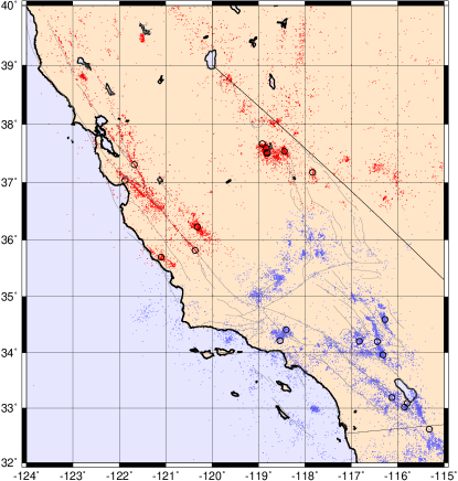
Figure 1: Map of earthquake ($m\geq 3$) epicenters in California from 1932 to the present. Circles are events with $m\geq 6$ since 1960. Red epicenters define the area used to analyze seismicity in northern California; blue epicenters define the area used for southern California.

The intensity change map builds upon the intensity map by computing the average squared change in intensity over a time interval $\Delta t=t_{2}-t_{1}$. Here we use $\Delta t=13$ years Rundle et al. (2002); Tiampo et al. (2002). We compute $n(\mathbf{x},t_{b},t_{1})$ and $n(\mathbf{x},t_{b},t_{2})$ for the two times $t_{1}$ and $t_{2}$, where $t_{2}>t_{1}$, beginning at a base time $t_{b}$, where $t_{1}>t_{b}>t_{0}$. Computing the change in numbers of events as $\Delta n(\mathbf{x},t_{b},t_{1},t_{2})=n(\mathbf{x},t_{b},t_{2})-n(\mathbf{x},t_{b},t_{1})$, we then define the intensity change $\Delta I(\mathbf{x},t_{1},t_{2})$ by normalizing $\Delta n(\mathbf{x},t_{b},t_{1},t_{2})$ to have spatial mean zero and unit variance, yielding $\Delta n^{\prime}(\mathbf{x},t_{b},t_{1},t_{2})$, and then averaging $\Delta n^{\prime}(\mathbf{x},t_{b},t_{1},t_{2})$ over all values for $t_{b}$ from $t_{0}$ to $t_{1}$: $\Delta I(\mathbf{x},t_{1},t_{2})=<\Delta n^{\prime}(\mathbf{x},t_{b},t_{1},t_{2})>_{t_{b}}$. The corresponding probability is $P_{\Delta}\equiv P_{\Delta}(\mathbf{x},t_{1},t_{2})=[\Delta I(\mathbf{x},t_{1},t_{2})]^{2}/\int[\Delta I(\mathbf{x},t_{1},t_{2})]^{2}\mathrm{d}\mathbf{x}$. Previous work Rundle et al. (2002); Tiampo et al. (2002); Holliday et al. (2005) has found that $P_{\Delta}$ is also a good predictor of locations for future large events having $m\geq 5$. $P_{\Delta}$ can be viewed as a probability based upon the squared change in intensity.

III Binary Forecasts

Binary forecasts are a well-known method for constructing forecasts of future event locations and have been widely used in tornado and severe storm forecasting Holliday et al. (2005); Jolliffe and Stephenson (2003). We construct binary forecasts for $m\geq m_{c}$ and for times $t>t_{2}$, where $m_{c}$ is a cutoff magnitude. In past work Rundle et al. (2002); Tiampo et al. (2002); Holliday et al. (2005) we have taken $m_{c}=5$, but we now remove this restriction. In our application, the probabilities $P_{\mu}\equiv P_{\mu}(\mathbf{x},t_{0},t_{2})$ and $P_{\Delta}\equiv P_{\Delta}(\mathbf{x},t_{1},t_{2})$ are converted to binary forecasts $B_{\mu}\equiv B_{\mu}(D,\mathbf{x},t_{0},t_{2})$ and $B_{\Delta}\equiv B_{\Delta}(D,\mathbf{x},t_{1},t_{2})$ by the use of a decision threshold $D$, where $D\in[0,\max\{P_{\mu}\}]$ or $D\in[0,\max\{P_{\Delta}\}]$ respectively Holliday et al. (2005); Jolliffe and Stephenson (2003).

For a given value of $D$, we set $B_{\mu}=1$ where $P_{\mu}>D$ and $B_{\mu}=0$ otherwise. Similarly, we set $B_{\Delta}=1$ where $P_{\Delta}>D$ and $B_{\Delta}=0$ otherwise. The set of pixels $\{\mathbf{x}_{\mu}(D)\}$ where $B_{\mu}=1$ and $\{\mathbf{x}_{\Delta}(D)\}$ where $B_{\Delta}=1$ then constitute locations where future events $m\geq m_{c}$ are considered to be likely to occur. We call these locations hotspots. The locations where $B_{\mu}=0$ and $B_{\Delta}=0$ are sites where future events $m\geq m_{c}$ are unlikely to occur. In previous work, intensity maps and intensity change maps at a particular value of $D$ were called Relative Intensity maps and Pattern Informatics maps. Examples of binary forecast maps are shown in Figure 2A.

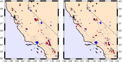
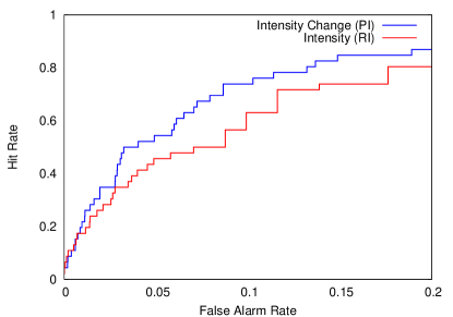
Figure 2: (A) $P_{\Delta}$ (intensity change) map (left) and $P_{\mu}$ (average intensity) map (right). A decision threshold $D$ was chosen leading to 75 hotspots in each map. Maps were computed for $t=$1 December 1994 with $t_{2}-t_{1}=13$ years. (B) ROC curves for $P_{\Delta}$ and $P_{\mu}$ corresponding to Figure 1. Here we have used $m_{c}=4$.

IV Receiver Operating Characteristic (ROC) Diagrams

A series of $D$-dependent contingency tables are constructed using the set of locations $\{\mathbf{x}_{q}(m_{c})\}$ where the $q=1,\ldots,Q$ large events $m\geq m_{c}$ are observed to actually occur during the forecast verification period $t>t_{2}$. The contingency table has 4 entries, $a\to d$, whose values are determined by some specified rule set Holliday et al. (2005); Jolliffe and Stephenson (2003). Here we use the following rules for given $D$ (same rules for both “$\mu$” and “$\Delta$” subscripts):

1. $a$ is the number of boxes in $\{\mathbf{x}(D)\}$ which are also in $\{\mathbf{x}_{q}(m_{c})\}$

2. $b$ is the number of boxes in $\{\mathbf{x}(D)\}$ whose location is not in $\{\mathbf{x}_{q}(m_{c})\}$, i.e., is in the complement to $\{\mathbf{x}_{q}(m_{c})\}$

3. $c$ is the number of boxes in the complement to $\{\mathbf{x}(D)\}$ whose location is in $\{\mathbf{x}_{q}(m_{c})\}$

4. $d$ is the number of boxes in the complement to $\{\mathbf{x}(D)\}$ whose locations are in the complement to $\{\mathbf{x}_{q}(m_{c})\}$

The hit rate is then defined as $H=a/(a+c)$, and the false alarm rate is defined as $F=b/(b+d)$. Note that with these definitions, $a+c=Q$, $a+b=$ number of hotspots, and $a+b+c+d=N$.

The ROC diagram Holliday et al. (2005); Jolliffe and Stephenson (2003) is a plot of the points $\{H,F\}$ as $D$ is varied. Examples of ROC curves corresponding to the intensity and intensity change maps in Figure 2A are shown in Figure 2B. A perfect forecast of occurrence (perfect order, no fluctuations) would consist of two line segments, the first connecting the points $(H,F)=(0,0)$ to $(H,F)=(1,0)$, and the second connecting $(H,F)=(1,0)$ to $(H,F)=(1,1)$. A curve of this type can be described as maximum possible hits ($H=1$) with minimum possible false alarms ($F=0$). Another type of perfect forecast (perfect order, no fluctuations) consists of two lines connecting the points $(0,0)$ to $(0,1)$ and $(0,1)$ to $(1,1)$, a perfect forecast of non-occurrence.

The line $H=F$ occupies a special status, and corresponds to a completely random forecast Holliday et al. (2005); Jolliffe and Stephenson (2003) (maximum disorder, maximum fluctuations) where the false alarm rate is the same as the hit rate and no information is produced by the forecast. Alternatively, we can say that the marginal utility Chung (1994) of an additional hotspot, $\mathrm{d}H/\mathrm{d}F$, equals unity for a random forecast.

For a given time-dependent forecast $H(F,t)$, we consider the time-dependent Pierce Skill Score $H(F,t)-F$ Jolliffe and Stephenson (2003), which measures the improvement in performance of $H(F,t)$ relative to the random forecast $H=F$. A Pierce function $\Psi(t)$ measures the area between $H(F,t)$ and the random forecast:

$$\Psi(t) = \int_{0}^{F_{\mathrm{max}}}(H(F,t)-F)\mathrm{d}F$$

$$= A(t)-F_{\mathrm{max}}^{2}/2,$$

where

$$A(t)=\int_{0}^{F_{\mathrm{max}}}H(F,t)\mathrm{d}F.$$ (2)

The upper limit $F_{\mathrm{max}}$ on the range if integration is a parameter whose value is set by the requirement that the marginal utility Chung (1994) of the forecast of occurrence $H(F,t)$ exceeds that of the random forecast $H=F$:

$$\frac{\mathrm{d}}{\mathrm{d}F}\{H(F,t)-F\}>0.$$ (3)

Since $H(F,t)$ curves are monotonically increasing, $F_{\mathrm{max}}$ is determined as the value of $F$ for which $\mathrm{d}H(F,t)/\mathrm{d}F=1$. For the forecasts we consider, we find that $F_{\mathrm{max}}\approx 0.2$, as can be seen from the examples in Figure 2B.

V Order Parameter and Generalized Ginzburg Criterion

We define an order parameter as the Pierce function $\Psi_{\tau}(t)$ obtained using as the probability $P_{\tau}\equiv P_{\tau}(\mathbf{x},t_{1},t_{2})=n(\mathbf{x},t_{1},t_{2})/\int n(\mathbf{x},t_{1},t_{2})\mathrm{d}\mathbf{x}$, where $P_{\tau}$ is the average normalized intensity of seismic activity during $t_{1}$ to $t_{2}$. Using $P_{\tau}$ and the decision threshold $D$, we construct a binary forecast $B_{\tau}\equiv B_{\tau}(D,\mathbf{x},t_{1},t_{2})$ . Evaluating the forecast $B_{\tau}$ during the time interval $t_{2}$ to $t$ produces the ROC diagram $H_{\tau}(F,t)$. For the case of forecasts having positive marginal utility relative to the random forecast, $\Psi_{\tau}(t)>0$. If past seismic activity is uncorrelated with future seismic activity, $P_{\tau}$ is equivalent to a random forecast, and $\Psi_{\tau}(t)=0$

Corresponding to the order parameter $\Psi_{\tau}(t)$, we define a function $\mathcal{G}(t)$ to indicate the relative importance of fluctuations with respect to forecasts of occurrence. We note that the probability $\Psi_{\Delta}$ is a measure of the mean squared change of intensity, a measure of fluctuations in seismic intensity, during $t_{1}$ to $t_{2}$, and that the probability $P_{\mu}$ is a measure of the average intensity over the entire time history ($t_{0}$ to $t_{2}$). We will refer to $P_{\Delta}$ as the “fluctuation map” or “change map”, and $P_{\mu}$ as the “average map”.

Using the corresponding ROC functions we define

$$\mathcal{G}(t)\equiv\frac{\Psi_{\Delta}(t)}{\Psi_{\mu}(t)},$$ (4)

where $\Psi_{\Delta}(t)$ is based upon the ROC curve computed using $P_{\Delta}$, $\{H_{\Delta}(F,t),F\}$ and $\Psi_{\mu}(t)$ is based upon the ROC curve computed using $P_{\mu}$, $\{H_{\mu}(F,t),F\}$. We can say that when $\mathcal{G}(t)<1$, “fluctuations are less significant relative to the mean” in the sense that the fluctuation map provides a poorer forecast than the mean map. This statement is equivalent to the Pierce difference function:

$$\Delta A(t)\equiv A_{\mu}(t)-A_{\Delta}(t)>0.$$ (5)

This difference function can be considered to be a generalized Ginzburg criterion Goldenfeld (1992).

To examine these ideas, we compare a plot of $\mathcal{G}(t)$ with activity of major earthquakes ($m\geq 6$) in California. We first consider the Gutenberg-Richter frequency-magnitude relation $f=10^{a}\cdot 10^{-bm}$, where $f$ is the number of events per unit time with magnitude larger than $m$ and $a$ and $b$ are constants. $a$ specifies the level of activity in the region, and $b\cong 1$.

To construct ROC curves, we consider $t$ to be the current time at each time step and test the average map and change map by forecasting locations of earthquakes during $t_{2}$ to $t$. We use events having $m\geq m_{T}$, where $m_{T}$ is some threshold magnitude. Note that $f^{-1}$ specifies a time scale for events larger than $m$: 1 event with $m\geq 6.0$ is associated on average with 10 $m\geq 5.0$ events, 100 $m\geq 4.0$ events, etc. Without prior knowledge of the optimal value for $m_{T}$, we average the results for a scale-invariant distribution of 1000 $m_{T}\geq 3.0$ events, 794 $m_{T}\geq 3.1$ events, 631 $m_{T}\geq 3.2$ events, $\ldots$, 10 $m_{T}\geq 5.0$ events. We terminate the sequence at $m_{T}\geq 5.0$ due to increasingly poor statistics. To control the number of earthquakes with $m\geq m_{T}$ in the snapshot window ($t_{2}$ to $t$), we determine the value of $t_{2}$ that most closely produces the desired number of events within the snapshot window. It is possible to have fluctuations in actual number of events if the snapshot window includes the occurrence time of a major earthquake, when there may be many events $m\geq m_{T}$ in the coarse-grained time intervals of length 1 day following the earthquake.

A central idea is that the length of the snapshot window is not fixed in time; it is instead fixed by earthquake number at each threshold magnitude $m_{T}=3.0,3.1,3.2$, and so forth. Nature appears to measure “earthquake time” in numbers of events, rather than in years. “Earthquake time” is evidently based on stress accumulation and release, that is, earthquake numbers, rather than in months or years Klein et al. (1997).

Results are shown in Figure 3 for the region of California shown in Figure 1. At top of either plot is the Pierce difference function $\Delta A(t)=A_{\mu}(t)-A_{\Delta}(t)$, and at bottom is earthquake magnitude plotted as a function of time from 1 January 1960 to 31 March 2006. The vertical lines in each top panel are the times of all events $m\geq 6$ in the region during that time interval. It can be seen from Figures 1 and 3 that there are 11 $m\geq 6$ events in northern California and 10 such events in southern California. For both areas, these major events are concentrated into 8 distinct “episodes” corresponding to 8 main shocks. In each plot, 7 of the 8 major episodes fall during (“black”) time intervals where $\Delta A(t)>0$, or they either begin or terminate such a time interval. If a binomial probability distribution is assumed, the chance that random clustering of these major earthquake episodes could produce this temporal concordance can be computed. For Figure 3A, where black time intervals constitute 36.8% of the total, we compute a 0.46% chance that the concordance is due to random clustering. For Figure 3B, the respective numbers are 19% of the total time interval, and 0.0058% chance due to random clustering. Our results support the prediction that major earthquake episodes preferentially occur during time intervals when fluctuations in seismic intensity, as measured by ROC curves, are less important than the average seismic intensity.

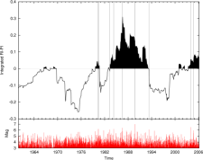
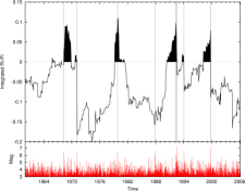
Figure 3: Value of the Pierce difference function $\Delta A(t)$ (top) and magnitude (bottom) as a function of time for events occurring on the map area of Figure 1. Vertical black lines represent times of major earthquakes having $m\geq 6$ in the respective regions. Differences are computed for a scale-invariant distribution of magnitude thresholds in the snapshot window from $m_{T}=3.0$ to $m_{T}=5.0$. Area integration is performed for $F\in[0.0,0.2]$. (A) Northern California (red epicenters in Figure 1). (B) Southern California (blue epicenters in Figure 1).