Stark effect of the cesium ground state:
electric tensor polarizability and shift of the clock transition frequency

Abstract

We present a theoretical analysis of the Stark effect in the hyperfine structure of the cesium ground-state. We have used third order perturbation theory, including diagonal and off-diagonal hyperfine interactions, and have identified terms which were not considered in earlier treatments. A numerical evaluation using perturbing levels up to $n=18$ yields new values for the tensor polarizability $\alpha_{2}(6S_{1/2})$ and for the Stark shift of the clock transition frequency in cesium. The polarizabilities are in good agreement with experimental values, thereby removing a 40-year-old discrepancy. The clock shift value is in excellent agreement with a recent measurement, but in contradiction with the commonly accepted value used to correct the black-body shift of primary frequency standards.

Since its discovery, the Stark effect has been an important spectroscopic tool for elucidating atomic structure. The Zeeman degeneracy of the $nS_{1/2}$ ground state of alkali atoms cannot be lifted by a static electric field because of time reversal invariance. However, the joint effect of the hyperfine interaction and the Stark interaction leads to both $F$ and $\left|M\right|$ dependent energy shifts which in cesium are 5 and 7 orders of magnitude smaller than the shift due to the second order scalar polarizability. While the scalar Stark shift is understood at a level of $\left(1\mbox{--}2\right)\cdot 10^{-3}$ Amini and Gould (2003); Derevianko and Porsev (2002); Zhou and Norcross (1989), there has so far been no satisfactory theoretical description of the $F$ and $\left|M\right|$ dependent alterations of the scalar effect at the levels of $10^{-5}$ and $10^{-7}$. In this Letter, we extend previous theoretical models which allows us to bridge a long standing gap between theory and experiment.

The effect of a static electric field on the hyperfine structure was treated in a comprehensive paper by Angel and Sandars Angel and H.Sandars (1968), who showed that the second order Stark effect of a state $\mathinner{|{\gamma}\rangle}=\mathinner{|{nL_{J},\,F,M}\rangle}$ can be parametrized in terms of a scalar polarizability, $\alpha_{0}^{(2)}(\gamma)$, and a tensor polarizability, $\alpha_{2}^{(2)}(\gamma)$, where the latter has non-zero values for states with $L~{}\geq~{}1$ only. As a consequence, the spherically symmetric $nS_{1/2}$ alkali-atom ground state has only a scalar polarizability, so that its magnetic sublevels $\mathinner{|{F,M}\rangle}$ all experience the same Stark shift, independent of $F$ and $M$. However, an experiment by Haun and Zacharias in 1957 Haun and Zacharias (1957) showed that a static electric field induces a quadratic (in field strength $\mathbb{E}$) shift of the $\mathinner{|{F=4,M=0}\rangle}\leftrightarrow\mathinner{|{F=3,M=0}\rangle}$ hyperfine (clock) transition frequency ($F$-dependent effect). In 1964, Lipworth and Sandars Lipworth and Sandars (1964) demonstrated that a static electric field also lifts the Zeeman degeneracy within the $F=4$ sublevel manifold of the cesium ground state ($M$-dependent effect). An improved measurement was performed later by Carrico et al. Carrico et al. (1968) and its extension to five stable alkali isotopes was done by Gould et al. Gould et al. (1969).

Sandars Sandars (1967) has shown that the $F$- and $M$-dependence of the Stark effect can be explained when the perturbation theory is extended to third order after including the hyperfine interaction. The theoretical expressions for the tensor polarizabilties $\alpha_{2}$ of Sandars (1967) were evaluated numerically in Lipworth and Sandars (1964) and Gould et al. (1969) under simplifying assumptions. Comparison with the experimental polarizabilities showed that the absolute theoretical values were systematically larger for all five alkalis studied in Gould et al. (1969). Our recent measurements Ospelkaus et al. (2003); Ulzega et al. ; Ulzega (2006) of $\alpha_{2}$ of ${}^{133}\text{Cs}$ confirmed the earlier experimental values Carrico et al. (1968); Gould et al. (1969). To help clarify this long-standing discrepancy we have reanalyzed the third-order calculation of the Stark effect in the alkali hyperfine structure. We have identified contributions which were not included in earlier calculations and as a result we obtain theoretical values which are in good agreement with experimental results Carrico et al. (1968); Gould et al. (1969); Ospelkaus et al. (2003); Ulzega et al. ; Ulzega (2006). When applied to the Stark shift of the clock transition frequency our calculations yield a value in good agreement with a recent measurement Godone et al. (2005).

The third order perturbation of the energy $E_{\alpha}$ of the sublevel $\mathinner{|{\alpha}\rangle}=\mathinner{|{6S_{1/2},F,M}\rangle}$ is given by

$$\Delta E^{(3)}(\alpha)=\sum_{\beta\neq\alpha,\gamma\neq\alpha}\frac{\left<\alpha\right|W\left|\beta\right>\left<\beta\right|W\left|\gamma\right>\left<\gamma\right|W\left|\alpha\right>}{(E_{\alpha}-E_{\beta})(E_{\alpha}-E_{\gamma})}\\ -\left<\alpha\right|W\left|\alpha\right>\sum_{\beta\neq\alpha}\frac{\left|\left<\beta\right|W\left|\alpha\right>\right|^{2}}{(E_{\alpha}-E_{\beta})^{2}}\>,$$ (1)

where $E_{\beta}$ and $E_{\gamma}$ are the energies of unperturbed states, and the perturbation $W=\mathrm{H}_{\mbox{\tiny hf}}+\mathrm{H}_{\mbox{\tiny St}}$ describes the hyperfine and Stark interactions. Of all the terms obtained by substituting W into Eq. (1) only those containing the product of two matrix elements of $\mathrm{H}_{\mbox{\tiny St}}$ and one matrix element of $\mathrm{H}_{\mbox{\tiny hf}}$ give nonzero contributions because of the selection rules $\Delta L=\pm 1$ for $\mathrm{H}_{\mbox{\tiny St}}$ and $\Delta L=0,\pm 2$ for $\mathrm{H}_{\mbox{\tiny hf}}$.

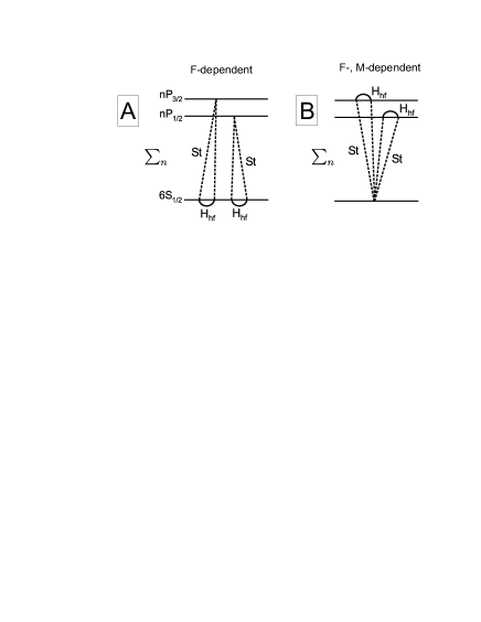
Figure 1: Contribution of diagonal hyperfine matrix elements to the third order Stark effect calculation. The dotted lines represent Stark interaction matrix elements while the solid lines represent hyperfine matrix elements.

We address first the second term of Eq. (1). The diagonal matrix element in front of the sum represents only the Fermi contact interaction in the ground state, while the sum is carried out over Stark interactions only. Diagram A of Fig. 1 represents this term in graphical form. The hyperfine matrix element $\mathinner{\langle{\alpha}|}\mathrm{H}_{\mbox{\tiny hf}}\mathinner{|{\alpha}\rangle}$ is scalar, but $F$ dependent, and the sum is similar to the expression for the second order polarizability, except for the squared energy denominator. As in the theory of the second order polarizability Angel and H.Sandars (1968) the sum can therefore be expressed as $\left<\alpha\right|\mathrm{H}_{\mbox{\tiny eff}}^{(k=0)}+\mathrm{H}_{\mbox{\tiny eff}}^{(k=2)}\left|\alpha\right>$. The scalar contribution, $\mathinner{\langle{\alpha}|}\mathrm{H}_{\mbox{\tiny eff}}^{(0)}\mathinner{|{\alpha}\rangle}$, depends only on the strength of the applied electric field, $\mathbb{E}^{2}$, while the second rank tensor contribution $\mathrm{H}_{\mbox{\tiny eff}}^{(2)}$ depends on its orientation as $3\mathbb{E}_{z}^{2}-\mathbb{E}^{2}$. The selection rules for tensor operators require that $\mathinner{\langle{S_{1/2}}\parallel}\mathrm{H}_{\mbox{\tiny eff}}^{(2)}\mathinner{\parallel{S_{1/2}}\rangle}=0$. As a consequence the second term of Eq. (1) gives a scalar contribution to the energy which depends on $F$, but not on $M$, and which can be parametrized by a third order scalar polarizability $\alpha_{0}^{(3)}(6S_{1/2},F)$ as

$$\Delta E^{(3)}_{0}(F)=-\frac{1}{2}\cdot\alpha_{0}^{(3)}(F)\cdot\mathbb{E}^{2}\,.$$ (2)

This term produces the major contribution to the Stark shift of the hyperfine transition frequency $\mathinner{\Delta}\nu_{00}\!=\!\nu(F\!=\!4,M\!=\!0)-\nu(F\!=\!3,M\!=\!0)$.

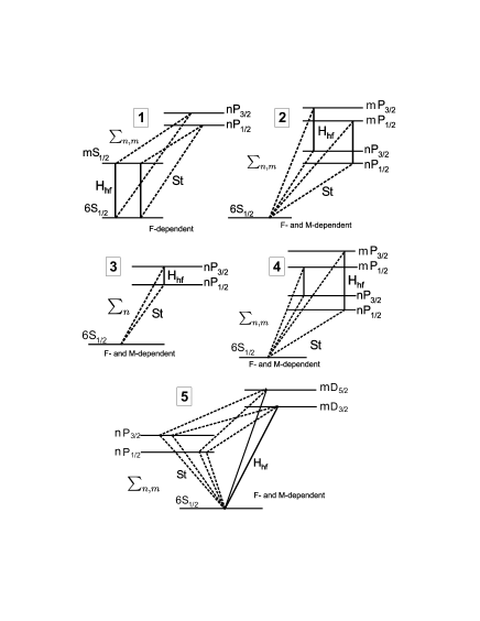
Figure 2: Contribution of off-diagonal hyperfine matrix elements to the third order calculation of the Stark effect.

We next address the first term of Eq. (1) and consider only diagonal matrix elements of $\mathrm{H}_{\mbox{\tiny hf}}$. As before, the Stark interaction part of the first term has only a rank $k=0$ (scalar) contribution. The dipole-dipole and electric quadrupole parts of the hyperfine interaction have the rotational symmetry of $k=0,2$ and $k=2$ tensors, respectively. Together with the scalar Stark interaction, the first term thus has scalar and tensor parts. The scalar part has the same $F$ dependence Ulzega (2006) as $\alpha_{0}^{(3)}(F)$, and corrects the latter by approximately 1%, while the second rank tensor parts have an $F$ and $M$ dependence, which can be parametrized in terms of a third order tensor polarizability $\alpha_{2}^{(3)}(6S_{1/2},F)$ via

$$\Delta E_{2}^{(3)}(\alpha)=-\frac{1}{2}\alpha_{2}^{(3)}(F)\frac{3M^{2}-F(F+1)}{2I(2I+1)}f(\theta)\mathbb{E}^{2}\,,$$ (3)

where the dependence on the angle $\theta$ between the electric field and the quantization axis is given by $f(\theta)=3\cos^{2}\theta-1$. The $M$-dependence in Eq. (3) is responsible for lifting the Zeeman degeneracy in the ground state hyperfine levels, but gives also a correction to the shift of the clock transition frequency which itself is dominated by Eq. (2). The third order Stark effect of the two hyperfine levels can then be parametrized in terms of the third order polarizabilities by

$$\alpha^{(3)}(F,M)=\alpha_{0}^{(3)}(F)+\alpha_{2}^{(3)}(F)\frac{3M^{2}\!-\!F(F\!+\!1)}{2I(2I+1)}f(\theta)\,.$$ (4)

In cesium the explicit $F$-dependence of Eq. (4) yields Ulzega et al. ; Ulzega (2006), for $\theta=0$,

$$\alpha^{(3)}(4,M)\! = \!a_{0}+\left(a_{1}+a_{2}\right)\frac{3M^{2}\!-\!20}{28}\>,$$ (5a)

$$\alpha^{(3)}(3,M)\! = \!-\frac{9}{7}a_{0}+\left(-a_{1}+\frac{5}{3}a_{2}\right)\frac{3M^{2}\!-\!12}{28}\>,$$ (5b)

where $a_{1}$ is the contribution of the tensor part of the dipole-dipole hyperfine interaction, and $a_{2}$ the contribution of the electric quadrupole interaction. The Fermi-contact interaction provides the dominant contribution to $a_{0}$ which also has a small contribution from the scalar part of the dipole-dipole interaction. Equations (5) bear a close resemblance to the expressions obtained by Sandars Sandars (1967), except for the negative sign of the $a_{1}$ term in Eq. (5b), which is positive in Sandars work. We have confirmed the sign of our expression in a recent experiment Ulzega et al. . That sign error, which seems to have remained unnoticed for almost 40 years, has no consequence for the tensor polarizability of the $F=4$ state, which is the only one measured to date. It affects the static Stark shift of the clock transition at a level slightly below today’s experimental sensitivity.

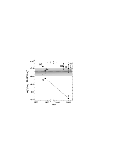
Figure 3: The third order tensor polarizability of the F=4 Cs ground state. The filled squares ($\blacksquare$) represent experimental values of Carrico et al. Carrico et al. (1968)(a), Gould et al. Gould et al. (1969)(b), Ospelkaus et al. Ospelkaus et al. (2003)(c) and Ulzega et al. Ulzega et al. (d). The empty square ($\square$) (e) represents a weighted average of (a), (b), (c) and (d). The dots (•) represent the theoretical value from Gould et al. (1969)(f), and our re-evaluation of the latter value after dropping simplifying assumptions (f’). The dotted horizontal line is the result of the present work with its uncertainty (shaded band).

Sandars’ equations were evaluated by Lipworth and Sandars (1964) and Gould et al. (1969) who considered only diagonal matrix elements of $\mathrm{H}_{\mbox{\tiny hf}}$ for the $6S_{1/2}$ and the $6P_{J}$ states (Fig. 1). They further neglected the fine structure energy splitting in the denominators of Eq. (1) and assumed the relation $A_{6P_{1/2}}=5A_{6P_{3/2}}$ for the hyperfine constants, valid for one-electron atoms, while for Cs the corresponding ratio of experimental values is 5.8. Those assumptions yielded the value (f) in Fig. 3, which is in disagreement with the experimental results. We have reevaluated Ulzega (2006) their result by dropping the simplifying assumptions and by using recent experimental values of the reduced matrix elements $\mathinner{\langle{6S_{1/2}}\parallel}d\mathinner{\parallel{6P_{j}}\rangle}$ from Rafac et al. (1994). As a result, the discrepancy becomes even larger [point (f’) in Fig. 3], and does not change significantly when the perturbation sum is extended to $nP_{J}$ states with $n>6$.

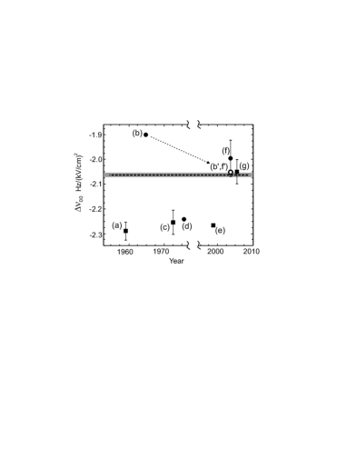
Figure 4: The static Stark shift of the clock transition frequency. The squares ($\blacksquare$) represent experimental values of Haun et al. Haun and Zacharias (1957)(a), Mowat Mowat (1972)(c), Simon et al. Simon et al. (1998)(e), and Godone et al. Godone et al. (2005)(g). The dots (•) represent theoretical values of Feichtner et al. Feichtner et al. (1965)(b), Lee et al. Lee et al. (1975)(d), and Micalizio et al. Micalizio et al. (2004)(f). The circle ($\circ$) (b’,f’) represents the rescaled values of (b,f) as explained in the text. The error bar of point (e) is smaller than the symbol size. The dotted horizontal line shows our result with its uncertainty (shaded band).

The first term in Eq. (1) is not restricted to diagonal matrix elements of the hyperfine interaction. We have therefore extended the numerical evaluation of Eq. (1) by including off-diagonal terms. Figure 2 gives a schematic overview of all possible configurations which include off-diagonal hyperfine matrix elements and which are compatible with the hyperfine and Stark operator selection rules. It is interesting to note that the diagrams 1 and 2 were already considered by Feichtner et al. Feichtner et al. (1965) in their calculation of the clock transition Stark shift. For unknown reasons, the off-diagonal terms were never included in the calculation of the tensor polarizability.

We have evaluated all the diagrams shown in Fig. 2, and in particular the diagrams 3, 4, and 5, which, to our knowledge, were never considered before. As noted in the figure, all diagrams lead to $F$ and $M$ dependent energy shifts, except for diagram 1, which gives an $M$ independent shift. Thus all diagrams contribute, together with the diagonal contributions A and B of Fig. 1, to the Stark shift of the clock transition, while only the diagrams B and 2–5 contribute to the tensor polarizability. Moreover, the relative importance of the diagrams for the two effects of interest is quite different. In the case of the clock shift, we find that 90% (95%) of the total contribution (n=$6\mbox{--}18$) comes from the diagrams A and 1 evaluated for $n=6,7$ ($n=6,7,8$). In this case the contributing (electric dipole and hyperfine) matrix elements are directly or indirectly given by experimentally measured quantities. The diagonal hyperfine matrix elements are proportional to the measured hyperfine splittings, while the off-diagonal hyperfine matrix elements between $S$ states of different principal quantum numbers $n$ can be expressed in terms of the geometrical averages of the hyperfine splittings of the coupled states, a relation which holds at a level of $10^{-3}$ Dzuba and Flambaum (2000). This gives us a high level of confidence in our value of the clock shift rate. The off-diagonal matrix elements of the diagrams 2–5 cannot be traced back to experimental quantities. We have calculated these matrix elements using wave functions obtained from the Schrödinger equation for a Thomas-Fermi potential, with corrections including dipolar and quadrupolar core polarization as well as spin-orbit interaction with a relativistic correction factor following Norcross (1973). We included $nS_{J}$, $nP_{J}$, and $nD_{J}$ states up to $n=18$ in the perturbation sum and obtained

$$\Delta\nu_{00}/\mathbb{E}^{2}=-2.06(1)\>\mbox{Hz}/(\mbox{kV}/\mbox{cm})^{2}\>,$$ (6)

for the shift of the clock transition frequency, and

$$\alpha_{2}^{(3)}(F=I\pm J)=\mp 3.72(25)\times 10^{-2}\>\mbox{Hz}/(\mbox{kV}/\mbox{cm})^{2}\>,$$ (7)

for the tensor polarizability. The results are shown as dotted lines in Figs. 3 and 4 together with previous theoretical and experimental results. The uncertainty of our calculated values is indicated by the shaded bands. The relative uncertainty of the clock shift is significantly smaller than that of the tensor polarizability due to the use of experimental values, with relatively small uncertainties. For the contributions which we calculated explicitly from the Schrödinger wave functions we use the accuracy (4%–8%) with which these wave functions reproduce experimental dipole matrix elements and hyperfine splittings to estimate the precision of our results. More details will be given in a forthcoming publication Ulzega et al. . We can claim that the present calculation of $\alpha_{2}^{(3)}$ yields a good agreement with all experimental data.

The situation with the Stark shift of the clock transition frequency is less clear as there are disagreeing experimental values. While the experimental results Haun and Zacharias (1957), Mowat (1972), and Simon et al. (1998) [(a), (c), and (e) in Fig. 4] are supported by the theoretical value of Lee et al. (1975)(d), our present result is in excellent agreement with the recent experimental value of Godone et al. Godone et al. (2005)(g) and with the calculation of Micalizio et al. Micalizio et al. (2004)(f). The shift was also calculated by Feichtner et al. Feichtner et al. (1965) in an approximation using hydrogenic wave functions, neglecting spin-orbit interactions, and considering only the diagrams A, B, 1, and 2 [point (b) in Fig. 4]. With these approximations the scalar polarizability $\alpha_{0}$ can be factored out of their final result. We have rescaled point (b) in Fig. 4 using more precise (consistent) values of $\alpha_{0}$ given in Amini and Gould (2003); Derevianko and Porsev (2002); Zhou and Norcross (1989), yielding point (b’) which is then consistent with the present result. We also rescaled point (f) in the same manner, yielding (f’) which cannot be distinguished from (b’).

We conclude by recalling the relevance of the latter result for primary frequency standards. One of the leading systematic shifts of the cesium clock frequency is due to the interaction of the atoms with the blackbody radiation (BBR) field. It was shown Itano et al. (1982) that the dynamic BBR shift can be parametrized in terms of the static Stark shift investigated here. The correction factor for the BBR shift commonly used is based on the precise experimental value of Simon et al. Simon et al. (1998) [point (e) in Fig. 4], whose difference with the present result is 21 (53) times the corresponding theoretical (experimental) uncertainty. In order to shine more light on this important issue we are preparing an alternative new experiment for measuring the static Stark shift of the clock transition frequency.

The authors acknowledge a partial funding of the present work by Swiss National Science Foundation (grant 200020–103864). One of us (A.W.) thanks M.-A. Bouchiat for useful discussions.

References

- Amini and Gould (2003) J. M. Amini and H. Gould, Phys. Rev. Lett. 91, 153001 (2003).
- Derevianko and Porsev (2002) A. Derevianko and S. G. Porsev, Phys. Rev. A 65, 053403 (2002).
- Zhou and Norcross (1989) H. L. Zhou and D. W. Norcross, Phys. Rev. A 40, 5048 (1989).
- Angel and H.Sandars (1968) J. R. P. Angel and P. G. H.Sandars, Proc. R. Soc. London, A 305, 125 (1968).
- Haun and Zacharias (1957) R. D. Haun and J. R. Zacharias, Phys. Rev. 107, 107 (1957).
- Lipworth and Sandars (1964) E. Lipworth and P. G. H. Sandars, Phys. Rev. Lett. 13, 716 (1964).
- Carrico et al. (1968) J. P. Carrico, A. Adler, M. R. Baker, S. Legowski, E. Lipworth, P. G. H. Sandars, T. S. Stein, and C. Weisskopf, Phys. Rev. 170, 64 (1968).
- Gould et al. (1969) H. Gould, E. Lipworth, and M. C. Weisskopf, Phys. Rev. 188, 24 (1969).
- Sandars (1967) P. G. H. Sandars, Proc. Phys. Soc. 92, 857 (1967).
- Ospelkaus et al. (2003) C. Ospelkaus, U. Rasbach, and A. Weis, Phys. Rev. A 67, 011402 (2003).
- (11) S. Ulzega, A. Hofer, P. Moroshkin, and A. Weis, to be published.
- Ulzega (2006) S. Ulzega, Ph.D. thesis, University of Fribourg, Switzerland (2006).
- Godone et al. (2005) A. Godone, D. Calonico, F. Levi, S. Micalizio, and C. Calosso, Phys. Rev. A 71, 063401 (2005).
- Rafac et al. (1994) R. J. Rafac, C. E. Tanner, A. E. Livingston, K. W. Kukla, H. G. Berry, and C. A. Kurtz, Phys. Rev. A 50, 1976 (1994).
- Mowat (1972) J. R. Mowat, Phys. Rev. A 5, 1059 (1972).
- Simon et al. (1998) E. Simon, P. Laurent, and A. Clairon, Phys. Rev. A 57, 436 (1998).
- Feichtner et al. (1965) J. D. Feichtner, M. E. Hoover, and M. Mizushima, Phys. Rev. 137, A702 (1965).
- Lee et al. (1975) T. Lee, T. P. Das, and R. M. Sternheimer, Phys. Rev. A 11, 1784 (1975).
- Micalizio et al. (2004) S. Micalizio, A. Godone, D. Calonico, F. Levi, and L. Lorini, Phys. Rev. A 69, 053401 (2004).
- Dzuba and Flambaum (2000) V. A. Dzuba and V. V. Flambaum, Phys. Rev. A 62, 052101 (2000).
- Norcross (1973) D. W. Norcross, Phys. Rev. A 7, 606 (1973).
- Itano et al. (1982) W. M. Itano, L. L. Lewis, and D. J. Wineland, Phys. Rev. A 25 (1982).