Dynamics of Multi-Player Games

Abstract

We analyze the dynamics of competitions with a large number of players. In our model, $n$ players compete against each other and the winner is decided based on the standings: in each competition, the $m$th ranked player wins. We solve for the long time limit of the distribution of the number of wins for all $n$ and $m$ and find three different scenarios. When the best player wins, the standings are most competitive as there is one-tier with a clear differentiation between strong and weak players. When an intermediate player wins, the standings are two-tier with equally-strong players in the top tier and clearly-separated players in the lower tier. When the worst player wins, the standings are least competitive as there is one tier in which all of the players are equal. This behavior is understood via scaling analysis of the nonlinear evolution equations.

I Introduction

Interacting particle or agent-based techniques are a central method in the physics of complex systems. This methodology heavily relies on the dynamics of the agents or the interactions between the agents, as defined on a microscopic level ww . In this respect, this approach is orthogonal to the traditional game theoretic framework that is based on the global utility or function of the system, as defined on a macroscopic level ft .

Such physics-inspired approaches, where agents are treated as particles in a physical system, have recently led to quantitative predictions in a wide variety of social and economic systems hfv ; ckfl ; bvr . Current areas of interest include the distribution of income and wealth ikr ; dy ; fs ; sr , opinion dynamics wdan ; smo ; bkr , the propagation of innovation and ideas dz , and the emergence of social hierarchies btd ; ss ; msk ; br .

In the latter example, most relevant to this study, competition is the mechanism responsible for the emergence of disparate social classes in human and animal communities. A recently introduced competition process btd ; br is based on two-player competitions where the stronger player wins with a fixed probability and the weaker player wins with a smaller probability bvr1 . This theory has proved to be useful for understanding major team sports and for analysis of game results data bvr .

In this study, we consider multi-player games and address the situation where the outcome of a game is completely deterministic. In our model, a large number of players $n$ participate in the game, and in each competition, the $m$th ranked player always wins. The number of wins measures the strength of a player. Furthermore, the distribution of the number of wins characterizes the nature of the standings. We address the time-evolution of this distribution using the rate equation approach, and then, solve for the long-time asymptotic behavior using scaling techniques.

Our main result is that there are three types of standings. When the best player wins, $m=1$, there is a clear notion of player strength; the higher the ranking the larger the winning rate. When an intermediate player wins, $1<m<n$, the standings have two tiers. Players in the lower tier are well separated, but players in the upper-tier are all equally strong. When the weakest player wins, $m=n$, the lower tier disappears and all of the players are equal in strength. In this sense, when the best player wins, the environment is most competitive, and when the worst player wins it is the least competitive.

The rest of this paper is organized as follows. We introduce the model in section II. In Section III, we analyze in detail three-player competitions, addressing situations where the best, intermediate, and worst player wins, in order. We then consider games with an arbitrary number of players and pay special attention to the large-$n$ limit in Section IV. We conclude in section V.

II The multi-player model

Our system consists of $N$ players that compete against each other. In each competition $n$ players are randomly chosen from the total pool of players. The winner is decided based upon the ranking: the $m$th ranked player always wins the game [Fig. 1]. Let $k_{i}$ be the number of wins of the $i$th ranked player in the competition, i.e., $k_{1}\geq\cdots\geq k_{m}\geq\cdots\geq k_{n}$, then

$$(k_{1},\ldots,k_{m},\ldots k_{n})\to(k_{1},\ldots,k_{m}+1,\ldots,k_{n}).$$ (1)

Tie-breakers are decided by a coin-toss, i.e., when two or more players are tied, their relative ranking is determined in a completely random fashion. Initially, players start with no wins, $k=0$.

Figure 1: Illustration of the multiplayer game with $n=5$ and $m=3$.

These competition rules are relevant in a wide variety of contexts. In sports competitions, the strongest player often emerges as the winner. In social contexts and especially in politics, being a centrist often pays off, and furthermore, there are auctions where the second highest bidder wins. Finally, identifying wins with financial assets, the situation where the weakest player wins mimics a strong welfare system where the rich support the poor.

We set the competition rate such that the number of competitions in a unit time equals the total number of players. Thence, each player participates in $n$ games per unit time, and furthermore, the average number of wins $\langle k\rangle$ simply equals time

$$\langle k\rangle=t.$$ (2)

At large times, it is natural to analyze the winning rate, that is, the number of wins normalized by time, $x=k/t$. Similarly, from our definition of the competition rate, the average winning rate equals one

$$\langle x\rangle=1.$$ (3)

Our goal is to characterize how the number of wins, or alternatively, the winning rate are distributed in the long time limit. We note that since the players are randomly chosen in each competition, the number of games played by a given player is a fluctuating quantity. Nevertheless, since this process is completely random, fluctuations in the number of games played by a given player scale as the square-root of time, and thus, these fluctuations become irrelevant in the long time limit. Also, we consider the thermodynamic limit, $N\to\infty$.

III Three player games

We first analyze the three player case, $n=3$, because it nicely demonstrates the full spectrum of possibilities. We detail the three scenarios where the best, intermediate, and worst, players win in order.

III.1 Best player wins

Let us first analyze the case where the best player wins. That is, if the number of wins of the three players are $k_{1}\geq k_{2}\geq k_{3}$, then the game outcome is as follows

$$(k_{1},k_{2},k_{3})\to(k_{1}+1,k_{2},k_{3}).$$ (4)

Let $f_{k}(t)$ be the probability distribution of players with $k\geq 0$ wins at time $t$. This distribution is properly normalized, $\sum_{k}f_{k}=1$, and it evolves according to the nonlinear difference-differential equation

$$\frac{df_{k}}{dt} = {3\choose 1}(f_{k-1}F^{2}_{k-1}-f_{k}\,F^{2}_{k})$$

$$+ {3\choose 2}\left(f^{2}_{k-1}F_{k-1}-f^{2}_{k}\,F_{k}\right)$$

$$+ {3\choose 3}\left(f^{3}_{k-1}-f^{3}_{k}\right).$$

Here, we used the cumulative distributions $F_{k}=\sum_{j=0}^{k-1}f_{j}$ and $G_{k}=\sum_{j=k+1}^{\infty}f_{j}$ of players with fitness smaller than and larger than $k$, respectively. The two cumulative distributions are of course related, $F_{k}+G_{k-1}=1$. The first pair of terms accounts for games where it is unambiguous who the top player is. The next pair accounts for two-way ties for first, and the last pair for three way ties. Each pair of terms contains a gain term and a loss term that differ by a simple index shift. The binomial coefficients account for the number of distinct ways there are to choose the players. For example, there are ${3\choose 1}=3$ ways to choose the top player in the first case. This master equation should be solved subject to the initial condition $f_{k}(0)=\delta_{k,0}$ and the boundary condition $f_{-1}(t)=0$. One can verify by summing the equations that the total probability is conserved $\frac{d}{dt}\sum_{k}f_{k}=0$, and that the average fitness $\langle k\rangle=\sum_{k}kf_{k}$ evolves as in (2), $d\langle k\rangle/dt=1$.

For theoretical analysis, it is convenient to study the cumulative distribution $F_{k}$. Summing the rate equations (III.1), we obtain closed equations for the cumulative distribution

$$\frac{dF_{k}}{dt} = -3(F_{k}-F_{k-1})F^{2}_{k-1}$$

$$-3(F_{k}-F_{k-1})^{2}F_{k-1}$$

$$-(F_{k}-F_{k-1})^{3}.$$

Here, we used $f_{k}=F_{k+1}-F_{k}$. This master equation is subject to the initial condition $F_{k}(0)=1$ and the boundary condition $F_{-1}(t)=0$.

We are interested in the long time limit. Since the number of wins is expected to grow linearly with time, $k\sim t$, we may treat the number of wins as a continuous variable, $F_{k-1}=F_{k}-\frac{\partial F}{\partial k}+\frac{1}{2}\frac{\partial^{2}F}{\partial k^{2}}+\cdots$. Asymptotically, since $\frac{\partial F}{\partial k}\propto t^{-1}$ and $\frac{\partial^{2}F}{\partial k^{2}}\propto t^{-2}$, etc., second- and higher-order terms become negligible compared with the first order terms. To leading order, the cumulative distribution obeys the following partial differential equation

$$\frac{\partial F}{\partial t}+3F^{2}\frac{\partial F}{\partial k}=0.$$ (7)

From dimensional analysis of this equation, we anticipate that the cumulative distribution obeys the scaling form

$$F_{k}(t)\simeq\Phi(k/t)$$ (8)

with the boundary conditions $\Phi(0)=0$ and $\Phi(\infty)=1$. In other words, instead of concentrating on the number of wins $k$, we focus on the winning rate $x=k/t$. In the long time limit, the cumulative distribution of winning rates $\Phi(x)$ becomes stationary. Of course, the actual distribution of winning rates $\phi(x)$ also becomes stationary, and it is related to the distribution of the number of wins by the scaling transformation

$$f_{k}(t)\simeq t^{-1}\phi(k/t)$$ (9)

with $\phi(x)=\Phi^{\prime}(x)$. Since the average winning rate equals one (3), the distribution of winning rates must satisfy

$$1=\int_{0}^{\infty}dx\,x\,\Phi^{\prime}(x).$$ (10)

Substituting the definition (8) into the master equation (7), the stationary distribution satisfies

$$\Phi^{\prime}(x)[3\Phi^{2}-x]=0.$$ (11)

There are two solutions: (i) The constant solution, $\Phi(x)={\rm const}$, and (ii) The algebraic solution $\Phi_{s}(x)=(x/3)^{1/3}$. Invoking the boundary condition $\lim_{x\to\infty}\Phi(x)=1$ we find [Fig. 2]

$$\Phi(x)=\begin{cases}(x/3)^{1/2}&x\leq 3\\ 1&x\geq 3.\\ \end{cases}$$ (12)

One can verify that this stationary distribution satisfies the constraint (10) so that the average winning rate equals one. This result generalizes the linear stationary distribution found for two player games br .

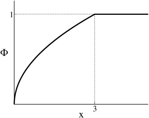
Figure 2: The stationary distribution of winning rates (12) for the case $n=3$, $m=1$.

Initially, all the players are identical, but by the random competition process, some players end up at the top of the standings and some at the bottom. This directly follows from the fact that the distribution of winning rates is nontrivial. Also, since $\phi(x)\sim x^{-1/2}$ as $x\to 0$, the distribution of winning-rate is nonuniform and there are many more players with very low winning rates. When the number of players is finite, a clear ranking emerges, and every player wins at a different rate. Moreover, after a transient regime, the rankings do not change with time [Fig. 3].

Figure 3: Schematic illustration of the number of wins $k$ versus time $t$ when the best player wins. Shown are results of simulations with 20 players.

We note that in our scaling analysis, situations where there is a two- or three-way tie for first do not contribute. This is the case because the number of wins grows linearly with time and therefore, the probability of finding two players with the same number of wins can be neglected. Such terms do affect how the distribution of the number of wins approaches a stationary form, but they do not affect the final form of the stationary distribution.

III.2 Intermediate player wins

Next, we address the case where the intermediate player wins,

$$(k_{1},k_{2},k_{3})\to(k_{1},k_{2}+1,k_{3}).$$ (13)

Now, there are four terms in the master equation

$$\frac{df_{k}}{dt} = {3\choose 1}{2\choose 1}(f_{k-1}F_{k-1}G_{k-1}-f_{k}F_{k}G_{k})$$

$$+ {3\choose 1}\left(f^{2}_{k-1}G_{k-1}-f^{2}_{k}\,G_{k}\right)$$

$$+ {3\choose 2}\left(f^{2}_{k-1}F_{k-1}-f^{2}_{k}\,F_{k}\right)$$

$$+ {3\choose 3}\left(f^{3}_{k-1}-f^{3}_{k}\right).$$

The first pair of terms accounts for situations where there are no ties and then the combinatorial prefactor is a product of the number of ways to choose the intermediate player times the number of ways to choose the best player. The next two pairs of terms account for situations where there is a two-way tie for best and worst, respectively. Again, the last pair of terms accounts for three-way ties. These equations conserve the total probability, $\sum_{k}f_{k}=1$, and they are also consistent with (2).

Summing the rate equations (III.2), we obtain closed equations for the cumulative distribution

$$\frac{dF_{k}}{dt} = -6(F_{k}-F_{k-1})F_{k-1}G_{k-1}$$

$$-3(F_{k}-F_{k-1})^{2}(F_{k-1}+G_{k-1})$$

$$-(F_{k}-F_{k-1})^{3}.$$

For clarity, we use both of the cumulative distributions, but note that this equation is definitely closed in $F_{k}$ because of the relation $G_{k}=1-F_{k+1}$. Taking the continuum limit and keeping only first-order derivatives, the cumulative distribution obeys the following partial differential equation $\frac{\partial F}{\partial t}+6F(1-F)\frac{\partial F}{\partial k}=0$ with the boundary conditions $F_{0}=0$ and $\lim_{k\to\infty}F_{k}=1$. Substituting the definition of the stationary distribution of winning rates (8) into this partial differential equation, we arrive at

$$\Phi^{\prime}(x)[6\Phi(1-\Phi)-x]=0,$$ (16)

an equation that is subject to the boundary conditions $\Phi(0)=0$ and $\lim_{x\to\infty}\Phi(x)=1$. There are two solutions: (i) The constant solution, $\Phi(x)={\rm const}$, and (ii) The root of the second-order polynomial $\Phi_{s}(x)=\frac{1}{2}\big{(}1-\sqrt{1-2x/3}\big{)}$. Invoking the boundary conditions, we conclude [Fig. 4]

$$\Phi(x)=\begin{cases}\frac{1}{2}\left(1-\sqrt{1-\frac{2}{3}x}\right)&x<x_{0}\\ 1&x>x_{0}.\\ \end{cases}$$ (17)

As the nontrivial solution is bounded $\Phi_{s}(x)\leq 1/2$, the cumulative distribution must have a discontinuity. We have implicitly assumed that this discontinuity is located at $x_{0}<3/2$.

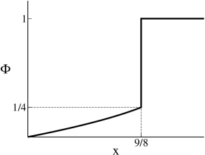
Figure 4: The stationary distribution of winning rates (17) for $n=3$, $m=2$.

The location of this discontinuity is dictated by the average number of wins constraint. Substituting the stationary distribution (17) into (10) then

$$1=\int_{0}^{x_{0}}dx\,x\,\Phi^{\prime}(x)+x_{0}[1-\Phi(x_{0})].$$

In writing this equality, we utilized the fact that the stationary distribution has a discontinuity at $x_{0}$ and that the size of this discontinuity is $1-\Phi_{0}$. Integrating by parts, we obtain an implicit equation for the location of the discontinuity

$$1=x_{0}-\int_{0}^{x_{0}}\,dx\,\Phi(x).$$ (18)

Substituting the stationary solution (17) into this equation and performing the integration, we find after several manipulations that the location of the singularity satisfies the cubic equation $x_{0}^{2}\big{(}x_{0}-\frac{9}{8}\big{)}=0$. The location of the discontinuity is therefore

$$x_{0}=\frac{9}{8}.$$ (19)

This completes the solution (17) for the scaling function. The size of the discontinuity follows from $\Phi_{0}\equiv\Phi(x_{0})=1/4$.

Figure 5: Schematic illustration of the number of wins $k$ versus time $t$ when the intermediate player wins. Shown are results of simulations with 20 players.

There is an alternative way to find the location of the discontinuity. Let us transform the integration over $x$ into an integration over $\Phi$ using the equality

$$x_{0}\Phi_{0} = \int_{0}^{x_{0}}\,dx\,\Phi(x)+\int_{0}^{\Phi_{0}}d\Phi\,x(\Phi).$$ (20)

This transforms the equation for the location of the discontinuity (18) into an equation for the size of the jump

$$1=x_{0}(1-\Phi_{0})+\int_{0}^{\Phi_{0}}\,d\Phi\,x(\Phi).$$ (21)

Substituting $x(\Phi)=6\Phi(1-\Phi)$ we arrive at the cubic equation for the variable $\Phi_{0}$, $1=6\Phi_{0}-9\Phi_{0}^{2}+4\Phi_{0}^{3}$. The relevant solution is $\Phi_{0}=\frac{1}{4}$, from which we conclude $x_{0}=9/8$. For three-player games, there is no particular advantage for either of the two approaches: both (18) and (21) involve cubic polynomials. However, in general, the latter approach is superior because it does not require an explicit solution for $\Phi(x)$.

The scaling function corresponding to the win-number distribution is therefore

$$\phi(x)=\frac{1}{6}\,\left({1-\frac{2}{3}\,x\,}\right)^{-1/2}\,+\,\frac{3}{4}\,\delta\left(x-\frac{9}{8}\right),$$

where $\delta(x)$ denotes the Kronecker delta function. The win-number distribution contains two components. The first is a nontrivial distribution of players with winning rate $x<x_{0}$ and the second reflects that a finite fraction of the players have the maximal winning rate $x=x_{0}$. Thus, the standings have a two-tier structure. Players in the lower tier have different strengths and there is a clear differentiation among them [Fig. 5]. Players in the upper-tier are essentially equal in strength as they all win with the same rate. A fraction $\Phi_{0}=\frac{1}{4}$ belongs to the lower tier and a complementary fraction $1-\Phi_{0}=\frac{3}{4}$ belongs to the upper tier. Interestingly, the upper-tier has the form of a condensate. We note that a condensate, located at the bottom, rather than at the top as is the case here, was found in the diversity model in Ref. br .

III.3 Worst player wins

Last, we address the case where the worst player wins bvr1 ; ktnr

$$(k_{1},k_{2},k_{3})\to(k_{1},k_{2},k_{3}+1).$$ (22)

Here, the distribution of the number of wins evolves according to

$$\frac{df_{k}}{dt} = {3\choose 1}(f_{k-1}G^{2}_{k-1}-f_{k}\,G^{2}_{k})$$

$$+ {3\choose 2}\left(f^{2}_{k-1}G_{k-1}-f^{2}_{k}\,G_{k}\right)$$

$$+ {3\choose 3}\left(f^{3}_{k-1}-f^{3}_{k}\right).$$

This equation is obtained from (III.1) simply by replacing the cumulative distribution $F_{k}$ with $G_{k}$. The closed equation for the cumulative distribution is now

$$\frac{dF_{k}}{dt} = -3(F_{k}-F_{k-1})G^{2}_{k-1}$$

$$-3(F_{k}-F_{k-1})^{2}G_{k-1}$$

$$-(F_{k}-F_{k-1})^{3}.$$

In the continuum limit, this equation becomes $\frac{\partial F}{\partial t}+3(1-F)^{2}\frac{\partial F}{\partial k}=0$, and consequently, the stationary distribution satisfies

$$\Phi^{\prime}(x)[3(1-\Phi)^{2}-x]=0.$$ (25)

Now, there is only one solution, the constant $\Phi(x)={\rm const}$, and because of the boundary conditions $\Phi(0)=0$ and $\lim_{x\to\infty}\Phi(x)=1$, the stationary distribution is a step function: $\Phi(x)=1$ for $x>x_{0}$ and $\Phi(x)=0$ for $x<x_{0}$. In other words, $\Phi(x)=\Theta(x-x_{0})$. Substituting this form into the condition (10), the location of the discontinuity is simply $x_{0}=1$, and therefore [Fig. 6]

$$\Phi(x)=\Theta(x-1)$$ (26)

where $\Theta(x)$ is the Heaviside step function. When the worst player wins, the standings no longer contain a lower-tier: they consist only of an upper-tier where all players have the same winning rate, $\phi(x)=\delta(x-1)$.

Figure 6: The stationary distribution of winning rates (26) for the case $n=m=3$.

IV Arbitrary number of players

Let us now consider the most general case where there are $n$ players and the $m$th ranked player wins as in (1). It is straightforward to generalize the rate equations for the cumulative distribution. Repeating the scaling analysis above, Eqs. (11) and (16) for the stationary distribution (8) generalize as follows:

$$\Phi^{\prime}(x)[C\Phi^{n-m}(1-\Phi)^{m-1}-x]=0.$$ (27)

The constant $C$ equals the number of ways to choose the $m$th ranked player times the number of ways to choose the $m-1$ higher ranked players

$$C={n\choose 1}{n-1\choose m-1}=\frac{n!}{(n-m)!(m-1)!}.$$ (28)

Again, there are two solutions: (i) The constant solution, $\Phi^{\prime}(x)=0$, and (ii) The root of the $(n-1)$th-order polynomial

$$C\Phi^{n-m}(1-\Phi)^{m-1}=x.$$ (29)

We now analyze the three cases where the best, an intermediate, and the worst player win, in order.

Best player wins ($m=1$): In this case, the stationary distribution can be calculated analytically,

$$\Phi(x)=\begin{cases}(x/n)^{1/(n-1)}&x\leq n;\\ 1&x\geq n.\end{cases}$$ (30)

One can verify that this solution is consistent with (3). We see that in general, when the best player wins there is no discontinuity and $\Phi_{0}=1$. As for three-player games, the standings consist of a single tier where some players rank high and some rank low. Also, the winning rate of the top players equals the number of players, $x_{0}=n$. In general, the distribution of the number of wins is algebraic.

Intermediate player wins ($1<m<n$): Based on the behavior for three player games, we expect

$$\Phi(x)=\begin{cases}\Phi_{s}(x)&x<x_{0};\\ 1&x\geq x_{0}.\end{cases}$$ (31)

Here, $\Phi_{s}(x)$ is the solution of (29). Numerical simulations confirm this behavior [Fig. 7]. Thus, we conclude that in general, there are two tiers. In the upper tier, all players have the same winning rate, while in the lower tier different players win at different rates. Generally, a finite fraction $\Phi_{0}$ belongs to the lower tier and the complementary fraction $1-\Phi_{0}$ belongs to the upper tier.

Our Monte Carlo simulations are performed by simply mimicking the competition process. The system consists of a large number of players $N$, all starting with no wins. In each elemental step, $n$ players are chosen and ranked and the $m$th ranked player is awarded a win (tied players are ranked in a random fashion). Time is augmented by $1/N$ after each such step. This elemental step is then repeated.

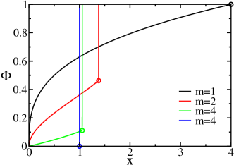
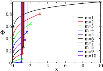
Figure 7: The stationary distribution of winning rates $\Phi(x)$ for $n=4$ (top) and $n=10$ (bottom). Shown are Monte Carlo simulation results with $N=10^{6}$ particles at time $t=10^{5}$. The circles are the theoretical predictions for the maximal winning rate $x_{0}$ and the size of the lower tier $\Phi_{0}$.

The parameters $x_{0}$ and $\Phi_{0}$ characterize two important properties: the maximal winning rate and the size of each tier. Thus, we focus on the behavior of these two parameters and pay special attention to the large-$n$ limit. Substituting the stationary distribution (31) into the constraint (10), the maximal winning rate $x_{0}$ follows from the very same Eq. (18). Similarly, the size of the lower tier follows from Eq. (21). In this case, the latter is a polynomial of degree $n+1$, so numerically, one solves first for $\Phi_{0}$ and then uses (29) to obtain $x_{0}$. We verified these theoretical predictions for the cases $n=4$ and $n=10$ using Monte Carlo simulations [Fig. 7].

For completeness, we mention that it is possible to rewrite Eq. (21) in a compact form. Using the definition of the Beta function

$$\int_{0}^{1}d\Phi\,\Phi^{n-m}(1-\Phi)^{m-1} = B(n-m+1,m)$$

$$= \frac{(n-m)!(m-1)!}{n!}$$

$$= C^{-1}$$

we relate the definite integral above with the combinatorial constant in (28). Substituting the governing equation for the stationary distribution (29) into the equation for the size of the lower-tier (21) gives

$$C^{-1}=\Phi_{0}^{n-m}(1-\Phi_{0})^{m}+\int_{0}^{\Phi_{0}}d\Phi\,\Phi^{n-m}(1-\Phi)^{m-1}.$$ (33)

Using the relation (IV), we arrive at a convenient equation for the size of the lower tier $\Phi_{0}$

$$\int_{\Phi_{0}}^{1}d\Phi\,\Phi^{n-m}(1-\Phi)^{m-1}=\Phi_{0}^{n-m}(1-\Phi_{0})^{m}.$$ (34)

This is a polynomial of degree $n+1$.

Let us consider the limit $n\to\infty$ and $m\to\infty$ with the ratio $\alpha=m/n$ kept constant. For example, the case $\alpha=1/2$ corresponds to the situation where the median player is the winner. To solve the governing equation for the stationary distribution in the large-$n$ limit, we estimate the combinatorial constant $C$ using Eq. (28) and the Stirling formula $n!\sim(2\pi n)^{1/2}(n/e)^{n}$. Eq. (29) becomes

$$\sqrt{\frac{n\alpha}{2\pi(1-\alpha)}}\left(\frac{\Phi}{1-\alpha}\right)^{n-m}\left(\frac{1-\Phi}{\alpha}\right)^{m-1}\sim x.$$ (35)

Taking the power $1/n$ on both sides of this equation, and then the limit $n\to\infty$, we arrive at the very simple equation,

$$\Big{(}\frac{\Phi}{1-\alpha}\Big{)}^{1-\alpha}\Big{(}\frac{1-\Phi}{\alpha}\Big{)}^{\alpha}=1.$$ (36)

By inspection, the solution is constant, $\Phi=1-\alpha$. Using $\Phi_{0}=1-\alpha$ and employing the condition $\langle x\rangle=1$ yields the location of the condensate

$$x_{0}=1/\alpha,\qquad\Phi_{0}=1-\alpha.$$ (37)

This result is consistent with the expected behaviors $x_{0}\to\infty$ as $\alpha\to 0$ and $x_{0}(\alpha=1)=1$ (see the worst player wins discussion below). Therefore, the stationary distribution contains two steps when the number of players participating in each game diverges [Fig. 8]

$$\Phi(x)=\begin{cases}0&x<0\\ 1-\alpha&0<x<\alpha^{-1}\\ 1&\alpha^{-1}<x.\end{cases}$$ (38)

The stationary distribution corresponding to the number of wins therefore consists of two delta-functions: $\phi(x)=(1-\alpha)\delta(x)+\alpha\delta(x-1/\alpha)$. Thus, as the number of players participating in a game grows, the winning rate of players in the lower tier diminishes, and eventually, they become indistinguishable.

For example, for $n=10$, the quantity $\Phi_{0}$ is roughly linear in $\alpha$ and the maximal winning rate $x_{0}$ is roughly proportional to $\alpha^{-1}$ [Fig. 7]. Nevertheless, for moderate $n$ there are still significant deviations from the limiting asymptotic behavior. A refined asymptotic analysis shows that $\Phi_{0}-(1-\alpha)\sim\sqrt{\alpha(1-\alpha)\ln n/n}$ and that $x_{0}\simeq(1-\Phi_{0})^{-1}$ pk . Therefore, the convergence is slow and nonuniform (i.e., $\alpha$-dependent). Despite the slow convergence, the infinite-$n$ limit is very instructive as it shows that the structure of the lower-tier becomes trivial as the number of players in a game becomes very large. It also shows that the size of the jump becomes proportional to the rank of the winning player.

Figure 8: The infinite-$n$ limit. From Eq. (37), the points $(x_{0},\Phi_{0})$ all lie on the curve $\Phi=(x-1)/x$.

It is also possible to analytically obtain the stationary distribution in the limit of small winning rates, $x\to 0$. Since the cumulative distribution is small, $\Phi\to 0$, the governing equation (29) can be approximated by $C\Phi^{n-m}=x$. As a result, the cumulative distribution vanishes algebraically

$$\Phi(x)\sim x^{\frac{1}{n-m}},$$ (39)

as $x\to 0$. This behavior holds as long as $m<n$.

Worst player wins ($m=n$): In this case, the roots of the polynomial (29) are not physical because they correspond to either monotonically increasing solutions or they are larger than unity. Thus, the only solution is a constant and following the same reasoning as above we conclude that the stationary distribution is the step function (26). Again, the upper tier disappears and all players have the same winning rate. In other words, there is very strong parity.

We note that while the winning rate of all players approaches the same value, there are still small differences between players. Based on the behavior for two-player games, we expect that the distribution of the number of wins follows a traveling wave form $F_{k}(t)\to U(k-t)$ as $t\to\infty$ bvr . As the differences among the players are small, the ranking continually evolves with time. Such analysis is beyond the scope of the approach above. Nevertheless, the dependence on the number of players may be quite interesting.

Let us imagine that wins represent wealth. Then, the strong players are the rich and the the weak players are the poor. Competitions in which the weakest player wins mimic a strong welfare mechanism where the poor benefits from interactions with the rich. In such a scenario, social inequalities are small.

V Conclusions

In conclusion, we have studied multi-player games where the winner is decided deterministically based upon the ranking. We focused on the long time limit where situations with two or more tied players are generally irrelevant. We analyzed the stationary distribution of winning rates using scaling analysis of the nonlinear master equations.

The shape of the stationary distribution reflects three qualitatively different types of behavior. When the best player wins, there are clear differences between the players as they advance at different rates. When an intermediate player wins, the standings are organized into two tiers. The upper tier has the form of a condensate with all of the top players winning at the same rate; in contrast, the lower tier players win at different rates. Interestingly, the same qualitative behavior emerges when the second player wins as when the second to last player wins. When the worst player wins, all of the players are equal in strength.

The behavior in the limit of an infinite number of players greatly simplifies. In this limit, the change from upper tier only standings to lower tier only standings occurs in a continuous fashion. Moreover, the size of the upper tier is simply proportional to the rank of the winner while the maximal winning rate is inversely proportional to this parameter.

In the context of sports competitions, these results are consistent with our intuition. We view standings that clearly differentiate the players as a competitive environment. Then, having the best player win results in the most competitive environment, while having the worst player win leads to the least competitive environment. As the rank of the winning player is varied from best to worst, the environment is gradually changed from highly competitive to non-competitive. This is the case because the size of the competitive tier decreases as the strength of the winning player declines.

In the context of social dynamics, these results have very clear implications: they suggest that a welfare strategy that aims to eliminate social hierarchies must be based on supporting the very poor as all players become equal when the weakest benefits from competitions.

Our asymptotic analysis focuses on the most basic characteristic, the winning rate. However, there are interesting questions that may be asked when tiers of equal-strength players emerge. For example, the structure of the upper tier can be further explored by characterizing relative fluctuations in the strengths of the top players. Similarly, the dynamical evolution of the ranking when all players are equally strong may be interesting as well.

- (1) W. Weidlich, Sociodynamics: A Systematic Approach to Mathematical Modelling in the Social Sciences (Harwood Academic Publishers, 2000)
- (2) D. Fudenberg and J. Tirole, Game Theory, (MIT Press, Cambridge, 1991).
- (3) D. Helbing, I. Farkas, and T. Vicsek, Nature 407, 487 (2000).
- (4) I. D. Couzin, J. Krause, N. R. Franks, S. A. Levin, Nature 433, 513 (2005).
- (5) E. Ben-Naim, F. Vazquez, and S. Redner, “What is the most competitive sport?”, physics/0512143.
- (6) S. Ispolatov, P. L. Krapivsky, and S. Redner, Eur. Phys. Jour. B 2, 267 (1998).
- (7) A. Dragulescu and V. M. Yakovenko, Eur. Phys. Jour. B 17, 723 (2000).
- (8) F. Slanina, Phys. Rev. E 69, 046102 (2004).
- (9) S. Ree, Phys. Rev. E 73, 026115 (2006).
- (10) G. Weisbuch, G. Deffuant, F. Amblard, and J. P. Nadal, Complexity 7, 55 (2002).
- (11) E. Ben-Naim, P. L. Krapivsky, and S. Redner, Physica D 183, 190 (2003).
- (12) D. Stauffer and H. Meyer-Ortmanns, Int. J. Mod. Phys. B 15, 241 (2004).
- (13) D. Zannette, Phys. Rev. E 65, 041908 (2002).
- (14) E. Bonabeau, G. Theraulaz, and J.-L. Deneubourg, Physica A 217, 373 (1995).
- (15) A. O. Sousa and D. Stauffer, Intl. J. Mod. Phys. C 5, 1063 (2000).
- (16) K. Malarz, D. Stauffer, and K. Kulakowski, physics/0502118.
- (17) E. Ben-Naim and S. Redner, J. Stat. Mech L11002 (2005).
- (18) E. Ben-Naim, F. Vazquez, and S. Redner, Eur. Phys. Jour. B 26, 531 (2006).
- (19) G. Korniss, Z. Toroczkai, M. A. Novotny, and P. A. Rikvold, Phys. Rev. Lett. 84, 1351 (2000).
- (20) P. L. Krapivsky, private communication.