3D Lattice-Boltzmann Model for Magnetic Reconnection

Abstract

In this paper we develop a 3D Lattice-Boltzmann model that recovers in the continuous limit the two-fluids theory for plasmas, and consecuently includes the generalizated Ohm’s law. The model reproduces the magnetic reconnection process just by given the right initial equlibrium conditions in the magnetotail, without any assumption on the resistivity in the diffusive region. In this model, the plasma is handled like two fluids with an interaction term, each one with distribution functions associated to a cubic lattice with 19 velocities (D3Q19). The electromagnetic fields are considered like a third fluid with an external force on a cubic lattice with 13 velocities (D3Q13). The model can simulate either viscous fluids in the incompressible limit or non-viscous compressible fluids, and sucessfully reproduces both the Hartmann flow and the magnetic reconnection in the magnetotail. The reconnection rate obtained with this model is $R$$=$$0.109$, which is in excellent agreement with the observations.

I Introduction

The magnetic reconnection is one of the most interesting phenomenon of plasma physics. This process quickly transforms the magnetic energy into termic and kinetic energies of the plasma. It is mostly observed inside of astrophysical plasmas, such as solar flares (where it contributes to the plasma heating), and in the terrestrial magnetosphere, where it support the income flux of plasma and electromagnetic energy.

The magnetic reconnection requires the existence of a diffusive region, where dissipative electric fields change the magnetic field topology. The first models were independently formulated by Sweet Sweet (1958), in 1958, and Parker Parker (1957), in 1957. They suggested that the magnetic reconnection is a steady-state resistive process that occurs in the vicinity of a neutral line. This model reduces the phenomenon to a boundary condition problem and can explain the magnetic field reconnection. However, it has some problems when compared with experimental observations (i.e. a very slow reconnection rate), and it leaves unexplained the origin of the high-resistive region. In 1964, Petschek Petschek (1964) proposed the first model for fast reconnection rates. He included a much smaller diffusion region than the Sweet-Parker model, but he suggested that the rest of the boundary layer region should consist of slow shock waves that accelerate the plasma up to the Alfven velocity. Nevertheless, the origin of the diffusive region remains unexplained.

At present, the nature of this phenomenon has been studying by using kinetic theory and considering collisionless plasmas, since this is a common property of astrophysical plasmas. One of the developments of the kinetic theory is the generalized Ohm’s law, where some extra terms explain the existence of a dissipative electric field. The introduction of these extra terms in resistive magnetohydrodynamics is called MHD-Hall http://ocw.mit.edu/OcwWeb/Physics/index.htm . A useful approximation of the kinetic theory consists of modelling the plasma like two fluids (one electronic and one ionic), which have independent momentum, mass conservation and state equations, plus an interaction term in the momentum equation http://ocw.mit.edu/OcwWeb/Physics/index.htm . This treatment, in the one-fluid limit, introduces in a natural way the extra terms of the generalized Ohm’s law. However, the equations involved by this treatment are complex and it is difficult to find an analytic solution for any problem.

For this reason, most plasma processes are studied by numerical methods. One of the numerical methods for simulating fluids is Lattice Boltzmann (LB) McNamara and Zanetti (1988), which was developed from lattice-gas automata. Lattice Boltzmann simulations are performed on regular grids of many cells and a small number of velocity vectors per cell, each one associated to a density distribution function, which evolve and spread together to the neighbohr cells according to the collisional Boltzmann equation. The first LB model for studying plasmas reproduces the resistive magnetohydrodynamic equations and was developed by Chen Chen et al. (1991, 1992) as an extension of the Lattice-Gas model developed by Chen and MatthaeusChen and Matthaeus (1987) and Chen, Matthaeus and Klein Chen et al. (1988). This LB model uses 37 velocity vectors per cell on a square lattice and is developed for two dimensions. Thereafter, Martinez, Chen and Matthaeuss Martinez et al. (1994) decreased the number of velocity vectors from 37 to 13, which made easier a future 3D extension. One of the first LB models for magnetohydrodynamics in 3D was developed by Bryan R. Osborn in his master thesis Osborn (2004). He used 19 vectors on a cubic lattice for the fluid, plus 7 vectors for the magnetic field, which makes a total number of 26 vectors per cell. By following a different path, Fogaccia, Benzi and Romanelli Fogaccia et al. (1996) introduced a 3D LB model for simulating turbulent plasmas in the electrostatic limit. All these models reproduce the resistive magnetohydrodynamc equations for a single fluid.

In this paper, we introduce a 3D Lattice-Boltzmann model that recovers the plasma equations in the two-fluids theory. In this way, the model is able to reproduce magnetic reconnection, without the a priori introduction of a resistive region. Moreover, it is able to reproduce the fluid state-equation with a general polytropic coefficient. The model uses 39 vectors per cell and 63 probability density functions (19 for each fluid, 25 for the electrical and magnetic fields). In section II we describe the model, with the evolution rules and the equilibrium expressions involved for the 63 density functions, plus the way to compute the electric, magnetic and velocity fields. The Chapman-Enskog expansion showing how these rules recover the two-fluids magnetohydrodynamic equations is developed in Appendix A. In order to validate the model, we simulate the 2D Hartmann’s flow in section III, and, finally, the magnetic reconnection for a magnetotail equilibrium configuration in section IV. The main results and conclusions are summarized in section V.

II 3D Lattice-Boltzmann Model for a Two-Fluids Plasma

In a simple Lattice-Boltzmann model McNamara and Zanetti (1988), the $D$-dimensional space is divided into a regular grid of cells. Each cell has $Q$ vectors $\vec{v}_{i}$ that links itself with its neighbors, and each vector is associated to a distribution function $f_{i}$. The distribution function evolves at time steps $\delta t$ according to the Boltzmann equation,

$${}f_{i}(\vec{x}+\vec{v}_{i}\delta t,t+\delta t)-f_{i}(\vec{x},t)=\Omega_{i}(\vec{x},t)\quad,$$ (1)

where $\Omega_{i}(\vec{x},t)$ is a collision term, which is usually taken as a time relaxation to some equilibrium density, $f_{i}^{\rm eq}$. This is known as the the Bhatnagar-Gross-Krook (BGK) operator Bathnagar et al. (1954),

$${}\Omega_{i}(\vec{x},t)=-\frac{1}{\tau}(f_{i}(\vec{x},t)-f_{i}^{\rm eq}(\vec{x},t))\quad,$$ (2)

where $\tau$ is the relaxation time and $f_{i}^{\rm eq}(\vec{x},t)$ is the equilibrium function. The equilibrium function is chosen in such a way, that (in the continuum limit) the model simulates the actual physics of the system.

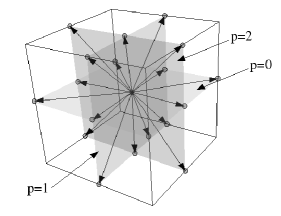
Figure 1: Cubic Lattice D3Q19 for modelling the electronic and ionic fluids. The arrows represent the velocity vectors $\vec{v}_{i}^{p}$ and $p$ indicates the plane of location.

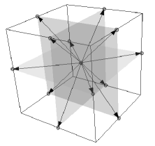
Figure 2: Cubic Lattice D3Q13 for modelling the electric field. The arrows represent the electric vectors $\vec{e}_{ij}^{p}$.

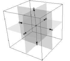
Figure 3: Cubic Lattice D3Q7 for simulating the magnetic field, the arrows indicate the magnetic vectors $\vec{b}_{ij}^{p}$.

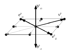
Figure 4: Index relationship between the velocity vectors and the electric and magnetic vectors.

For our 3D model, we use a cubic regular grid, with lattice constant $\delta x$$=$$\sqrt{2}c\delta t$ and $c$ is the light speed ($c$$\simeq$$3\times 10^{8}m/s$). There are 19 velocity vectors for the electronic and ionic fluids (figure 1), 13 vectors for the electric field (figure 2) and 7 vectors for the magnetic field (figure 3). The velocity vectors are denoted by $\vec{v}_{i}^{p}$, where $i=1,2,3,4,5,6$ indicates the direction and $p=0,1,2$ indicates the plane of location. Their components are

$$\vec{v}_{i}^{0}=c\sqrt{2}(\cos((2i-1)\pi/4),\sin((2i-1)\pi/4),0)\quad,$$ (3a)

$$\vec{v}_{i}^{1}=c\sqrt{2}(\cos((2i-1)\pi/4),0,\sin((2i-1)\pi/4))\quad,$$ (3b)

$$\vec{v}_{i}^{2}=c\sqrt{2}(0,\cos((2i-1)\pi/4),\sin((2i-1)\pi/4))\quad,$$ (3c)

for $i<5$, and

$$\vec{v}_{i}^{0}=c\sqrt{2}((-1)^{i},0,0)\quad,$$ (4a)

$$\vec{v}_{i}^{1}=c\sqrt{2}(0,(-1)^{i},0)\quad,$$ (4b)

$$\vec{v}_{i}^{2}=c\sqrt{2}(0,0,(-1)^{i})\quad,$$ (4c)

for $i\geq 5$. This makes 18 vectors. The missing one is the rest vector $\vec{v}_{0}$, with componets $(0,0,0)$.

The set of 13 electric field vectors, $\vec{e}_{ij}^{p}$, and 7 magnetic field vectors, $\vec{b}_{ij}^{p}$ are related with the velocity vectors as follows:

$$\vec{e}_{i0}^{p}=\frac{1}{2}\vec{v}_{(i-1)mod4}^{p}\quad,\quad\vec{e}_{i1}^{p}=\frac{1}{2}\vec{v}_{(i+1)mod4}^{p}\quad,$$ (5)

and

$$\vec{b}_{ij}^{p}=\frac{1}{2c^{2}}\vec{v}_{i}^{p}\times\vec{e}_{ij}^{p}\quad,$$ (6)

where the index $i$ takes the values $i$$=$$1,2,3,4$.

The distribution functions that describe the fluids, denoted by $f_{i}^{p(s)}$ and $f_{0}^{(s)}$, propagate with each velocity vector $\vec{v}_{i}^{p}$ and with the rest vector $\vec{v}_{0}$, respectively, and uses these vectors to compute the velocity fields for each fluid. Here, the index $s$ distinguishs between electronic ($s$$=$$0$) and ionic ($s$$=$$1$) fluids. Similarly, the distribution functions associated for the electromagnetic field are denoted by $f_{ij}^{p(2)}$ and $f_{0}^{(2)}$. They also propagate in the direction of the velocity vectors $\vec{v}_{i}^{p}$ and $\vec{v}_{0}$, but they use the electric and magnetic field vectors to compute those fields. Summarizing, The macroscopic variables are computed as follows:

$$\rho_{s}=f_{0}^{s}+\sum_{i,p}f_{i}^{p(s)}\quad,$$ (7a)

$$\rho_{s}\vec{V_{s}}=\sum_{i,p}f_{i}^{p(s)}\vec{v}_{i}^{p}\quad,$$ (7b)

$$\vec{E}=\sum_{i,j,p}f_{ij}^{p(2)}\vec{e}_{ij}^{p}\quad,$$ (7c)

$$\vec{B}=\sum_{i,j,p}f_{ij}^{p(2)}\vec{b}_{ij}^{p}\quad,$$ (7d)

$$\vec{J}=\sum_{s}\frac{q_{s}}{m_{s}}\rho_{s}\vec{V}_{s}\quad,$$ (7e)

$$\rho_{c}=\sum_{s}\frac{q_{s}}{m_{s}}\quad,$$ (7f)

where $\rho_{s}$ and $\vec{V}_{s}$ are the density and velocity of each fluid, and $m_{s}$ and $q_{s}$ are its particle mass and charge (here, $s$$=$$0$ represents electrons and $s$$=$$1$ represents ions, as before). In addition, $\vec{E}$ and $\vec{B}$ are the electric and magnetic fields, $\vec{J}$ is the total current density and $\rho_{c}$ is the total charge density.

For their evolution, we follow the proponsal of J.M. Buick and C.A. Greated for the lattice Boltzmann equations Buick and Greated (2000),

$${}\begin{aligned} f_{i}^{p(s)}(\vec{x}+\vec{v}_{i}^{p}\delta t,t+\delta t)-f_{i}^{p(s)}(\vec{x},t)=&\\ \Omega_{i}^{p(s)}(\vec{x},t)+&\frac{\kappa_{s}\delta t}{20c^{2}}(\vec{v}_{i}^{p}\cdot\vec{F}^{(s)}),\end{aligned}$$ (8)

$${}\begin{aligned} f_{ij}^{p(2)}(\vec{x}+\vec{v}_{i}^{p}\delta t,t+\delta t)-f_{ij}^{p(2)}(\vec{x},t)=&\\ \Omega_{ij}^{p(2)}(\vec{x},t)-&\frac{\kappa_{2}\mu_{0}\delta t}{8}(\vec{e}_{ij}^{p}\cdot\vec{J^{\prime}}),\end{aligned}$$ (9)

$${}f_{0}^{(K)}(\vec{x},t+\delta t)-f_{0}^{(K)}(\vec{x},t)=\Omega_{0}^{(K)}(\vec{x},t)\quad,$$ (10)

where $K=0,1,2$. The force vectors $\vec{F}^{(s)}$ in Eq.(8) are

$${}\begin{aligned} \vec{F}^{(s)}=&\frac{q_{s}}{m_{s}}\rho_{s}(\vec{E}+\vec{V}_{s}\times\vec{B})\\ &-\nu\rho_{s}(\vec{V}_{s}-\vec{V}_{(s+1)mod2})+\vec{F}^{(s)}_{0}\quad,\end{aligned}$$ (11)

where $\nu$ is the collision frequency of the plasma, $\vec{F}^{(s)}_{0}$ is any external force (for instance, a gravitational force) and the equilibrium density current vector $\vec{J^{\prime}}$ in Eq. (9) is defined by

$${}\vec{J^{\prime}}=\sum_{s}\frac{q_{s}}{m_{s}}\rho_{s}\biggl{(}\vec{V}_{s}+\frac{\lambda_{s}\tau_{s}\delta t\vec{F}^{(s)}}{\rho_{s}}\biggr{)}\quad.$$ (12)

The collision terms $\Omega_{ij}^{p(K)}$ and $\Omega_{0}^{(K)}$ are given by

$$\Omega_{i}^{p(s)}=-\frac{1}{\tau_{s}}(f_{i}^{p(s)}(\vec{x},t)-f_{i}^{p(s)\rm eq}(\vec{x},t))\quad,$$ (13a)

$$\Omega_{ij}^{p(2)}=-\frac{1}{\tau_{2}}(f_{ij}^{p(2)}(\vec{x},t)-f_{ij}^{p(2)\rm eq}(\vec{x},t))\quad,$$ (13b)

$$\Omega_{0}^{(K)}=-\frac{1}{\tau_{K}}(f_{0}^{(K)}(\vec{x},t)-f_{0}^{(K)\rm eq}(\vec{x},t))\quad,$$ (13c)

where $\tau_{K}$ is the relaxation time, $\kappa_{K}$$=$$\frac{2\tau_{K}-1}{2\tau_{K}}$ and $\lambda_{s}$$=$$\frac{1}{2\tau_{s}}$.

The equilibrium functions for the fluids, $f_{i}^{p(s)\rm eq}$ and $f_{0}^{(s)\rm eq}$ are

$$\begin{aligned} f_{i}^{p(s)\rm eq}(\vec{x},t)=&\omega_{i}\rho_{s}\biggl{[}3\xi_{s}\rho_{s}^{\gamma-1}+3(\vec{v}_{i}^{p}\cdot\vec{V^{\prime}}_{s})\biggr{.}\\ &\biggl{.}+\frac{9}{4c^{2}}(\vec{v}_{i}^{p}\cdot\vec{V^{\prime}}_{s})^{2}-\frac{3}{2}(\vec{V^{\prime}}_{s}^{2})\biggr{]}\quad,\end{aligned}$$ (14a)

$$f_{0}^{p(s)\rm eq}(\vec{x},t)=6\rho_{s}c^{2}\biggl{[}1-\frac{1}{4c^{2}}(4\xi_{s}\rho_{s}^{\gamma-1}+\vec{V^{\prime}}_{s}^{2})\biggr{]}\quad,$$ (14b)

where the weights $w_{i}$ are $w_{0}=\frac{1}{6c^{2}}$, $w_{1,2,3,4}=\frac{1}{72c^{2}}$, $w_{5,6}=\frac{1}{36c^{2}}$. In addition, $\xi_{s}$ is a constant that is fixed by the initial fluid temperature and density by means of the ideal gas law,

$${}\xi_{s}=\rho_{s(t=0)}^{1-\gamma}\frac{k}{m_{s}}T_{s(t=0)}\quad,$$ (15)

with polytropic index $\gamma$, and $k$ is the Boltzmann constant. The equilibrium velocity $\vec{V^{\prime}}_{s}$ is defined by

$${}\vec{V^{\prime}}_{s}=\vec{V}_{s}+\frac{\lambda_{s}\tau_{s}\delta t\vec{F}^{(s)}}{\rho_{s}}\quad.$$ (16)

For the electromagnetic field ($K=2$), we have

$$f_{ij}^{p(2)\rm eq}(\vec{x},t)=\frac{1}{8c^{2}}\vec{E^{\prime}}\cdot\vec{e}_{ij}^{p}+\frac{1}{8}\vec{B}\cdot\vec{b}_{ij}^{p}\quad,$$ (17a)

$$f_{0}^{(2)\rm eq}(\vec{x},t)=0\quad,$$ (17b)

where the equilibrium electric field is

$$\vec{E^{\prime}}=\vec{E}-(\mu_{0}c^{2}\lambda_{2}\tau_{2}\delta t)\vec{J^{\prime}}\quad,$$ (18a)

and $\lambda_{2}$$=$$\frac{1}{2\tau_{2}}$, as before.

The proof that this lattice Boltzmann model, via a Chapman-Enskog expansion, recovers the equations of the two-fluids theory for a plasma composed by electrons and ions is shown in Appendix A. The model let us to consider either compressible and non-viscous fluids or incompressible and viscous fluids. The first ones are governed by the continuity equation

$${}\vec{\nabla}\cdot(\rho_{s}{\vec{V}^{\prime}}_{s})+\frac{\partial\rho_{s}}{\partial t}=0\quad,$$ (19)

the Navier-Stokes equation,

$${}\begin{aligned} \rho_{s}\biggl{(}\frac{\partial\vec{V^{\prime}}_{S}}{\partial t}+&(\vec{V^{\prime}}\cdot\vec{\nabla})\vec{V^{\prime}}_{s}\biggr{)}=\\ -&\vec{\nabla}P_{s}+\frac{q_{s}}{m_{s}}\rho_{s}(\vec{E}+\vec{V^{\prime}}_{s}\times\vec{B})\\ -&\nu\rho_{s}(\vec{V^{\prime}}_{s}-\vec{V^{\prime}}_{(s+1)mod2})+\vec{F}_{0}\quad.\end{aligned}$$ (20)

the state equation,

$${}P_{s}=\xi_{s}\rho_{s}^{\gamma}\quad,$$ (21)

where $P_{s}$ is the fluid pressure, and the Maxwell equations. The second ones are governed by the state equation (21), Maxwell equations, the continuity equation

$${}\vec{\nabla}\cdot\vec{V}^{\prime}_{s}=0\quad$$ (22)

and the Navier-Stokes equation for an incompressible and viscous fluid,

$${}\begin{aligned} \rho_{s}\biggl{(}\frac{\partial\vec{V^{\prime}}_{s}}{\partial t}&+(\vec{V^{\prime}}\cdot\vec{\nabla})\vec{V^{\prime}}_{s}\biggr{)}=\\ &-\vec{\nabla}P_{s}+\frac{q_{s}}{m_{s}}\rho_{s}(\vec{E}+\vec{V^{\prime}}_{s}\times\vec{B})\\ &-\nu\rho_{s}(\vec{V^{\prime}}_{s}-\vec{V^{\prime}}_{(s+1)mod2})\\ &+\vec{F}_{0}+\eta_{s}\rho_{s}\vec{\nabla}^{2}\vec{V^{\prime}}_{s}\quad.\end{aligned}$$ (23)

where the kinematic viscosity is $\eta_{s}$$=$$\frac{2}{3}(\tau_{s}-1/2)c^{2}\delta t$.

III Simulation of a 2D Hartmann Flow

In the MHD limit, the two-fluid theory becomes the MHD (one fluid) theory, which is represented by the following equations: the continuity of mass,

$${}\vec{\nabla}\cdot(\rho\vec{V})+\frac{\partial\rho}{\partial t}=0\quad,$$ (24)

the Navier-Stokes equation,

$${}\rho\biggl{(}\frac{\partial}{\partial t}+\vec{V}\cdot\vec{\nabla}\biggr{)}\vec{V}=-\vec{\nabla}P+\vec{J}\times\vec{B}+\eta\vec{\nabla}^{2}\vec{V}+\vec{F}_{0},$$ (25)

the magnetic field equation,

$${}\frac{\partial\vec{B}}{\partial t}=\vec{\nabla}\times(\vec{V}\times\vec{B})+\eta_{m}\vec{\nabla}^{2}\vec{B}\quad,$$ (26)

and the state equation,

$${}P=\xi_{s}\rho^{\gamma}\quad,$$ (27)

where $\rho$ is the total mass density, $\vec{V}$ is the total velocity field and $\eta_{m}$$=$$\frac{1}{\mu_{0}\sigma_{0}}$ is the magnetic viscosity.

For the Hartmann flow Schaffenberger and Hanslmeier (2002); David (1966), we consider a fluid in isotermal equilibrium ($\gamma=1$) at low temperature (a small $\xi_{s}$ value), incompressible and viscous. The fluid moves in the $x$ direction between two walls at rest at $y$$=$$-L$ and $y$$=$$-L$. There is a constant magnetic field in the $y$ direction, with intensity $B_{0}$, and a constant external force $F$$=$$\rho g$ in the $x$ direction to drag the fluid Schaffenberger and Hanslmeier (2002). So, the velocity and magnetic fields take the forms $\vec{V}$$=$$(V_{x}(y),0,0)$ and $\vec{B}=(B_{x}(y),B_{0},0)$, respectively. By replacing these expressions in equations (25) and (26), one finds the following solutions for the velocity and magnetic fields Schaffenberger and Hanslmeier (2002):

$$V_{x}(y)=\sqrt{\frac{\rho\eta_{m}}{\eta}}\frac{gL}{B_{0}}\cosh(H)\biggl{[}1-\frac{\cosh(Hy/L)}{\cosh(H)}\biggr{]}\quad,$$ (28a)

$$B_{x}(y)=\frac{\rho gL}{B_{0}}\biggl{[}\frac{\sinh(Hy/L)}{\sinh(H)}-\frac{y}{L}\biggr{]}\quad,$$ (28b)

where $H$$=$$\frac{B_{0}L}{\sqrt{\rho\eta\eta_{m}}}$ is the Hartmann number and $-L\leq y\leq L$.

For the simulation, we use a single row of $80$ cells in the $y$ direction, with periodic boundary conditions in both $x$ and $z$ directions. The initial conditions for the density functions are obtained from the equilibrium expressions (14) and (17) with the values $\vec{V}_{s}$$=$$0$, $\rho_{s}$$=$$m_{s}n_{s}$, $\vec{E}$$=$$0$, $\vec{B}$$=$$(0,B_{0},0)$ and $\vec{F}^{(s)}_{0}$$=$$(\rho_{s}g,0,0)$. In addition, the constant values are $\gamma$$=$$1$, $\xi_{s}$$=$$3\times 10^{-6}$, $\mu_{0}$$=$$1.0$, $c$$=$$1$, $\nu$$=$$100$, $\tau_{s}$$=$$1.0$, $\tau_{2}$$=$$0.5$, $m_{0}$$=$$1.0\times 10^{-19}$, $m_{1}$$=$$1820m_{0}$, and $n_{0}$$=$$n_{1}$$=$$1.0\times 10^{19}$ particles per unit volume. For the $y$ direction, we assume as boundary conditions at the walls that the equilibrium density functions for the time evolution (Eq. (14) and (17)) are always the same from the initial conditions (including $\vec{V}_{s}$$=$$0$, i.e. non-conducting walls). The system evolves until a steady state is reached. We ran simulations for Hartmann numbers $H$$=$$5$, $13$ and $26$, and the magnetic field $B_{0}$ was chosen to obtain these Hartmann numbers.

Figure 5 shows the velocity profiles and figure 6 shows the magnetic field profiles for the three cases. The solid lines are the analytic solutions (Eq.(28)). The simulation results are in excellent agreement with the analytical solutions. This result say us that (at least for the MHD limit) our LB models works properly.

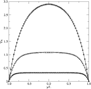
Figure 5: Velocity profile Vx vs. y/L for different Hartmann numbers: H=6.0 (circles), H=13.0 (squares) and H=26.0 (diamonds). The solid lines are the analytical results.

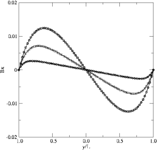
Figure 6: Magnetic field intensity Bx vs. y/L for different Hartmann numbers: H=6.0 (circles), H=13.0 (squares) and H=26.0 (diamonds). The solid lines are the analytical results.

IV Application to Magnetic Reconnection

IV.1 Dynamics of the magnetic reconnection process

In order to simulate the magnetic reconnection in the magnetotail, we chose the initial equilibrium condition proposed by Harris Harris (1962); J. et al. (1975) for the current sheet, plus a magnetic dipole field, ortogonal to the sheet. For this simulation we assume that the fluids are non-viscous and compressible.

The current sheet lies on the x-y plane, and its magnetic field is described by the vector potential $\vec{A}$$=$$(0,A_{y},0)$, with

$${}A_{y}(x,z)=LB_{0}\ln{\cosh[v(x)(z/L)]/v(x)}\quad,$$ (29)

where the effective thickness of the current sheet is given by $L/v(x)$, and the asymptotic strength, $B_{0}$, is the value of $B_{x}$ in the limit $z\to\infty$, divided by $v(x)$. The function $v(x)$ is an arbitrary slowly-varying function. We choose for $v(x)$ the quasi-parabolic function proposed by Pritchett and Coroniti (2001); Lembège and Pellat (1982),

$${}v(x)=\exp(-\epsilon x/L)\quad,$$ (30)

where the parameter $\epsilon$ is much smaller than one and determines the strength of the z-component of the magnetic field. We took $\epsilon$$=$$0.1$ for the simulation. The initial density is the one proposed by Harris,

$${}n_{s}(x,z)=n_{b}+n_{c}v^{2}(x)\cosh^{-2}[v(x)(z/L)]\quad,$$ (31)

where $n_{b}$ is the background density and $n_{b}+n_{c}$ is the maximal density.

The magnetic dipole is set at position $x_{0}$ with momentum $M$ and oriented in the $z$ direction. It generates a magnetic field given by

$$B_{x}(x,z)= \frac{3M(x-x_{0})z}{((x-x_{0})^{2}+z^{2})^{\frac{5}{2}}}\quad,$$ (32)

$$B_{y}(x,z)= 0\quad,$$

$$B_{z}(x,z)= \frac{M(2z^{2}-(x-x_{0})^{2})}{((x-x_{0})^{2}+z^{2})^{\frac{5}{2}}}\quad.$$

The lattice constant $\delta x$ is chosen as one seventh of the ion inertial length, $\delta x$$=$$\frac{1}{7}c/\omega_{1}$, where $\omega_{1}$ is the ion plasma frequency, $\omega_{1}$$=$$\sqrt{\frac{q_{1}^{2}n_{1}}{\epsilon_{0}m_{1}}}$, with $n_{1}$$=$$10^{5}$ particles per cubic meter for the magnetotail Runov et al. (2005a) and $m_{1}$ the proton mass. That gives $\delta x$$\simeq$$103$km. Since the current sheet in the magnetotail can be assumed around $3000$km width Runov et al. (2005a, b), we chose $L$$=$$2c/\omega_{1}$. For the position of the magnetic dipole, we took $x_{0}$$=$$22.7c/\omega_{1}$ and for the dipole momentum, $M$$=$$3\times 10^{12}$. The grid is an array of $100$$\times$$100$ cells on the x-z plane with periodic boundary conditions in the $y$ direction and free boundary conditions for the fields in the other directions (each boundary cell copies the density functions of its first neighbohr in ortogonal direction to the boundary at each time step). Thus, the simulation region is a square of $14.26c/\omega_{1}$ length (around $10300$km). For this simulation we took $m_{0}$$=$$m_{1}/100$ (i.e. an electron mass 20 times larger than the real one) in order to obtain numerical stability, but it has been shown Hesse et al. (1999) that this point does not qualitatively change the physical results. The temperature ratio is chosen to be $T_{0}/T_{1}$$=$$0.2$, acording to observational results Asano et al. (2004). For this simulation, we took $n_{c}$$=$$5n_{b}$ and $n_{b}$$=$$0.17n_{1}$.

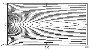
Figure 7: Magnetic field lines in the magnetic reconnection process at t=0 (initial conditions)

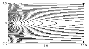
Figure 8: Evolution for the Magnetic field lines in the magnetic reconnection process, at $t=3/\Omega_{1}$

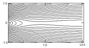
Figure 9: Evolution for the Magnetic field lines in the magnetic reconnection process, at $t=15/\Omega_{1}$

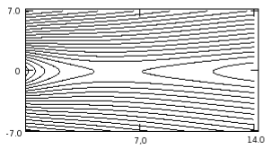
Figure 10: Evolution for the Magnetic field lines in the magnetic reconnection process, at $t=20/\Omega_{1}$

Figures 7, 8, 9 and 10 show the evolution of the magnetic field lines in the magnetic reconnection process. This appears in a natural way, without the a priori introduction of any resistive region. The factor $\Omega_{1}$ is the ionic cyclotron frequency, $\Omega_{1}=q_{1}B_{0}/m_{1}$. This result tell us that the model can actually simulate the magnetic reconnection. This simulation took 1h in a Pentium IV PC of 2.8GHz, i.e. it is really fast.

IV.2 Reconnection rates

To compute real reconnection rates we performed a similar simulation to the one before, but with the actual ratio between electronic and ionic masses ($m_{1}$$=1820m_{0}$). This choice bring us to take a shorter time steps ($\delta t$$=$$3.76\times 10^{-5}$s) and smaller cells ($\delta x$$=$$15.95$km) in order to reproduce with accuracy the electron moves. The LB array is $200$$\times$$100$ cells (larger in direction x), for a total simulation region of $3190$km in x and $1595$km in z. Since the region is smaller than before, $v(x)$$=$$1$ is a good approximation on the entire region. The simulation constants are $L$$=$$1595$km Runov et al. (2005a) and $B_{0}$$=$$10.0$$nT$ Runov et al. (2005b). The densities in Eq.(31) are $n_{b}$$=$$0$ and $n_{c}$$=$$10^{5}$$m^{-3}$ Runov et al. (2005a), the electronic temperature is chosen as $T_{0}$$=$$5.8$$MK$ and the ionic one as $T_{1}$$=$$23.2$$MK$ Asano et al. (2004). All these are observational data. The electronic mass is taken $m_{0}$$=$$9.11\times 10^{-31}$kg and the ionic mass is $m_{1}$$=$$1.67\times 10^{-27}$kg. All other constants of our LB model take their standard values in IS units.

The initial configuration of the magnetic field is shown in figure 11 and the same field after $t$$=$$1.92ms$ is shown in figure 12. The reconnection rate we obtain from this simulation is $R$$=$$0.109$, which is in good agreement with the experimental observations around $R$$\sim$$0.1$ Xiao et al. (2005). This simulation took just 5 minutes in a Pentium IV PC of 2.8GHz.

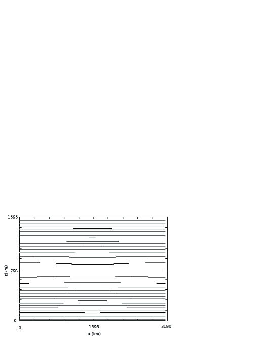
Figure 11: Magnetic field lines in the magnetic reconnection process at t=0 (initial conditions)

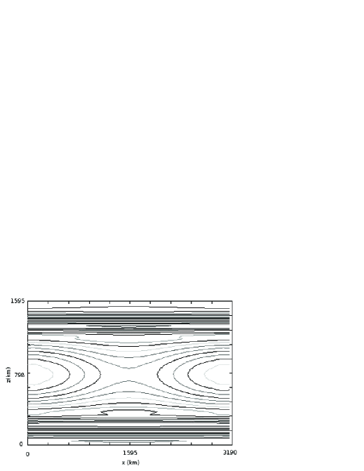
Figure 12: Evolution for the Magnetic field lines in the magnetic reconnection process, at $t=1.92ms$

V Conclusion

In this paper we introduce a 3D lattice Boltzmann model for simulating plasmas, which is able to simulate magnetic reconnection without any previous assumption of a resistive region or an anomalous resistivity. The model simulates the plasma as two fluids (one electronic and one ionic) with an interaction term, and reproduces in the continuous limit the equations of the two-fluids theory and, therefore, the MHD-Hall equations. This model can simulate either conducting and viscous fluids in the incompressible limit or non-viscous compressible fluids, and sucessfully reproduces both the Hartmann flow and the magnetic reconnection in the magnetotail. The reconnection rate we obtain with this model is $R$$=$$0.109$, which is in excellent agreement with observations.

Since this method includes both electric and magnetic fields, plus the density and velocity fields for each fluid, it gives much more information on the details of the plasma physics. Moreover, this opens the door to much more sophisticated boundary conditions, like conductive walls or electromagnetic waves in plasmas. This is an advantage upon other magnetohydrodynamic LB models. Furthermore, it is 3D, so many interest phenomena can be investigated here. The model does not require large computational resorces. It just takes between 5 minutes and 1h in a Pentium IV PC of 2.8GHz and uses around 100MB of RAM.

The model introduces the forces at first order in time, but this is not a problem for weak electromagnetic fields and low resistive plasmas. If this is not the case, it is possible to modify the charge/mass ratio, but this changes the MHD-Hall equations and slows the evolution of the electromagnetic fields. Another way to increase the numerical stability consists of modifying the model to reproduce the two fluids in a different way: by defining density functions for the sum, $f_{i}^{p(0)}+f_{i}^{p(1)}$, and the difference, $\frac{q_{0}}{m_{0}}f_{i}^{p(0)}+\frac{q_{1}}{m_{1}}f_{i}^{p(1)}$ of the two fluids. It is also possible to develop a LB model with 13 velocity vectors for the fluids, as proposed by Cowling (1968). These are promisory paths of future work.

Hereby we have introduced a 3D lattice Botzmann model that reproduces the two-fluid theory and includes in a natural way many aspects of interest in plasma physics, like electric fields and magnetic reconnection. It has been shown in this work that this model can actually be used to investigate real astrophysical problems. We hope that this LB model will contribute to the study of plasma physics in many interesting phenomena.

Appendix A Chapman-Enskog Expansion

The Boltzmann equations for each fluid, Eq. (8), (9) and (10), determine the system evolution. This evolution rule gives in the continuum limit the macroscopic differential equation that the system satisfies. This is known as the Chapman-Enskog expansion. To develop it, we start by taking the Taylor expansion of these equations until second order in spatial and temporal $(\delta\vec{x},\delta t)$ variables,

$${}\begin{aligned} &\vec{v}_{i}^{p}\cdot\vec{\nabla}f_{i}^{p(s)}\delta t+\frac{1}{2}\sum_{\alpha,\beta}\frac{\partial^{2}f_{i}^{p(s)}}{\partial x_{\alpha}\partial x_{\beta}}(v_{i\alpha}^{p}v_{i\beta}^{p})\delta t^{2}\\ &+\frac{\partial f_{i}^{p(s)}}{\partial t}\delta t+\frac{\partial}{\partial t}\vec{v}_{i}^{p}\cdot\vec{\nabla}f_{i}^{p(s)}\delta t^{2}\\ &+\frac{1}{2}\frac{\partial^{2}f_{i}^{p(s)}}{\partial t^{2}}\delta t^{2}=-\frac{1}{\tau_{s}}(f_{i}^{p(s)}-f_{i}^{p(s)\rm eq})\\ &+\frac{\kappa_{s}\delta t}{20c^{2}}(\vec{v}_{i}^{p}\cdot\vec{F}^{(s)})\quad,\end{aligned}$$ (33)

$${}\begin{aligned} &\vec{v}_{i}^{p}\cdot\vec{\nabla}f_{ij}^{p(2)}\delta t+\frac{1}{2}\sum_{\alpha,\beta}\frac{\partial^{2}f_{ij}^{p(2)}}{\partial x_{\alpha}\partial x_{\beta}}(v_{i\alpha}^{p}v_{i\beta}^{p})\delta t^{2}\\ &+\frac{\partial f_{ij}^{p(2)}}{\partial t}\delta t+\frac{\partial}{\partial t}\vec{v}_{i}^{p}\cdot\vec{\nabla}f_{ij}^{p(2)}\delta t^{2}\\ &+\frac{1}{2}\frac{\partial^{2}f_{i}^{p(s)}}{\partial t^{2}}\delta t^{2}=-\frac{1}{\tau_{2}}(f_{ij}^{p(2)}-f_{ij}^{p(2)\rm eq})\\ &-\frac{\kappa_{2}\mu_{0}\delta t}{8}(\vec{e}_{ij}^{p}\cdot\vec{J^{\prime}})\quad,\end{aligned}$$ (34)

$${}\begin{aligned} \frac{\partial f_{0}^{(K)}}{\partial t}\delta t+\frac{1}{2}\frac{\partial^{2}f_{0}^{(K)}}{\partial t^{2}}\delta t^{2}=-\frac{1}{\tau_{K}}(f_{0}^{(K)}-f_{0}^{(K)\rm eq})\quad.\end{aligned}$$ (35)

where $\alpha,\beta$$=$$x,y,z$ denotes the components in $x$, $y$ and $z$ directions.

Next, we expand the distribution functions and the spatial and time derivatives in a power series on a small parameter, $\epsilon$,

$$f_{ij}^{p(2)}=f_{ij}^{p(2)(0)}+\epsilon f_{ij}^{p(2)(1)}+\epsilon^{2}f_{ij}^{p(2)(2)}+...\quad,$$ (36)

$$f_{i}^{p(s)}=f_{i}^{p(s)(0)}+\epsilon f_{i}^{p(s)(1)}+\epsilon^{2}f_{i}^{p(s)(2)}+...\quad,$$ (37)

$$\frac{\partial}{\partial t}=\epsilon\frac{\partial}{\partial t_{1}}+\epsilon^{2}\frac{\partial}{\partial t_{2}}+...\quad,$$ (38)

$$\frac{\partial}{\partial x_{\alpha}}=\epsilon\frac{\partial}{\partial x_{\alpha 1}}+...\quad.$$ (39)

It is assumed that only the 0th order terms in $\epsilon$ of the distribution functions contribute to the macroscopic variables. So, for $n>0$ we have

$$f_{0}^{s(n)}+\sum_{i,p}f_{i}^{p(s)(n)}=0\quad,$$ (40a)

$$\sum_{i,p}f_{i}^{p(s)(n)}\vec{v}_{i}^{p}=0\quad,$$ (40b)

$$\sum_{i,j,p}f_{ij}^{p(2)(n)}\vec{e}_{ij}^{p}=0\quad,$$ (40c)

$$\sum_{i,j,p}f_{ij}^{p(2)(n)}\vec{b}_{ij}^{p}=0\quad.$$ (40d)

The external forces $\vec{F}^{(s)}$ and the current density $\vec{J^{\prime}}$ are of order $\epsilon$ Buick and Greated (2000), so we can write $\vec{F}^{(s)}$$=$$\epsilon\vec{F}^{(s)}_{1}$ and $\vec{J^{\prime}}$$=$$\epsilon\vec{J^{\prime}}_{1}$. Because $f_{i}^{p(s)\rm eq}$ and $f_{ij}^{p(2)\rm eq}$ are now functions of $\vec{F}^{(s)}$ and $\vec{J^{\prime}}$, we need to develop a Chapman-Enskog expansion of the equilibrium function, too:

$$f_{i}^{p(s)\rm eq}=f_{i}^{p(s)(0)\rm eq}+\epsilon f_{i}^{p(s)(1)\rm eq}+\epsilon^{2}f_{i}^{p(s)(2)\rm eq}\quad,$$ (41)

$$f_{ij}^{p(2)\rm eq}=f_{ij}^{p(2)(0)\rm eq}+\epsilon f_{ij}^{p(2)(1)\rm eq}+\epsilon^{2}f_{ij}^{p(2)(2)\rm eq}\quad.$$ (42)

Thus, by replacing these results into Eqs.(33), (34) and (35), we obtain at zeroth order of $\epsilon$

$$f_{i}^{p(s)(0)\rm eq}=f_{i}^{p(s)(0)}\quad,$$ (43a)

$$f_{0}^{(K)(0)\rm eq}=f_{0}^{(K)(0)}\quad,$$ (43b)

$$f_{ij}^{p(2)(0)\rm eq}=f_{ij}^{p(2)(0)}\quad.$$ (43c)

For the first order terms in $\epsilon$ of the distribution functions we obtain

$${}\begin{aligned} \vec{v}_{i}^{p}\cdot\vec{\nabla}_{1}f_{i}^{p(s)(0)}\delta t&+\frac{\partial f_{i}^{p(s)(0)}}{\partial t_{1}}\delta t=\\ &-\frac{1}{\tau_{s}}(f_{i}^{p(s)(1)}-f_{i}^{p(s)(1)\rm eq})\\ &+\frac{\kappa_{s}\delta t}{20c^{2}}(\vec{v}_{i}^{p}\cdot\vec{F}^{(s)}_{1})\quad,\end{aligned}$$ (44a)

$${}\begin{aligned} \vec{v}_{i}^{p}\cdot\vec{\nabla}_{1}f_{ij}^{p(2)(0)}\delta t&+\frac{\partial f_{ij}^{p(2)(0)}}{\partial t_{1}}\delta t=\\ &-\frac{1}{\tau_{2}}(f_{ij}^{p(2)(1)}-f_{ij}^{p(2)(1)\rm eq})\\ &-\frac{\kappa_{2}\mu_{0}\delta t}{8}(\vec{e}_{ij}^{p}\cdot\vec{J^{\prime}}_{1})\quad,\end{aligned}$$ (44b)

$${}\begin{aligned} \frac{\partial f_{0}^{(K)(0)}}{\partial t_{1}}\delta t=-\frac{1}{\tau_{K}}(f_{0}^{(K)(1)}-f_{0}^{(K)(1)\rm eq})\quad,\end{aligned}$$ (44c)

and for the second order terms in $\epsilon$ we have

$${}\begin{aligned} &\biggl{(}1-\frac{1}{2\tau_{s}}\biggr{)}\biggl{(}\vec{v}_{i}^{p}\cdot\vec{\nabla}_{1}+\frac{\partial}{\partial t_{1}}\biggr{)}f_{i}^{p(s)(1)}\delta t\\ &+\frac{\partial f_{i}^{p(s)(0)}}{\partial t_{2}}\delta t+\frac{\delta t}{2\tau_{s}}\biggl{(}\vec{v}_{i}^{p}\cdot\vec{\nabla}_{1}+\frac{\partial}{\partial t_{1}}\biggr{)}f_{i}^{p(s)(1)\rm eq}\\ &+\frac{\kappa_{s}\delta t}{40c^{2}}\biggl{(}\vec{v}_{i}^{p}\cdot\vec{\nabla}_{1}+\frac{\partial}{\partial t_{1}}\biggr{)}(\vec{v}_{i}^{p}\cdot\vec{F}^{(s)}_{1})=\\ &-\frac{1}{\tau_{s}}(f_{i}^{p(s)(2)}-f_{i}^{p(s)(2)\rm eq})\quad,\end{aligned}$$ (45a)

$${}\begin{aligned} &\biggl{(}1-\frac{1}{2\tau_{2}}\biggr{)}\biggl{(}\vec{v}_{i}^{p}\cdot\vec{\nabla}_{1}+\frac{\partial}{\partial t_{1}}\biggr{)}f_{ij}^{p(2)(1)}\delta t\\ &+\frac{\partial f_{ij}^{p(2)(0)}}{\partial t_{2}}\delta t+\frac{\delta t}{2\tau_{2}}\biggl{(}\vec{v}_{i}^{p}\cdot\vec{\nabla}_{1}+\frac{\partial}{\partial t_{1}}\biggr{)}f_{ij}^{p(2)(1)\rm eq}\\ &+\frac{\mu_{0}\kappa_{2}\delta t}{16c^{2}}\biggl{(}\vec{v}_{i}^{p}\cdot\vec{\nabla}_{1}+\frac{\partial}{\partial t_{1}}\biggr{)}(\vec{e}_{ij}^{p}\cdot\vec{J^{\prime}}_{1})=\\ &-\frac{1}{\tau_{2}}(f_{ij}^{p(2)(2)}-f_{ij}^{p(2)(2)\rm eq})\quad,\end{aligned}$$ (45b)

$${}\frac{\partial f_{0}^{(K)(0)}}{\partial t_{1}}\delta t=-\frac{1}{\tau_{K}}(f_{0}^{(K)(1)}-f_{0}^{(K)(1)\rm eq})\quad.$$ (45c)

The terms of order one and two for the equilibrium functions of the fluids are obtained by replacing Eq. (16) into Eq.(14). That gives

$$\begin{aligned} f_{i}^{p(s)\rm eq}(\vec{x},t)&=\omega_{i}\rho_{s}\biggl{[}3\xi_{s}\rho_{s}^{\gamma-1}+\biggr{.}\\ &3\biggl{(}\vec{v}_{i}^{p}\cdot\biggl{(}\vec{V}_{s}+\frac{\epsilon\lambda_{s}\tau_{s}\delta t\vec{F}^{(s)}_{1}}{\rho_{s}}\biggr{)}\biggr{)}+\\ &\frac{9}{4c^{2}}\biggl{(}\vec{v}_{i}^{p}\cdot\biggl{(}\vec{V}_{s}+\frac{\epsilon\lambda_{s}\tau_{s}\delta t\vec{F}^{(s)}_{1}}{\rho_{s}}\biggr{)}\biggr{)}^{2}\\ &-\biggl{.}\frac{3}{2}\biggl{(}\vec{V}_{s}+\frac{\epsilon\lambda_{s}\tau_{s}\delta t\vec{F}^{(s)}_{1}}{\rho_{s}}\biggr{)}^{2}\biggr{]}\quad,\end{aligned}$$ (46a)

$$\begin{aligned} f_{0}^{p(s)\rm eq}(\vec{x},t)=&6\rho_{s}c^{2}\biggl{(}1-\frac{1}{4c^{2}}\biggl{(}4\xi_{s}\rho_{s}^{\gamma-1}+\\ &\biggl{(}\vec{V}_{s}+\frac{\epsilon\lambda_{s}\tau_{s}\delta t\vec{F}^{(s)}_{1}}{\rho_{s}}\biggr{)}^{2}\biggr{)}\biggr{)}\quad.\end{aligned}$$ (46b)

From these equations we can obtain

$$\begin{aligned} f_{i}^{p(s)(0)\rm eq}(\vec{x},t)&=\omega_{i}\rho_{s}\biggl{[}3\xi_{s}\rho_{s}^{\gamma-1}+3(\vec{v}_{i}^{p}\cdot\vec{V}_{s})\biggr{.}\\ \biggl{.}&+\frac{9}{4c^{2}}(\vec{v}_{i}^{p}\cdot\vec{V}_{s})^{2}-\frac{3}{2}(\vec{V}_{s})^{2}\biggr{]}\quad,\end{aligned}$$ (47a)

$$\begin{aligned} f_{i}^{p(s)(1)\rm eq}(\vec{x},t)&=\omega_{i}\delta t\biggl{[}3\lambda_{s}\tau_{s}(\vec{v}_{i}^{p}\cdot\vec{F}^{(s)}_{1})\biggr{.}\\ &+\frac{9\lambda_{s}\tau_{s}}{2c^{2}}(\vec{v}_{i}^{p}\cdot\vec{V}_{s})(\vec{v}_{i}^{p}\cdot\vec{F}^{(s)}_{1})\\ &-\biggl{.}3\lambda_{s}\tau_{s}(\vec{V}_{s}\cdot\vec{F}^{(s)}_{1})\biggr{]}\quad,\end{aligned}$$ (47b)

$$\begin{aligned} f_{i}^{p(s)(2)\rm eq}(\vec{x},t)=\frac{\omega_{i}\delta t^{2}}{\rho_{s}}\biggl{[}\frac{9}{4c^{2}}\lambda^{2}_{s}\tau^{2}_{s}(\vec{v}_{i}^{p}\cdot\vec{F}^{(s)}_{1})^{2}\biggr{.}\\ \biggl{.}-\frac{3}{2}\lambda^{2}_{s}\tau^{2}_{s}(\vec{F}^{(s)}_{1})^{2}\biggr{]}\quad,\end{aligned}$$ (47c)

and

$$\begin{aligned} f_{0}^{p(s)(0)\rm eq}&(\vec{x},t)=\\ &6\rho_{s}c^{2}\biggl{(}1-\frac{1}{4c^{2}}(4\xi_{s}\rho_{s}^{\gamma-1}+(\vec{V}_{s})^{2})\biggr{)},\end{aligned}$$ (47d)

$$\begin{aligned} f_{0}^{p(s)(1)\rm eq}(\vec{x},t)=-6\delta tc^{2}\biggl{(}\frac{\lambda_{s}\tau_{s}}{2c^{2}}(\vec{V}_{s}\cdot\vec{F}^{(s)}_{1})\biggr{)},\end{aligned}$$ (47e)

$$\begin{aligned} f_{0}^{p(s)(2)\rm eq}&(\vec{x},t)=\\ &-\frac{6\delta t^{2}c^{2}}{\rho_{s}}\biggl{(}\frac{\lambda^{2}_{s}\tau^{2}_{s}}{4c^{2}}(\vec{F}^{(s)}_{1}\cdot\vec{F}^{(s)}_{1})\biggr{)},\end{aligned}$$ (47f)

The same process can be used to determine the terms of order one and two for the equilibrium functions of the electromagnetic fields. Replacing Eq. (18) into Eq. (17) and grouping, we have

$$f_{ij}^{p(2)(0)\rm eq}(\vec{x},t)=\frac{1}{8c^{2}}\vec{E}\cdot e_{ij}^{p}+\frac{1}{8}\vec{B}\cdot b_{ij}^{p}\quad,$$ (48a)

$$f_{ij}^{p(2)(1)\rm eq}(\vec{x},t)=-\frac{\epsilon\mu_{0}\lambda_{2}\tau_{2}\delta t}{8}\vec{J^{\prime}}_{1}\cdot e_{ij}^{p}\quad,$$ (48b)

$$f_{ij}^{p(2)(2)\rm eq}(\vec{x},t)=0\quad.$$ (48c)

Now, we are ready to determine the equation that the model satisfies in the continuum limit. First, let us consider non-viscous compressible fluids, that is $\tau_{s}$$=$$\frac{1}{2}$. By summing up Eq. (44a) over $i$ and $p$, and by taking into account Eqs. (44c), (7), (47) and (40), we get

$${}\vec{\nabla}\cdot(\rho_{s}\vec{V}_{s})+\frac{\partial\rho_{s}}{\partial t_{1}}=0\quad.$$ (49)

By summing up Eq. (45a) in the same way, we obtain

$${}\vec{\nabla}\cdot\biggl{(}\frac{\lambda_{s}+\kappa_{s}}{2}\delta t\vec{F}^{(s)}_{1}\biggr{)}+\frac{\partial\rho_{s}}{\partial t_{2}}=0\quad.$$ (50)

Now, we can add these two equations to obtain

$${}\vec{\nabla}\cdot\biggl{(}\rho_{s}\vec{V}_{s}+\frac{\lambda_{s}+\kappa_{s}}{2}\delta t\vec{F}^{(s)}_{1}\biggr{)}+\frac{\partial\rho_{s}}{\partial t_{1}}=0\quad.$$ (51)

Next, following Buick and Greated Buick and Greated (2000), we do $\lambda_{s}$$=$$\frac{1}{2\tau_{s}}$, $\kappa_{s}$$=$$\frac{2\tau_{s}-1}{2\tau_{s}}$ and, by taking into account Eq. (16), we arrive to the continuity equation

$${}\vec{\nabla}\cdot(\rho_{s}{\vec{V}^{\prime}}_{s})+\frac{\partial\rho_{s}}{\partial t}=0\quad.$$ (52)

By multiplying Eq. (44a) by $\vec{v}_{i}^{p}$ and summing up over $i$ and $p$, we get

$${}\frac{\partial}{\partial x_{\beta}}(\rho_{s}V_{s\alpha}V_{s\beta})+\frac{\partial(\xi_{s}\rho_{s}^{\gamma})}{\partial x_{\alpha}}+\frac{\partial(\rho_{s}V_{s\alpha})}{\partial t_{1}}=F_{1\alpha}^{(s)}.$$ (53)

In a similar way, by multiplying Eq. (45a) by $\vec{v}_{i}^{p}$ and summing up over $i$ and $p$, we obtain

$${}\frac{\partial(\rho_{s}V_{s\alpha})}{\partial t_{2}}+\frac{\delta t}{2}\frac{\partial}{\partial x_{\beta}}(F^{(s)}_{1\beta}V_{s\alpha}+F^{(s)}_{1\alpha}V_{s\beta})$$

$$+\frac{\delta t}{2}\frac{\partial F_{1\alpha}^{(s)}}{\partial t_{1}}=0\quad.$$ (54)

Now, we can add these two equations, and by replacing Eq. (16), we get (up to second order in $\epsilon$)

$${}\frac{\partial(\rho_{s}V^{\prime}_{s\alpha})}{\partial t}+\frac{\partial}{\partial x_{\beta}}(\rho_{s}{V^{\prime}}_{s\alpha}{V^{\prime}}_{s\beta})=-\frac{\partial P_{s}}{\partial x_{\alpha}}+F_{1\alpha}^{(s)}\quad.$$ (55)

This is the Navier-Stokes equation for non-viscous compressible fluids, with state equation $P_{s}$$=$$\xi_{s}\rho_{s}^{\gamma}$. In our model, the force $F_{\alpha}^{(s)}$ is taken at first order in $\epsilon$. With this approximation, Eq.(11) gives $F_{1\alpha}^{(s)}(\vec{V}_{s})$$=$$F_{1\alpha}^{(s)}(\vec{V^{\prime}}_{s})$, and the Navier-Stokes equation is

$${}\begin{aligned} \frac{\partial(\rho_{s}V^{\prime}_{s\alpha})}{\partial t}&+\frac{\partial}{\partial x_{\beta}}(\rho_{s}{V^{\prime}}_{s\alpha}{V^{\prime}}_{s\beta})=\\ &-\frac{\partial P_{s}}{\partial x_{\alpha}}+\biggl{(}\frac{q_{s}}{m_{s}}\rho_{s}(\vec{E}+\vec{V^{\prime}}_{s}\times\vec{B})\biggr{.}\\ \biggl{.}&-\nu\rho_{s}(\vec{V^{\prime}}_{s}-\vec{V^{\prime}}_{(s+1)mod2})\biggr{)}_{\alpha}+F_{0\alpha}\quad.\end{aligned}$$ (56)

By replacing Eq.(52) into Eq.(56), we arrive to the usual form of the Navier-Stokes equation for a non-viscous compressible fluid http://ocw.mit.edu/OcwWeb/Physics/index.htm

$${}\begin{aligned} \rho_{s}\biggl{(}\frac{\partial\vec{V^{\prime}}_{s}}{\partial t}&+(\vec{V^{\prime}}\cdot\vec{\nabla})\vec{V^{\prime}}_{s}\biggr{)}=\\ &-\vec{\nabla}P_{s}+\frac{q_{s}}{m_{s}}\rho_{s}(\vec{E}+\vec{V^{\prime}}_{s}\times\vec{B})\\ &-\nu\rho_{s}(\vec{V^{\prime}}_{s}-\vec{V^{\prime}}_{(s+1)mod2})+\vec{F}_{0}\quad.\end{aligned}$$ (57)

Second, let us consider both fluids with viscosity ($\tau_{s}>1/2$) in the incompressible limit. By following the same procedure, we arrive to the following momentum equation (up to second order in $\epsilon$):

$${}\begin{aligned} \frac{\partial(\rho_{s}V^{\prime}_{s\alpha})}{\partial t}&+\frac{\partial}{\partial x_{\beta}}(\rho_{s}{V^{\prime}}_{s\alpha}{V^{\prime}}_{s\beta})=\\ &-\frac{\partial P_{s}}{\partial x_{\alpha}}+\biggl{(}\frac{q_{s}}{m_{s}}\rho_{s}(\vec{E}+\vec{V^{\prime}}_{s}\times\vec{B})\biggr{.}\\ \biggl{.}&-\nu\rho_{s}(\vec{V^{\prime}}_{s}-\vec{V^{\prime}}_{(s+1)mod2})\biggr{)}_{\alpha}\\ &+\eta_{s}\rho_{s}\vec{\nabla}^{2}V^{\prime}_{s\alpha}+F_{0\alpha}\quad,\end{aligned}$$ (58)

where the kinematic viscosity is $\eta_{s}$$=$$\frac{2}{3}(\tau_{s}-1/2)c^{2}\delta t$. By following the same procedure described above http://ocw.mit.edu/OcwWeb/Physics/index.htm , we arrive

$${}\begin{aligned} \rho_{s}\biggl{(}\frac{\partial\vec{V^{\prime}}_{s}}{\partial t}&+(\vec{V^{\prime}}\cdot\vec{\nabla})\vec{V^{\prime}}_{s}\biggr{)}=\\ &-\vec{\nabla}P_{s}+\frac{q_{s}}{m_{s}}\rho_{s}(\vec{E}+\vec{V^{\prime}}_{s}\times\vec{B})\\ &-\nu\rho_{s}(\vec{V^{\prime}}_{s}-\vec{V^{\prime}}_{(s+1)mod2})\\ &+\vec{F}_{0}+\eta_{s}\rho_{s}\vec{\nabla}^{2}\vec{V^{\prime}}_{s}\quad.\end{aligned}$$ (59)

For the electromagnetic field, we take $\tau_{2}$$=$$1/2$, $\lambda_{2}$$=$$1$ and $\kappa_{2}=0$. By summing up Eqs. (44b) and (45b) on $i$, $j$ and $p$, we do not get any information about the fields. Thus, let us multiply these equations by $\vec{e}_{ij}^{p}$ before summing up. So, we obtain

$${}\frac{\partial\vec{E}}{\partial t_{1}}-c^{2}\vec{\nabla}\times\vec{B}=-\mu_{0}c^{2}\vec{J^{\prime}}_{1}\quad,$$ (60)

and

$${}\frac{\partial\vec{E}}{\partial t_{2}}-\frac{\mu_{0}c^{2}\delta t}{2}\frac{\partial\vec{J^{\prime}}_{1}}{\partial t_{1}}=0\quad.$$ (61)

If we add these two equations, and because of Eq. (18), we get the first Maxwell equation,

$${}\frac{\partial\vec{E^{\prime}}}{\partial t}-c^{2}\vec{\nabla}\times\vec{B}=-\mu_{0}c^{2}\vec{J^{\prime}}\quad.$$ (62)

Similarly, multiplying Eqs. (44b) and (45b) by $\vec{b}_{ij}^{p}$ and summing up on $i$, $j$ and $p$, we obtain

$${}\frac{\partial\vec{B}}{\partial t_{1}}+\vec{\nabla}\times\vec{E}=0\quad,$$ (63)

and

$${}\frac{\partial\vec{B}}{\partial t_{2}}-\frac{1}{2}\vec{\nabla}\times(\mu_{0}c^{2}\delta t\vec{J^{\prime}}_{1})=0\quad.$$ (64)

If we add these two equations, we obtain the second Maxwell equation,

$${}\frac{\partial\vec{B}}{\partial t}+\vec{\nabla}\times\vec{E^{\prime}}=0\quad.$$ (65)

The other two Maxwell equations can be obtained from the Eqs.(62) and (65) as follows http://ocw.mit.edu/OcwWeb/Physics/index.htm . If one applies the divergence to these equations we obtain

$${}\frac{\partial(\vec{\nabla}\cdot\vec{E^{\prime}})}{\partial t}=-\mu_{0}c^{2}\vec{\nabla}\cdot\vec{J^{\prime}}\quad,$$ (66)

$${}\frac{\partial(\vec{\nabla}\cdot\vec{B})}{\partial t}=0\quad.$$ (67)

Now, we replace the Eq.(12) in the Eq.(66) to get

$${}\begin{aligned} \frac{\partial(\vec{\nabla}\cdot\vec{E^{\prime}})}{\partial t}&=\\ &-\mu_{0}c^{2}\biggl{(}\frac{q_{0}}{m_{0}}\vec{\nabla}\cdot(\rho_{0}\vec{V^{\prime}}_{0})+\frac{q_{1}}{m_{1}}\vec{\nabla}\cdot(\rho_{1}\vec{V^{\prime}}_{1})\biggr{)},\end{aligned}$$ (68)

and because of the two fluids satisfy the continuity equations (52), we obtain

$${}\begin{aligned} \frac{\partial(\vec{\nabla}\cdot\vec{E^{\prime}})}{\partial t}=\mu_{0}c^{2}\biggl{(}\frac{q_{0}}{m_{0}}\frac{\partial\rho_{0}}{\partial t}+\frac{q_{1}}{m_{1}}\frac{\partial\rho_{1}}{\partial t}\biggr{)}\quad.\end{aligned}$$ (69)

By taking into account the Eq. (7), we finally get

$${}\begin{aligned} \frac{\partial(\vec{\nabla}\cdot\vec{E^{\prime}}-\mu_{0}c^{2}\rho_{c})}{\partial t}=0\quad.\end{aligned}$$ (70)

Thus, if the initial conditions for the electromagnetic fields satisfy the Maxwell equations

$${}\vec{\nabla}\cdot\vec{B}=0\quad.$$ (71)

$${}\begin{aligned} \vec{\nabla}\cdot\vec{E^{\prime}}=\mu_{0}c^{2}\rho_{c}=\frac{\rho_{c}}{\epsilon_{0}}\quad.\end{aligned}$$ (72)

this equations will be recovered for all times.

Summarizing, the state equation and Eqs. (52), (56) determine the behavior of a non-viscous compressible plasma. If we use Eq.(58) instead of Eq.(56), the model reproduces the behavior of an incompressible plasma with viscosity. Eqs. (62), (65) (71) and (72) determine the evolution of the electromagnetic fields. These are the equations of the two-fluids theory http://ocw.mit.edu/OcwWeb/Physics/index.htm , and this completes the proof.

References

Sweet (1958)
P. A. Sweet, in
IAU Symposium no. 6 (1958), p.
123.
Parker (1957)
E. N. Parker,
Physical Review 107,
830 (1957).
Petschek (1964)
H. E. Petschek, in
The Physics of Solar Flares, edited by
W. N. Hess
(1964), p. 425.
(4)
http://ocw.mit.edu/OcwWeb/Physics/index.htm,
Introduction to plasma physics i, fall 2003.
McNamara and Zanetti (1988)
G. R. McNamara and
G. Zanetti,
Phys. Rev. Lett. 61,
2332 (1988).
Chen et al. (1991)
S. Chen,
H. Chen,
D. Martinez, and
W. Matthaeus,
Phys. Rev. Lett. 67,
3776 (1991).
Chen et al. (1992)
S. Chen,
D. O. Martinez,
W. H. Matthaeus,
and H. Chen,
J. Stat. Phys. 68,
533 (1992).
Chen and Matthaeus (1987)
H. Chen and
W. H. Matthaeus,
Phys. Rev. Lett. 58,
1845 (1987).
Chen et al. (1988)
H. Chen,
W. H. Matthaeus,
and L. W. Klein,
Phys. Fluids 31,
1439 (1988).
Martinez et al. (1994)
D. O. Martinez,
S. Chen, and
W. H. Matthaeus,
Phys. Plasmas 1,
1850 (1994).
Osborn (2004)
B. R. Osborn,
A Lattice Kinetic Scheme with Grid Refinement for 3D
Resistive Magnetohydrodynamics (University of
Maryland, 2004).
Fogaccia et al. (1996)
G. Fogaccia,
R. Benzi, and
F. Romanelli,
Physical Review E 54,
4384 (1996).
Bathnagar et al. (1954)
P. Bathnagar,
E. Gross, , and
M. Krook,
Phys. Rev. 94,
511 (1954).
Buick and Greated (2000)
J. M. Buick and
C. A. Greated,
Physical Review E 61,
5307 (2000).
Schaffenberger and Hanslmeier (2002)
W. Schaffenberger
and
A. Hanslmeier,
Physical Review E 66,
046702 (2002).
David (1966)
J. J. David,
Electrodinámica clásica
(Editorial Alhambra S.A., 1966),
1st ed.
Harris (1962)
E. G. Harris,
Nuovo Cim 23,
115 (1962).
J. et al. (1975)
B. J.,
R. Sommer, and
K. Schindler,
Astrophys. Space Sci. 35,
389 (1975).
Pritchett and Coroniti (2001)
P. L. Pritchett
and F. Coroniti,
Earth Planets Space 53,
635 (2001).
Lembège and Pellat (1982)
B. Lembège and
R. Pellat,
Phys. Fluids 25,
1995 (1982).
Runov et al. (2005a)
A. Runov,
V. Sergeev,
W. Baumjohann,
R. Nakamura,
S. Apatenkov,
Y. Asano,
M. Volwerk,
Z. Voros,
T. L. Zhang,
A. Petrukovich,
et al., Annales Geophysicae
23, 1391
(2005a).
Runov et al. (2005b)
A. Runov,
V. Sergeev,
R. Nakamura,
W. Baumjohann,
T. L. Zhang,
Y. Asano,
M. Volwerk,
Z. Voros,
A. Balogh, and
H. Rème,
Planetary and Space Science 53,
237 (2005b).
Hesse et al. (1999)
M. Hesse,
K. Schindler,
J. Birn, and
M. Kuznetsova,
Physics of Plasmas 6,
1781 (1999).
Asano et al. (2004)
Y. Asano,
T. Mukai,
M. Hoshino,
Y. Saito,
H. Hayakawa, and
T. Nagai,
Journal of Geophysical Research
109, A02212
(2004).
Xiao et al. (2005)
C. Xiao,
Z. Pu,
Z. M. X. Wang,
S. Fu,
T. Phan,
Q. Zong,
Z. Liu,
G. K.H.,
H. Reme,
A. Balogh,
et al., in 5th Anniversary of Cluster
in Space (2005).
Cowling (1968)
T. Cowling,
Magnetohydrodynamic (Interscience
Publishers. New York, 1968), 4th ed.