How the asymmetry of internal potential influences the shape of $I-V$ characteristic of nanochannels

Abstract

Ion transport in biological and synthetic nanochannels is characterized by such phenomena as ion current fluctuations, rectification, and pumping. Recently, it has been shown that the nanofabricated synthetic pores could be considered as analogous to biological channels with respect to their transport characteristics Apel ; Siwy . The ion current rectification is analyzed. Ion transport through cylindrical nanopores is described by the Smoluchowski equation. The model is considering the symmetric nanopore with asymmetric charge distribution. In this model, the current rectification in asymmetrically charged nanochannels shows a diode-like shape of $I-V$ characteristic. It is shown that this feature may be induced by the coupling between the degree of asymmetry and the depth of internal electric potential well. The role of concentration gradient is discussed.

I Introduction

The role of ion transport through narrow protein channels for living cells has been widely studied. There are many experimental and theoretical attempts in understanding the activity of biological channels at physiological conditions. Among models of cellular electrical activity the Goldman-Hodgkin-Katz (GHK) current equation plays an important role. It is worth noting that the equation assumes of a constant electric field. There are other models in biophysical literature e.g. barrier models with several free-energy barriers within the channel Eyring ; Woodbury ; Lauger . These models are phenomenological, i.e. the potential energy barriers used in the models often do not correspond to physical properties of the channel. Although they can give good quantitative descriptions of some experimental data Sneyd , they fail to fit these data sets which include $I-V$ relations measured in asymmetrical solutions Nonner . One of the reasons is that their the electrostatics is modeled incorrectly. On the other hand, the Poisson-Nernst-Planck (PNP) model, based on the mean field approximation, is an alternative theory. Apart from its own limitations Lewitt ; Corry2 ; Corry , the 3DPNP model seems to take into account electrostatics correctly Nonner . However, in general, it is not possible to obtain an exact solution to the Nernst-Planck (NP) equation, coupled to the electric field by means of the Poisson equation. That is why we consider a simplified system that allows for intuitive understanding of the underlying mechanism of examined phenomenon.

The intention of the paper is to demonstrate that the asymmetry of the internal physical field also plays a significant role in permeation. To prove this conjecture we focus on the only one source of the asymmetry, viz. the electrostatics. Thus, geometrical effects of the channel are purposely omitted by choice of the cylindrical structure of the channel. Chemical structure is not considered, either. Factors such as geometry, chemical structure, etc. may also be sources of the potential asymmetry. The selectivity filters seem to be governed by different mechanisms Laio , therefore they are not discussed here. We propose a simplified continuous model that is able to explain the experimental behavior of interest.

The studies of the synthetic channels, which in several aspects resemble the biological ones Siwy2 ; Siwy4 , may be helpful in investigating the mechanism of ionic transport. The ionic currents through these nanochannels exhibit several peculiarities. One of them is the asymmetric and non-linear shape of current-voltage characteristic both for different biological channels kienker ; okazaki ; Gor and for asymmetrically shaped synthetic ones Apel ; Siwy ; Siwy3 ; Ful1 . These asymmetries in the I-V characteristics are related, among others, to the nanopumping mechanism SiF and to the asymmetry of nanodiffusion Kos1 ; Kos2 . It is worth mentioning that the role of spatial/time asymmetry in large number of physical processes was discussed in Hanggi , and that the experiment has shown that rectification occurs for colloidal particles in a microfabricated channel with a topological ratchet-like polarity Marquet . The above-mentioned results point out that the theoretical explanation of current rectification in nanochannels should enclose the intrinsic asymmetry of channels.

The aim of this work is to stress the role of the asymmetry of potential well inside the channel in the rectification process and in the diode-like shape of $I-V$ dependence. In our model the total current $I$ through the channel is driven both by an external and an internal electrical field. We shall investigate the shape of $I-V$ curve for symmetric and asymmetric cases of the potential well and for different depths of the well. For this purpose we need the given shape of the potential well inside the channel. Thus, the first problem we shall consider is that of determining the electric potential $\phi_{int}$ inside the channel due to prescribed surface density $\sigma$. For simplicity, we shall consider a coaxial infinitely long cylindrical channel and we take the radius $R$ of the cylinder small enough to allow the ions go only through the channel along $z$-axis, which implies the lack of electrolytic solution inside the channel (no screening). If we assume the equilibration in the transverse direction of the channel Mon we can operate with the $z$-dependent potential $\phi^{r=0}_{int}(z)$ on the $z$-axis only. Therefore our problem is reduced from the three-dimensional to the one-dimensional description. We shall discuss the evolution of the probability density of the finding an ion inside the channel, therefore we shall use the 1-D Smoluchowski equation.

The Smoluchowski equation gives the conditional probability that the particle starting from the point $z(t_{0})$ reaches the point $z$ at the time $t$ Smol ; Ful . It describes the diffusion of probability, because the process of diffusion is the superposition of Brownian motions of the molecules of the substance under consideration Smol ; Smol2 . In an open state, the measurable electric current through the biological channels is at the picoampere level which gives about $10^{8}$ ions per second Kuyucak . Thus one ion passes the channel at the tens of nanosecond and after $10^{8}$ passages we get the measurable electric current. These estimations enable us to pass from one-ion description via probability density, i.e. from the Smoluchowski equation to the continuous description in terms of the electric current density, i.e. to the Smoluchowski-Nernst-Planck equation.

II Model

The problem which we want to consider is that of electric current flowing through cylindrical channel. There is a broad collection of papers in which the cylindrical synthetic nanotubes 1 ; NJP ; Schattat ; Ful1 and biological cylindrical ionic channels, e.g. gramicidin channel Woolf , Class 1 porins porin are discussed. Let us consider a dielectric membrane (biological or synthetic) separating two large regions of space that contain some electrolytic solutions. There is a pore in the membrane (one-dimensional channel of a radius $R$ and a length $L$, see Fig. 1) through which the ions can move more or less freely.

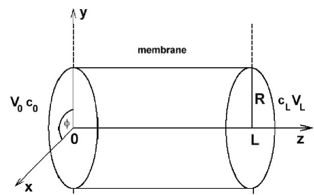
Figure 1: Channel in cartesian coordinates ($x,y,z$) with the $z$ axis along the axis of the cylinder; the cylinder has a radius $R$ and a length $L$; $V_{0},V_{L}$ are potentials and $c_{0},c_{L}$ concentrations on the left and on the right side of the channel, respectively.

The biological ion channels are ion selective Hille . The same feature is displayed in some synthetic channels Siwy ; Lev . Therefore, for simplicity, we assume that only positive ions can enter our pore. In Cole’s model Cole of electrical activity in membranes the driving force for the ions is given by the difference between the membrane potential $U=V_{in}(0)-V_{out}(L)$ and the reversal potential, which is the potential at which the current is zero. In the Goldman-Hodgkin-Katz model (GHK model) of ion flux through the channel the simplifying approximation is made that the potential gradient through the channel is constant Fall . On the other hand in experiments with synthetic membranes the driving force is caused by electrodes of potential $V_{+}$ and $V_{-}$, located in the electrolyte at macroscopic distances from the membrane (Fig. 1 in Ful1 ). Thus in both cases we put the related potential in the form:

$$\phi_{ext}(z)=V_{+}-Uz/L,$$ (1)

where $U=V_{+}-V_{-}$ and $L$ is a length of the channel. (In general, ions moving through the channel affect the local electric field. Thus, the related electric potential may be given by a more complicated function. However, if the channel is short or the ionic concentrations on either side of the membrane are small this approximation seems to be correct Sneyd .)

We consider charged channel with a given shape of internal potential $\phi^{r=0}_{int}(z)$ along the $z$ axis. Therefore, the total electric field $\vec{E}$ acting on ions inside the channel is a linear superposition of the external $\vec{E}_{ext}$ and the internal $\vec{E}_{int}$ fields, the latter one induced by charges on the wall of the channel. The goal of the following analysis is to demonstrate that the field asymmetry is sufficient to observe diode-like shape of $I-V$ relation. Let us consider two shapes of the internal potential $\phi^{r=0}_{int}(z)$ described below and presented in Fig.2. They roughly correspond to two types of channels, short biological (Fig. 2a) and long synthetic ones (Fig. 2b).

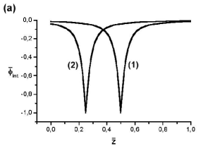
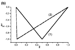
Figure 2: The shape of potential well $\overline{\phi}_{int}$ (we use dimensionless coordinate $\overline{z}=z/L$ and potential $\overline{\phi}_{int}=\beta e\phi_{int}$ a) for $\epsilon_{out}=2\epsilon_{0}$, $\epsilon_{int}=80\epsilon_{0}$, $\sigma_{g}=0,015$ e/nm², $\overline{R}=0.004$ and $\overline{g}=0.5$ ((1)-line) and $\overline{g}=0.25$ ((2)-line); b) for ratchet-like shape with $\overline{\phi}(\overline{L}_{1}=0)=\overline{\phi}(\overline{L}_{2}=1)=0$, $\overline{\phi}(\overline{g})=-1$ and $\overline{g}=0.5$ ((1)-line) and $\overline{g}=0.008$ ((2)-line).

The first potential shape we propose to consider is the potential $\phi_{int}$ of the form shown in Fig. 2a. This shape of the potential well, which results from charged residues localized at $z=g$, might simulate the situation in short biological [e.g. porin ] and synthetic Schattat channels. To find this shape we use the Eq. 12 (see Appendix) and we put the surface charge density into the formula (14) to be $\sigma(z)=\sigma_{g}\delta(z-g)$. The value of the parameter $g$ gives us the asymmetry of the function $\phi_{int}$.

The second shape, which corresponds to continuous charge distribution, is the electrostatic potential $\phi_{int}$ in the “ratchet-like” shape (Fig. 2b). This case seems to be more adequate to the long synthetic tubes in which the ratio of length to width goes to 0, thus the approximation of an infinitely long cylinder works well Ful1 .

$$\phi^{r=0}_{int}(z)=\left\{\begin{array}[]{ccc}\vspace{10pt}\phi(g)\Delta\phi^{\prime}(z-L_{1})&~{}~{}\Delta\phi^{\prime}=\displaystyle\frac{1-\phi(L_{1})/\phi(g)}{g-L_{1}},&~{}\rm{for}~{}~{}z\in[L_{1},g]\\ \vspace{10pt}\phi(g)\Delta\phi^{\prime\prime}(z-L_{2})&~{}~{}\Delta\phi^{\prime\prime}=\displaystyle\frac{1-\phi(L_{2})/\phi(g)}{g-L_{2}},&~{}\rm{for}~{}~{}z\in(g,L_{2}]\\ 0&&\rm{elsewhere}\end{array}\right.$$ (2)

where $g$ is the asymmetry parameter of this function, $\phi(g)$ is the value of the potential for $z=g$. The asymmetry of the potential is controlled by the value of the parameter $g$ (for $g=(L_{1}+L_{2})/2$ and $L_{1}=L-L_{2}$ we have the symmetric function, the most asymmetric case we have if $g\to L_{1}$ (or $g\to L_{2}$)).

III Results

The kinetic Smoluchowski equation is commonly used in various physical, chemical, etc., problems Ful . The equation describes diffusion in any physical field. Therefore a model based on this equation can be placed between these two GHK and PNP models (the GHK equation is the 1D Smoluchowski equation in a constant field).

Let us start from the 1D Smoluchowski equation that contain the electrostatic field:

$$\begin{array}[]{c}\vspace{10pt}\displaystyle\frac{\partial}{\partial t}p(z,t)=-\frac{\partial}{\partial z}j(z,t),\\ \displaystyle j(z,t)=-D\frac{\partial}{\partial z}p(z,t)+\mu E_{z}p(z,t)\end{array}$$ (3)

where $E_{z}=-\displaystyle\frac{\partial}{\partial z}\phi(z)$ is the $z$-component of electric field, $j(z,t)$ denotes probability density current, which describes the flux produced by diffusion of cations. They are driven by the difference in their probabilities of entering the pore from the left $p(0)$ and from the right $p(L)$, respectively and by ionic migration caused by difference in electric potential. We assume here that the mobility of a particle $u$ fulfills the Nernst-Einstein equation, the diffusion coefficient $D=u/\beta$, where $\beta=1/k_{B}T$. The ion mobility $\mu=ez_{c}u$, where $e$ is the electric charge, and $z_{c}$ is the cation valence.

We can write the Eq. 3 in more convenient form:

$$\frac{\partial p(z,t)}{\partial t}=\frac{\partial}{\partial z}D\displaystyle e^{-z_{c}\beta e\phi(z)}\frac{\partial}{\partial z}e^{z_{c}\beta e\phi(z)}p(z,t)=-\frac{\partial}{\partial z}j(z,t).$$ (4)

The measurable quantity is the stationary mass current $J_{i}$ ($J_{i}\neq J_{i}(t)$) flowing through the channel cross-section $\mathcal{A}=\pi R^{2}$:

$$J_{i}=\pi R^{2}j(z)$$ (5)

(we use here the identification mentioned in the introduction i.e. one ion passes the channel at the tens of nanosecond and after $10^{8}$ passages we get the measurable electric current).

For simplicity we use dimensionless coordinate $\overline{z}=z/L$, and potential $\overline{\phi}=\beta e\phi$. For the potassium cations $z_{c}=1$. Thus, the electric current resulting from mass current is:

$$I=FJ=F\displaystyle\pi R^{2}\frac{D}{L}\displaystyle\frac{c_{0}e^{\overline{\phi}_{int}(0)}-c_{1}e^{\overline{\phi}_{int}(1)-\overline{U}}}{\displaystyle\int^{1}_{0}d\overline{z}e^{\overline{\phi}_{int}(\overline{z})-\overline{U}\overline{z}}},$$ (6)

where $F$ is the Faraday’s constant. If we put $\overline{\phi}_{int}=0$ we obtain the famous Goldman-Hodgkin-Katz (GHK) current equation.

In the case of ratchet-like shape of potential $\overline{\phi}_{int}$ Eq. 2 with $\overline{L}_{1}=0$ and $\overline{L}_{2}=1$ we get the analytic solution:

$$\begin{array}[]{c}\vspace{10pt}I=FJ=\\ F\displaystyle\pi R^{2}\frac{D}{L}(c_{0}e^{\overline{\phi}(0)}-c_{1}e^{\overline{\phi}(1)-\overline{U}})/\bigg{(}\displaystyle\frac{1-e^{\overline{\phi}(\overline{g})-\overline{\phi}(0)-\overline{U}\overline{g}}}{\overline{U}-\overline{\phi}(\overline{g})\Delta\overline{\phi}^{\prime}}+\frac{e^{\overline{\phi}(\overline{g})-\overline{\phi}(1)-\overline{U}\overline{g}}-e^{-\overline{U}}}{\overline{U}-\overline{\phi}(\overline{g})\Delta\overline{\phi}^{\prime\prime}}\bigg{)}.\end{array}$$ (7)

Now, we analyze $I-V$ relations for two kinds of potential function $\overline{\phi}_{int}(z)$ that are described in Sec. Model. Let us start from the second case being ratchet-like function of $\overline{z}$. We use the analytic solution for current that is given by Eq. 7 where we put $\overline{\phi}_{int}(\overline{L}_{1}=0)=\overline{\phi}_{int}(\overline{L}_{2}=1)=0$, $\overline{R}=R/L=0.0004$, and $D_{K^{+}}=2*10^{-9}$ m²/s. The ion current through the nanochannel with no gradient of concentration ($c_{0}=c_{1}=0.01$ M) depends on both the depth of the potential well and on the degree of asymmetry of internal potential $\phi_{int}$ (see Figures 3). For the fixed depth of potential well $\overline{\phi}(\overline{g})=-9$ and different values of $\overline{g}$ (from 0.5 to 0.00001) we get various degrees of rectification. It can be clearly seen that with increasing asymmetry ($\overline{g}\to 0$) the $I-V$ characteristic tends to a diode-like shape (Fig. 3a). However the depth of potential well $\overline{\phi}(\overline{g})$ is important as well. For the lower value of $\overline{\phi}(\overline{g})=-1$ (Fig. 3b) we observe non-linear shape of $I-V$ curve for both $\overline{g}=0.5$ and $\overline{g}=0.00001$. For the asymmetric potential well the $I-V$ characteristic shows asymmetry. On the other hand, for the higher value of $\overline{\phi}(\overline{g})=-9$ (Fig. 3c) the difference between symmetric and asymmetric case is much stronger. In Fig. 3c the $I-V$ curve clearly shows the rectification (diode-like shape). The direction of the rectification depends on the value of $\overline{g}$ i.e. if it changes from 0.5 to 0.00001 or from 0.5 to 0.99999.

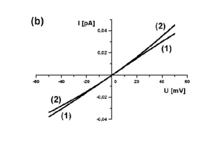
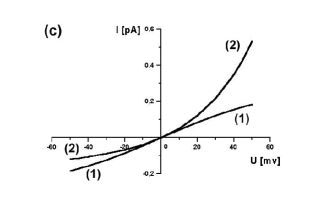
Figure 3: $I-V$ dependence for the $\overline{\phi}_{int}$ being ratchet-like function of $\overline{z}$, for $\overline{\phi}_{int}(\overline{L}_{1}=0)=\overline{\phi}_{int}(\overline{L}_{2}=1)=0$, $\overline{R}=R/L=0.0004$, $c_{0}=c_{1}=0.01$ M, $D_{K^{+}}=2*10^{-9}$ m²/s; a) $\overline{\phi}(\overline{g})=-9$ and $\overline{g}=0.5$ - solid line, $\overline{g}=0.3$ - dashed line, $\overline{g}=0.15$ - dotted line, $\overline{g}=0.00001$ - dot-dashed line; and b) $\overline{\phi}(\overline{g})=-1$, c) $\overline{\phi}(\overline{g})=-9$; in both cases for $\overline{g}=0.5$ - symmetric shape of potential function ((1)-line) and for $\overline{g}=0.00001$ - the asymmetric shape ((2)-line).

For the potential $\overline{\phi}_{int}$ showed in Fig. 2a (where $\overline{R}=R/L=0.004$), the values of boundary condition $\overline{\phi}(0)$ and $\overline{\phi}(1)$ differ from 0. What is more in the asymmetric case ((2)-line in Fig.4) the difference between them grows with increasing value of the potential well depth $\overline{\phi}(\overline{g})$ i.e. for $\overline{\phi}(\overline{g})=-10$, $\overline{\phi}(0)=-0.608$ and $\overline{\phi}(1)=-0.203$ whereas for $\overline{\phi}(\overline{g})=-40$, $\overline{\phi}(0)=-2.430$ and $\overline{\phi}(1)=-0.811$. For $c_{0}=c_{1}$ and symmetric potential function $\overline{\phi}_{int}$ the $I-V$ dependence is symmetric and weakly non-linear in both cases of $\overline{\phi}(\overline{g})$ ((1)-line in Fig. 4). For the asymmetric potential $\overline{\phi}_{int}$, we observe a weak non-linearity and the appearance of the reversal potential for the channel (Fig. 4a) which for increasing value of $\overline{\phi}(\overline{g})$ grows up (Fig. 4b). Therefore in that case we do not obtain the diode-like shape for the $I-V$ curve. Note that these results reproduce the data reported in Kos1 .

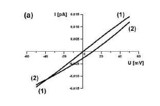
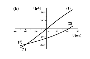
Figure 4: $I-V$ curve for the $\overline{\phi}_{int}$ being localized function of $\overline{z}$, for $\overline{R}=R/L=0.004$, $c_{0}=c_{1}=c=0.01$ M, $D_{K^{+}}=2*10^{-9}$ m²/s, the depth of potential well and the boundary conditions: a) $\overline{\phi}(\overline{g})=-10$, $\overline{\phi}(0)=\overline{\phi}(1)=-0.302$ for (1)-line, $\overline{\phi}(0)=-0.608$, $\overline{\phi}(1)=-0.203$ for (2)-line; b) $\overline{\phi}(\overline{g})=-40$, $\overline{\phi}(0)=\overline{\phi}(1)=-1.208$ for (1)-line, $\overline{\phi}(0)=-2.430$, $\overline{\phi}(1)=-0.811$ for (2)-line; in both cases for $\overline{g}=0.5$ - symmetric shape of potential function ((1)-line) and for $\overline{g}=0.25$ - the asymmetric shape ((2)-line).

In described-above cases we put $c_{0}=c_{1}$. However the boundary condition $\overline{\phi}(0)\neq\overline{\phi}(1)$ simulates the gradient of concentration $c_{0}\neq c_{1}$ in Eq. 6. Thus putting $c_{1}/c_{0}=e^{\overline{\phi}(0)}/e^{\overline{\phi}(1)}$ recovers the diode-like shape (Fig. 5).

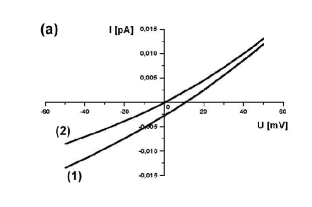
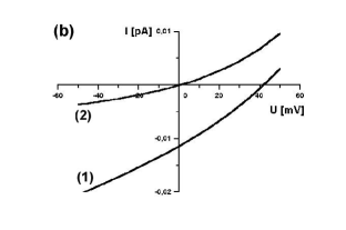
Figure 5: $I-V$ curve for the $\overline{\phi}_{int}$ being localized function of $\overline{z}$, $\overline{g}=0.25$ - the asymmetric shape of potential function, $\overline{R}=R/L=0.004$, $c_{0}=0.01$ M, $D_{K^{+}}=2*10^{-9}$ m²/s, (1)-line for $c_{1}=c_{0}$, (2)-line for $c_{1}=c_{0}e^{\overline{\phi}(0)}/e^{\overline{\phi}(1)}$, the depth of potential well and boundary condition: a) $\overline{\phi}(\overline{g})=-10$, $\overline{\phi}(0)=-0.608$, $\overline{\phi}(1)=-0.203$; b) $\overline{\phi}(\overline{g})=-40$, $\overline{\phi}(0)=-2.430$, $\overline{\phi}(1)=-0.811$.

One can obtain similar results of $I-V$ dependence for several other shapes of $\phi_{int}$ with cases of boundary conditions discussed-above.

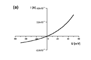
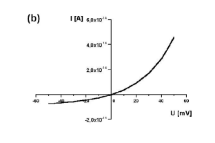
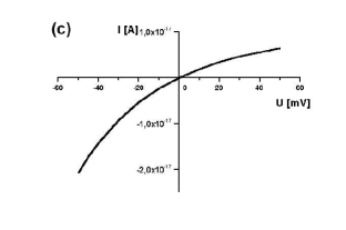
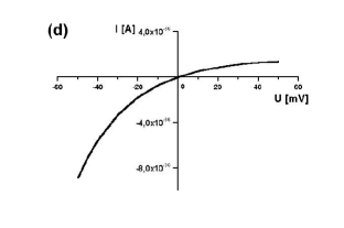
Figure 6: $I-V$ dependence for the $\overline{\phi}_{int}$ being ratchet-like function of $\overline{z}$, for $\overline{\phi}_{int}(\overline{L}_{1}=0)=\overline{\phi}_{int}(\overline{L}_{2}=1)=0$, $\overline{R}=R/L=0.0004$, $c_{0}=c_{1}=0.01$ M, $D_{K^{+}}=2*10^{-9}$ m²/s and $\overline{g}=0.00001$; a) $\overline{\phi}(\overline{g})=-5$; b) $\overline{\phi}(\overline{g})=-50$; c) $\overline{\phi}(\overline{g})=5$; d) $\overline{\phi}(\overline{g})=50$.

Finally, let us analyze the difference between the potential well and the potential barrier inside the channel. The cation that passes the negatively charged channel experiences potential well, in the contrast the anion goes over the potential barrier. We can see that the direction of the rectification is different in these two cases (Fig. 6). What is more important, the current increases with the growth of the depth of the potential well, whereas the growth of the height of the potential barrier results in dramatic decrease of the current (Fig. 6). The main point is that these two cases (potential well and barrier) are not fully symmetric. The contrast between these two cases leads us to the conclusion that the same electric field could cause enhancement of the cation current and inhibition of the anion current therefore the resulting cation selectivity of the channel. However, it has been shown recently that the selectivity of ionic channels may originate from physical mechanisms different from the electrostatics interactions, too Laio .

IV Comments and Conclusions

We found that the asymmetry of the internal potential $\phi_{int}$ coupled with the potential well depth are sufficient for the rectification observed as a diode-like shape of $I-V$ characteristic. The concentration gradient is not required for that effect. However, in the absence of internal potential $\phi_{int}(z)$), the Goldman-Hodgkin-Katz current equation, Eq. 6, gives ohmic curve $I-V$ if $\Delta c=0$ and non-ohmic shape if $\Delta c\neq 0$ Fall . In the latter case the deviation from ohmic behavior results from the gradient of concentration on both sides of the channel and is weakly non-linear. In our model, when we put $\Delta c=0$, the internal potential $\overline{\phi}_{int}$ (with the boundary values $\overline{\phi}_{int}(0)=\overline{\phi}_{int}(1)=0$) is the source of asymmetry, and gives strong non-linearity of $I-V$. Note that by varying these two factors the degree of the rectification can be intensified or diminished.

The conclusions are supported by the fact that we solve the Laplace’s equation instead of the nonlinear Poisson-Boltzmann equation (see Appendix). It allows us to avoid a misleading intuition that a nonlinear diode-like shape of $I-V$ characteristics is caused by the non-linearity of Poisson-Boltzmann equation. Apart from that, in general, it is not possible to obtain an exact solution to the Nernst-Planck (NP) equation, coupled to the electric field by means of the Poisson-Boltzmann equation. The purpose of this paper is to show that a simplified continuous model that makes use only of the electrical properties of the open channel may support our intuitive knowledge of examined phenomenon.

Moreover, our understanding of the mechanisms which account for experimental observations will enable us to design both artificial biological and synthetic channels with desired properties. Engineered nanopores may have significant applications. The properties of channels and pores that might be engineered include conductance, ion selectivity, gating and rectification, and inhibition by blockers Bayley . This prospective additionally confirms a need for the theoretical models of nanopores.

*

Appendix A

The cylinder has a radius $R$ and a height $L$, the top and bottom surfaces being at $z=L$ and $z=0$. The surface charge density on the side of the cylinder is $\sigma$ and we assume that is symmetric about the axis of the cylinder, $\sigma=\sigma(z)$. We want to find potential at any point inside the cylinder.

Figure 7: Channel in cartesian coordinates ($x,y,z$) with the $z$ axis lying along the axis of the cylinder; the cylinder has a radius $R$ and a length $L$; $\epsilon_{out}$, $\epsilon_{int}$ are dielectric constants outside and inside the channel, respectively.

There is no loss of generality if we take the infinitely long cylinder charged to prescribed charge density $\sigma$, which can differ from 0 only for $z\in[0,L]$ (Fig. 7). In cylindrical coordinates $(r,\theta,z)$ the Laplace’s equation takes form

$$\left[\frac{\partial^{2}}{\partial r^{2}}+\frac{1}{r}\frac{\partial}{\partial r}+\frac{1}{r^{2}}\frac{\partial^{2}}{\partial\theta^{2}}+\frac{\partial}{\partial z^{2}}\right]\phi=0.$$ (8)

The separation of variables is accomplished by the substitution $\phi(r,z)=P(r)Z(z)$. This leads to the two ordinary differential equations:

$$\begin{array}[]{c}\vspace{10pt}\displaystyle\frac{\partial^{2}P}{\partial r^{2}}+\frac{1}{r}\frac{\partial P}{\partial r}-k^{2}P=0\\ \displaystyle\frac{\partial Z}{\partial z^{2}}+k^{2}Z=0.\end{array}$$ (9)

We denote by $\phi_{int}$ the potential inside the channel and by $\phi_{out}$ the potential outside the channel:

$$\begin{array}[]{c}\vspace{5pt}\phi_{int}(r,z)=\int_{-\infty}^{+\infty}dk[A(k)e^{ikz}+B(k)e^{-ikz}]I_{0}(|k|r)\\ \phi_{out}(r,z)=\int_{-\infty}^{+\infty}dk[C(k)e^{ikz}+D(k)e^{-ikz}]K_{0}(|k|r).\end{array}$$ (10)

Further, these functions must satisfy the boundary conditions

$$\begin{array}[]{c}\vspace{10pt}\phi_{int}(r,z)=\phi_{out}(r,z)~{}~{}~{}~{}~{}\rm{on}~{}~{}r=R\\ \displaystyle\epsilon_{out}\frac{\partial\phi_{out}(r,z)}{\partial r}-\epsilon_{int}\frac{\partial\phi_{int}(r,z)}{\partial r}=-\sigma(z)~{}~{}~{}~{}~{}\rm{on}~{}~{}r=R,\end{array}$$ (11)

where $\epsilon_{out},~{}\epsilon_{int}$ are the dielectric constants outside and inside the channel, respectively.

The result on the $z$ axis is

$$\phi^{r=0}_{int}(z)=-\frac{1}{\sqrt{2\pi}}\int_{-\infty}^{+\infty}dke^{ikz}\hat{\sigma}(k)\mathcal{W}(|k|),$$ (12)

where

$$\mathcal{W}(|k|)=\frac{K_{0}(|k|R)}{|k|[\epsilon_{int}I_{1}(|k|R)K_{0}(|k|R)+\epsilon_{out}I_{0}(|k|R)K_{1}(|k|R)]}$$ (13)

and

$$\hat{\sigma}(k)=\frac{1}{\sqrt{2\pi}}\int_{-\infty}^{+\infty}dz\sigma(z)e^{-ikz}.$$ (14)

References

- (1) P.Yu. Apel, Yu.E. Korchev, Z. Siwy, R. Spohr, M. Yoshida, Nucl. Instrum. Meth. B 184, 337 (2001).
- (2) Z. Siwy, Y. Gu, H. Spohr, D. Baur, A. Wolf-Reber, R. Spohr, P. Apel, Y.E. Korchev, Europhys. Lett. 60, 349 (2002).
- (3) B.J. Zwolinski and H.Eyring and C. E. Reese, J. Phys. Colloid Chem., 53, 1426-1453 (1949).
- (4) P. L uger, Biochim. Biophys. Acta., 311, 423-441 (1972).
- (5) J. W. Woodbury, Eyring-rate theory model of the current-voltage relationships of ion channels in excitable membranes, in Chemical Dynamics: Papers in Honor of Henry Eyring, edited by J. O. Hirschfelder (Wiley, New York, 1971)
- (6) J. Keener, J. Sneyd Mathematical Physiology (Springer, Sunderland, MA, 1992), 2nd ed.
- (7) W. Nonner, D. P. Chen, and B. Eisenberg, J. Gen. Physiol. 113, 773-782 (1999).
- (8) B.Corry, S.Kuyucak, and S.-H. Chung, Biophys. J., 78, 2364 (2000).
- (9) B.Corry and S.Kuyucak and S.-H. Chung, J. Gen. Physiol., 114, 597-599 (1999).
- (10) D. G. Lewitt, J. Gen. Physiol. 113, 789 (1999).
- (11) A. Laio and V. Torre, Biophys. J., 76, 129-148 (1999).
- (12) Z. Siwy, P. Apel, D. Baur, D. D. Dobrev, Y. E. Korchev, R. Neumann, R. Spohr, C. Trautmann, K. Voss, Surface Science 532-535, 1061 (2003).
- (13) Z. Siwy, A. Fuliński, Phys. Rev. Lett. 89, 158101 (2002).
- (14) P.K. Kienker, W.F. DeGrado, and J.D. Lear, Proc. Natl. Acad. Sci. USA 91, 4859 (1994).
- (15) T. Okazaki, M. Sakoh, Y. Nagaoka, and K. Asami, Biophys. J. 85, 267 (2003).
- (16) E.Gorczyńska, P.L. Huddie, B.A. Miller, I.R. Mellor, R.L. Ramsey, and P.N.R. Usherwood, Pflügers Arch. Ges. Physiol. Menschen Tiere, 432, 597 (1996).
- (17) Z. Siwy, D.D. Dobrev, R. Neumann, C. Trautmann, K. Voss, Applied Physics A 76, 781 (2003).
- (18) A. Fuliński, I. D. Kosińska, and Z. Siwy, Europhys. Lett. 67, 683 (2004).
- (19) Z. Siwy, A. Fuliński, Phys. Rev. Lett. 89, 198103 (2002).
- (20) Z. Siwy, I.D. Kosińska, A. Fuliński, and C.R.Martin, Phys. Rev. Lett. 94, 048102 (2005).
- (21) I.D. Kosińska, A. Fuliński, Phys. Rev. E 72, 011201 (2005).
- (22) P. Hänggi and R. Bartussek, Brownian rectifiers: How to convert Brownian motion into directed transport, in Nonlinear Physics of Complex Systems, edited by J. Parisi, S. C. Müller, and W. Zimmermann (Springer, Berlin, 1997), Vol. 476, pp. 294-308; R. Bartussek, P. Hänggi, and J.G. Kissner, Europhys. Lett. 29, 459 (1994).
- (23) C. Marquet, A. Buguin, L. Talini, and P. Silberzan, Phys. Rev. Lett. 88, 168301 (2002).
- (24) K.K. Mon, J.K. Percus, J.Chem. Phys. 122, 214503 (2005).
- (25) A. Fuliński, Acta Phys. Pol. 29, 1523 (1998).
- (26) M. Smoluchowski, Ann. Physik 48, 1103 (1915); Phys. Z. 17, 557, 585 (1916).
- (27) M. Smoluchowski, Phys. Z., 17, 557-585 (1916).
- (28) S. Kuyucak, O. S. Andersen, and S-H. Chung, Rep. Prog. Phys. 64, 1427 (2001).
- (29) D. Appel, Nature 419, 1300 (1991); E. Toimil-Molares et al., Adv. Mater. 13, 62 (2001); E. Toimil-Molares et al., Nucl. Instr. and Meth. B 185, 192 (2001).
- (30) A. Fuliński, I. Kosińska, and Z. Siwy, New J. Phys. 7, 132 (2005).
- (31) B. Schattat, W. Bolse, S. Klaumunzer, I. Zizak, R. Scholz, Appl. Phys. Lett. 87, 173110 (2005).
- (32) T.B. Woolf and B. Roux, Proteins Struct. Funct. Genet. 24, 92 (1996).
- (33) J. Song, C.A.S.A. Minetti, M.S. Blake and M. Colombini, Biophys. J. 76, 804 (1999).
- (34) B. Hille, Ionic Channels of Excitable Membranes (Sinauer, Sunderland, MA, 1992), 2nd ed.
- (35) A.A. Lev, Y.E. Korchev, T.K. Rostovtseva, C.L. Bashford, D.T. Edmonds, and C.A. Pasternak, Proc. R. Soc. Lond. B 252, 187 (1993).
- (36) K. Cole, A Quantitative Description of Membrane Current and Its Application to Conductance and Excitation in Nerve. (University of California Press, Berkeley 1968).
- (37) Ch.P. Fall, E.S. Marland, J.M. Wagner, J.J. Tyson, Computational Cell Biology (Springer-Verlag New York, Inc. 2002).
- (38) H. Bayley and L. Jayasinghe, Mol. Membrane Biol., 21, 209-220 (2004).