Magnetic friction due to vortex fluctuation

Abstract

We use Monte Carlo and molecular dynamics simulation to study a magnetic tip-sample interaction. Our interest is to understand the mechanism of heat dissipation when the forces involved in the system are magnetic in essence. We consider a magnetic crystalline substrate composed of several layers interacting magnetically with a tip. The set is put thermally in equilibrium at temperature $T$ by using a numerical Monte Carlo technique. By using that configuration we study its dynamical evolution by integrating numerically the equations of motion. Our results suggests that the heat dissipation in this system is closed related to the appearing of vortices in the sample.

I Introduction

The friction between two sliding surfaces is one of the oldest phenomena studied in natural sciences fundamentals . In a macroscopic scale it is known that the force of friction between surfaces satisfies some rules: 1 - The friction is independent of the contacting area between surfaces. 2 - It is proportional to the normal force applied and 3 - The force of kinetic friction is independent of relative speed between surfaces. That behavior being the result of many microscopic interactions between atoms and molecules of both surfaces, it is also dependent on the roughness, temperature and energy dissipation mechanisms. Therefore, to understand friction it is necessary to understand its microscopic mechanismsNanoscience .

For several applications of now a days technology the understanding of how heat is dissipated when mobile parts are involved, plays an important role. The availability of refined experimental techniques makes it now possible to investigate the fundamental processes that contribute to the sliding friction on an atomic scale. Issues like how energy dissipates on the substrate, which is the main dissipation channel (electronic or phononic) and how the phononic sliding friction coefficient depends on the corrugation amplitude were addressed , and partially solved, by some groups. smith ; liebsch . Less known is the effect on friction of a magnetic tip moving relative to a magnetic surface. Applications of sub-micron magnets in spintronics, quantum computing, and data storage demand a huge understanding of the sub-micron behavior of magnetic materials. The construction of magnetic devices has to deal with distances of nanometers between the reading head and the storage device. That makes the study of tribological phenomena crucial to understand and produce technologically competitive devices BoLiu ; Suh ; Bhushan . In particular the dissipation of heat in magnetic dispositives is a very serious problem. For example, in a magnetic hard disk for data storage the reading head passing close to the surface of the disk transfers momentum to it. That momentum transference rises locally the temperature. Depending on the rate transfer and the capability of the disk to transfer that energy to the neighborhood some, or all, the information stored in the disk can be lost. In the last decade, the progress in the magnetic recording media and the reading head technology has made the recording density doubled almost every two years. The magnetic bit size used in the most advanced hard-disk-drives is as small as $0.5\times 0.05m^{2}$, while a giant magneto-resistance head is used to read the bit. This magnetic bit size can still be diminished by using materials with high magnetic anisotropy. However, the paramagnetic limit, when the anisotropy energy becomes comparable to the thermal fluctuations, is not far to be attained. That is a physical limitation to the technology for the production of magnetic recording media. In that case, the comprehension of the microscopic mechanism of heat dissipation is crucial. Since friction is an out-of-equilibrium phenomenon its study presents numerous theoretical and experimental challenges.

In magnetic films for which the exchange interaction is less than the separation between layers form quasi 2 dimensional (2d) magnetic planar structures. In general the magnetization of such films is confined to the plane due to shape anisotropy. An exception to that is the appearing of vortices in the system. A vortex being a topological excitation in which the integral of line of the field on a closed path around the excitation core precess by $2\pi$ ($-2\pi$) (See figure 1.). To the purpose of avoiding the high energetic cost of non-aligned moments, the vortices develop a three dimensional structure by turning out of the plane the magnetic moment components in the vortex core.evaristo-bvc For data storage purposes, magnetic vortices are of high interest since its study provides fundamental insight in the mesoscopic magnetic structures of the systemChoe .

In this paper we use a combined Monte Carlo-Molecular Dynamics (MC-MD) simulation to study the energy dissipation mechanism in a prototype model consisting of a reading head moving close to a magnetic disk surface. A schematic view is shown in figure 2. Our model consists of a magnetic tip (The reading head) which moves close to a magnetic surface (The disk surface.). The tip is simulated as a cubic arrangement of magnetic dipoles and the surface is represented as a monolayer of magnetic dipoles distributed in a square lattice. We suppose that the dipole interactions are shielded, so that, we do not have to consider them as long range interactions. This trick simplifies enormously the calculations putting the cpu time inside reasonable borders. The dipole can be represented by classical spin like variables ${\vec{S}}=S_{x}\hat{x}+S_{y}\hat{y}+S_{z}\hat{z}$. The total energy of this arrangement is a sum of exchange energy, anisotropy energy and the kinetic energy due to the relative movement between the tip and the surface as follows.

$$H=\sum_{i=1}^{N_{h}}\frac{\vec{p}_{(h-s)i}^{2}}{2m_{(h)i}}+U_{spin}+U_{h-s},$$ (1)

where $U_{spin}=U_{h}+U_{s}$.

$$U_{h} = -\frac{J_{h}}{2}\sum_{<i,j>}\left(S_{hi}^{x}\cdot S_{hj}^{x}+S_{hi}^{y}\cdot S_{hj}^{y}+\lambda_{h}S_{hi}^{z}\cdot S_{hj}^{z}\right)$$ (2)

$$- D_{h}\sum_{i=1}^{N_{h}}\left(S_{hi}^{z}\right)^{2}$$

$$U_{s} = -\frac{J_{s}}{2}\sum_{<i,j>}\left(S_{si}^{x}\cdot S_{sj}^{x}+S_{si}^{y}\cdot S_{sj}^{y}+\lambda_{s}S_{si}^{z}\cdot S_{sj}^{z}\right)$$ (3)

$$- D_{s}\sum_{i=1}^{N_{s}}\left(S_{si}^{z}\right)^{2}$$

and

$$U_{h-s}=-\sum_{i,j}J_{h-s}\left(\left|\vec{r}_{hi}-\vec{r}_{sj}\right|\right)(\vec{S}_{hi}\cdot\vec{S}_{sj})$$ (4)

with

$$J_{h-s}\left(\left|\vec{r}_{hi}-\vec{r}_{sj}\right|\right)=J_{0}\exp\{-\alpha\left(\vec{r}_{hi-sj}-r_{0}\right)^{2}\}$$ (5)

In equation 1 the first term, ${\vec{p}_{(h-s)i}^{2}}/{2m_{(h)i}}$ , stands for the relative kinetic energy : surface-reading head (s-h). The second term, $U_{spin}$, accounts for the magnetic dipoles interactions: in the tip ($U_{h}$) and in the surface ($U_{s}$). The last term, $U_{h-s}$, is the interaction energy between the tip and the surface. The symbol $<ij>$ means that the sums are to be performed over the first neighbors. For the tip-surface interaction, we suppose that the coupling, $J_{h-s}$, is ferromagnetic. By considering that $J_{h-s}$ is a function of distance, will allow us to study the effects of the relative tip-surface movement. The exchange anisotropic term $\lambda$, controls the kind of vortex which is more stable in the lattice.

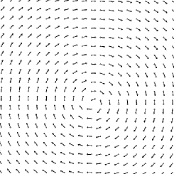
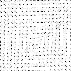
Figure 1: Schematic view of a vortex (left) and anti-vortex (right) for spins of the same length.

There is a critical value of the anisotropy, $\lambda_{c}\approx 0.7J$ evaristo-bvc , such that for $\lambda<\lambda_{c}$ the spins inside the vortex core minimizes the vortex energy by laying in an in-plane configuration. For $\lambda>\lambda_{c}$ the configuration that minimizes the vortex energy is for the spins close to the center of the vortex to develop a large out-of-plane component. The site anisotropy, $D$, controls the out-of-plane magnetization of the model. It is well known that a quasi-two dimensional system with interaction as in equation 2 undergoes a $BKT$ phase transition for $D_{h}$ sufficiently small (In general $D/J<<\lambda$.), at some critical temperature $T_{BKT}$. If, $D/J=\lambda$ = 0, $T_{BKT}\approx 0.7$. For $D/J>>\lambda$ the system has a second order phase transition at $T_{c}$ which depends on $D$.

In the sections below we will discuss the importance of vortex formation for the energy dissipation of a magnetic material. In the section II we introduce general aspects of the numerical method used, in the section III we discuss our results and in section IV we present our conclusions.

II Simulation Background

In this section we describe the numerical approach we have used to simulate the model. The simulation is done by using a combined Monte Carlo-Molecular Dynamics (MC-MD) procedure. The particles in our simulation move according Newton’s law of motion which can be obtained by using the hamiltonian 1. The spins evolve according to the equation of motion gerling

$$\frac{d\vec{S}_{hi,si}}{dt}=-\vec{S}_{hi,si}\times\frac{\partial H}{\partial\vec{S}_{hi,si}}.$$ (6)

As we are mainly interested in the magnetic effects we consider the particles as fixed letting the tip slid over the surface. This generates a set of $3N+3$ coupled equations of motion which are solved by increasing forward in time the physical state of the system in small time steps of size $\delta t=10^{-3}J^{-1}$. The resulting equations are solved by using Runge-Kutta’s method of integrationAllen ; Rapaport ; Berendsen .

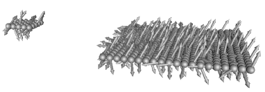
Figure 2: Schematic view of our simulation arrangement. The tip is simulated as a $5\times 5$ rigid lattice of particles each carrying a spin $\vec{S}$. The surface is simulated as an arrangement of size $20\times 20$. The tip is allowed to slid over the surface with initial velocity $v=v_{0}\hat{x}$. Periodic boundary conditions are used for the in plane directions of the surface. The arrows represent the spins directions.

The surface is arranged as a rigid $20a\times 20a$ square lattice with periodic boundary conditions in the $xy$ direction, where $a$ is the lattice spacing. The head is simulated as a rigid $5a\times 5a$ square lattice. With no loss of generality the lattice spacing will be taken as $a=1$ from now on. In figure 2 we show a schematic view of the arrangement used in our simulation. Initially we put the tip at a large distance from the surface, so that, $J_{h-s}=0$. By using the MC approach we equilibrate the system at a given temperature, $T$. By controlling the energy of the system we consider that the system is in equilibrium after $10^{5}$ MC steps. Once the thermal equilibrium is reached we observe the evolution of the separated systems for a small time interval, $\tau$, for posterior comparison. After that an initial velocity, $v=v_{0}\hat{x}$ is given to the tip. We follow the system’s evolution by storing all positions, velocities and spin components at each time step for posterior analysis. A quantity of paramount importance for us is the vortex density, $\varphi_{v}(t)$, at the surface layer. We calculate the vortex density as a function of temperature and time for several values of the parameters $\lambda_{s}$, $\lambda_{h}$ and $D_{s}$, $D_{h}$. As discussed in the following the vortex density will be related to energy dissipation. The energy is measured in units of $J_{h}=J_{s}=J$, temperature in units of $J/k_{B}$, time in units of $J^{-1}$ and velocity in units of $a/J^{-1}$ where $k_{B}$ is the Boltzmann constant.

III Results

The system is simulated for several temperatures and anisotropy parameters. In all of them we have fixed $J_{h}=J_{s}=J$, $J_{0}=2J$ and $\alpha=1$. In the first set of simulations we use $\lambda_{s}=\lambda_{h}=1J$ and the site anisotropy $D_{s}=D_{h}=0.1J$, $-0.1J$ to obtain a system with out-of-plane (Ising-like) and in-plane ($XY$) symmetries respectively. In the second set, we put $D_{s}=D_{h}=0$ and $\lambda_{s}=\lambda_{h}=0.6J,0.9J$ to get vortices with in-plane and out-of-plane cores respectively.

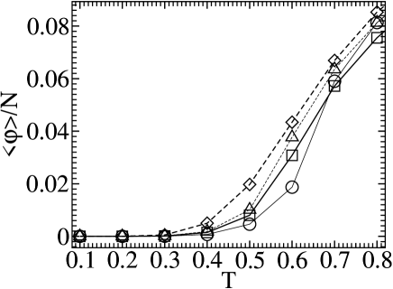
Figure 3: Vortex Density as a function of the temperature. The symbols are for $\lambda_{s}=\lambda_{h}=1$ with $D_{h}=D_{s}=0.1J$ ($\circ$), $D_{h}=D_{s}=-0.1J$ ($\square$) and $D_{s}=D_{h}=0$ with $\lambda_{s}=\lambda_{s}=0.6J$ ($\Diamond$) and $\lambda_{h}=\lambda_{s}=0.9J$ ($\vartriangle$). The lines are only guides to the eyes.

Before we start the time evolution, we have to know how the vortex density, $\varphi_{v}$, depends on the temperature. In figure 3 we show a plot of $\varphi_{v}$ as a function of the temperature for the simulated models. The vortex density increases monotonically with $T$. If there is any relation between vortices and energy dissipation, it is natural to think that an increase in the vortex density is related to an increase in temperature.

With the head far from the surface, we start the time evolution of the system at $t=0$ with $v=0$. This part of the simulation serves as a guide to the rest of the simulation. Only thermal fluctuations of the vortex density can be seen. At $t=200$ the tip is released with initial velocity $v_{0}$. For $t>200$, the reading head starts to interact with the surface. Some kinetic energy is transferred from the head to the surface and we expect the vortex density to increase. We will see in the following that depending on the initial conditions and the symmetry of the system (See equation 1) several things can happen.

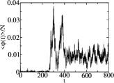
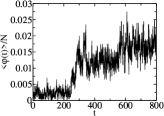
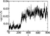
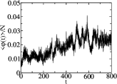
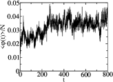
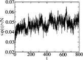
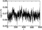
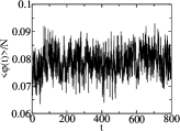
Figure 4: Vortex Density as a function of time for $D_{h}=D_{s}=0.1J$ and $\lambda_{s}=\lambda_{s}=1J$. The graphics from left to right and top to bottom correspond to the temperatures $T=0.1,0.2,0.3,0.4,0.5,0.6$. The system has an out-of-plane symmetry.

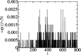
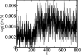
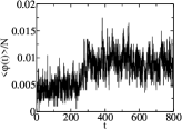
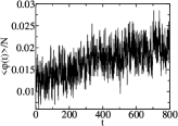
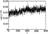
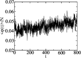
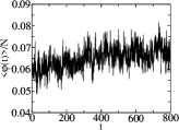
Figure 5: Vortex Density as a function of time for $D_{h}=D_{s}=-0.1J$ and $\lambda_{s}=\lambda_{s}=1J$. Temperatures are the same as in figure 4. The system has an in-plane symmetry.

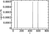
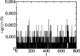
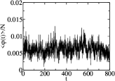
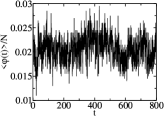
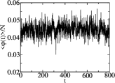
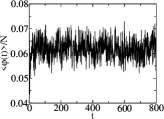
Figure 6: Vortex Density as a function of time for $\lambda_{s}=\lambda_{s}=0.6J$ and $D_{h}=D_{s}=0$. Temperatures are the same as in figure 4. The vortex has an in-plane structure.

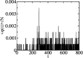
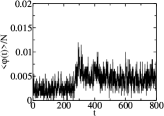
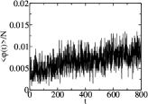
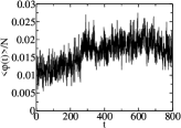
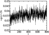
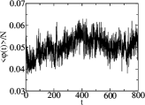
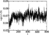
Figure 7: Vortex Density as a function of time for $\lambda_{s}=\lambda_{s}=0.9J$ and $D_{h}=D_{s}=0$. Temperatures are the same as in figure 4. The vortex has an out-of-plane structure.

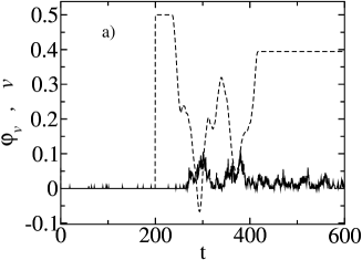
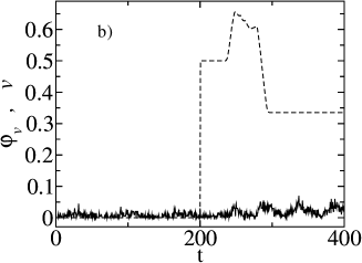
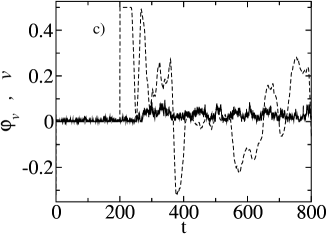
Figure 8: Instantaneous velocity and vortex density as a function of time for $D_{h}=D_{s}=0.1J$ and $\lambda_{s}=\lambda_{s}=1J$. The full line is the vortex density and the dashed line is for the instantaneous velocity. From top to bottom $T=0.1,0.2$. The initial velocity is $v=0.5$ in all cases. The vortex density is multiplied by a factor $2$ as a matter of clarity.

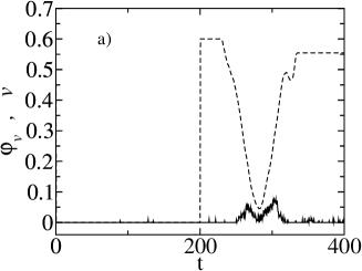
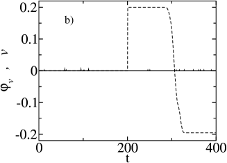
Figure 9: Instantaneous velocity and vortex density as a function of time for $D_{h}=D_{s}=0.1J$ and $\lambda_{s}=\lambda_{s}=1J$. The full line is the vortex density and the dashed line is for the instantaneous velocity. The temperature is $T=0.2$ in both cases. From top to bottom the initial velocity is $v=0.6,0.2$. The vortex density is multiplied by a factor $2$ as a matter of clarity.

In the figures 4 to 7 we show plots of the averaged vortex density as a function of the time for the set of the simulated parameters as discussed above. In each figure, the graphics from left to right and top to bottom correspond to $T=0.1,0.2,0.3,0.4,0.5,0.6,0.7$ and $0.8$.

For the system with out-of-plane symmetry (Figure 4) we observe that for low temperature the vortex density augments when the tip passes over the surface. Initially the vortex density grows reaching quickly a constant average. For higher temperature the vortex density is almost insensitive to the tip indicating that the energy transfer becomes more difficult. At low temperature it is easier to excite the vortex mode since they have low creation energy due to the out-of-plane spin component. At higher temperature the system is already saturated and creating a new excitation demands more energy. For the in-plane symmetry (Figure 5) the situation is opposite. At low temperature there is no energy transfer to vortex modes. Creating a vortex demands much energy because the spin component of the vortex is almost whole in-plane. At higher temperature the system is soft so that it can absorb energy augmenting the vortex density. Eventually it reaches saturation at high enough temperature. For the case when the vortex has an in-plane-symmetry ($\lambda<\lambda_{c}$), shown in figure 6, the average vortex density is constant even at higher temperatures. For ($\lambda>\lambda_{c}$) (Figure 7) the situation is similar to that where the system has a global out-of-plane symmetry (Compare to figure 4).

In figure 8 we show the velocity of the head and the vortex density as a function of time plotted in the same graphic for some interesting situations. The vortex density is multiplied by a factor of $2$ as a matter of clarity. In the first plot we observe that the kinetic energy of the tip is transferred to the surface. The head stops, moves back and forth and escapes from the surface influence. At higher temperatures the situation is a bit more complex. Depending on the initial condition the head passes through the surface region just augmenting the vortex density (8.b) or it can be trapped in the surface region, as seen in figure 8.c. The cost for the increase in the vortex density is a decrease in the kinetic energy.

In figure 9 $a$ and $b$ we show the velocity and vortex density as a function of time for two different initial velocities ($v=0.6,0.2$ respectively), at the same temperature $T=0.2$. For the higher velocity, the tip decreases its velocity almost up to stop, however, its kinetic energy is sufficient to go across the surface region. For a lower velocity, figure 9.$b$, the tip collides elastically with the surface. Because there is no lost in kinetic energy the vortex density is conserved. We note that the increase in the vortex density it is not an instantaneous response to the diminishing of the kinetic energy of the tip. It may be due to an intermediate mechanism: The kinetic energy is used to excite spin waves in the surface. Because there is no mechanism of energy dissipation, part of the energy contained in the spin waves is transferred to vortex excitations.

IV Conclusions

We have used Monte Carlo and spin dynamics simulation to study the interaction between two magnetic mobil parts: a magnetic reading head dislocating close to a magnetic surface. Our interest was to understand the mechanism of heat dissipation when the forces involved in the system are magnetic in essence. To simulate the surface we have considered a magnetic crystalline substrate interacting magnetically with a magnetic tip. From the results presented above we have strong evidences that vortices play an important role in the energy dissipation mechanism in magnetic surfaces. The augmenting of the vortex density excitations in the system increases its entropy. That phenomenon can blur any information eventually stored in magnetic structures in the surface. An interesting result is the velocity behavior of the tip passing close to the surface. In principle we should expect that the velocity will always diminish, as an effect of the interaction with the surface. However, for certain initial conditions the effect is opposite. The tip can oscillate, be trapped over the surface or even be repelled. In the case of an elastic collision the vortex density remains unchanged. If the vortex density increases the tip’s kinetic energy diminishes. However, the increase in the vortex density is not an instantaneous response to the diminishing of the kinetic energy of the tip. We suspect that an intermediate mechanism involving spin wave excitations is present intermediating the phenomenon.

The effects on friction observed in our simulations demonstrate that when pure magnetic forces are involved they are quite different from ordinary friction. There are two points that should be interesting to study: The effect of normal forces applied to the system and how the observed effects depend on the contacting area between surfaces.

V Acknowledgments

Work partially supported by CNPq (Brazilian agencies). Numerical work was done in the LINUX parallel cluster at the Laboratório de Simulação Departamento de Física - UFMG.

References

- (1) Fundamentals of friction, Macroscopic and microscopic processes, edited by I.L. Singer and H. M. Pollock (Kluwer, Dordrecht)1992.
- (2) E. Meyer, R.M. Overney, K. Dransfeld and T. Gyalog, Nanoscience - Friction and Rheology on the Nanometer Scale, (World Scientific Publishing, Singapore, 1998).
- (3) A. Liebsch, S. Gonc¸alves and M. Kiwi, Phys. Rev. B 60,(1999)5034.
- (4) E. D. Smith, M. O. Robbins and M.k Cieplak, Phys. Rev. B 54,(1996)8252.
- (5) B. E. Argyle, E. Terrenzio and J. C. Slonczewski, Phys. Rev. Lett. 53,(1984)190.
- (6) J. P. Park, P. Eames, D. M. Engebretson, J. Berezovsky and P. A. Crowell, Phys. Rev. B 67,(2003)20403.
- (7) Th. Gerrits, H. A. M. van den Berg, J. Hohlfeld, K. Bär and Th. Rasing, Nature 418, (2002)509.
- (8) Bo Liu, Jin Liu and Tow-Chong Chong, J. Mag. Mag. Mater. 287(2005) 339345
- (9) A.Y. Suh and A.A. Polycarpou, J. Applied Phys. 97,104328 (2005)
- (10) B. Bhushan, J. Magn. Magn. Mater. 155, (1996) 318-322
- (11) J.E.R. Costa and B.V. Costa, Phys. Rev. B 54, (1996)994; J.E.R. Costa, B.V. Costa and D.P. Landau, Phys. Rev. B 57, (1998)11510; B.V. Costa, J.E.R. Costa and D.P. Landau, J. Appl. Phys. 81 (1997), 5746.
- (12) S.-B Choe, Y. Acremann, A. Scholl, A. Bauer, A. Doran, J. Stöhr and H. A. Padmore, Science 304,(2004) 402.
- (13) D.P. Landau and R.W. Gerling, J. Magn. Magn. Mater. 104-107 (1992)843
- (14) M.P. Allen and D.J. Tildesley, Computer Simulation of Liquids (Oxford Scince Publications, New York, 1992)
- (15) D.C. Rapaport, The Art of Molecular Dynamic Simulation (Cambridge University Press, New York, 1997)
- (16) H. J. C. Berendsen and W. F. Gunsteren Pratical Algorithms for Dynamic Simulations. Pag. 43-65.