Group delay in Bragg grating with linear chirp

Abstract

An analytic solution for Bragg grating with linear chirp in the form of confluent hypergeometric functions is analyzed in the asymptotic limit of long grating. Simple formulas for reflection coefficient and group delay are derived. The simplification makes it possible to analyze irregularities of the curves and suggest the ways of their suppression. It is shown that the increase in chirp at fixed other parameters decreases the oscillations in the group delay, but gains the oscillations in the reflection spectrum. The conclusions are in agreement with numerical calculations.

PACS 42.81.Wg; 78.66.-w

1 INTRODUCTION

Optical filters based on fiber gratings attract particular interest because of their applications in high-speed lightware communications [1], fiber lasers [2] and sensors [3]. The Bragg reflector is based on periodic modulation of the refractive index along the line [4, 5]. Gratings that have a nonuniform period along their length are known as chirped. The theory of linearly chirped grating holds the central place in the fiber optics. Chirped grating is of importance because of its applications as a dispersion-correcting or compensating devices [6]. The study of linearly chirped grating is also helpful for approximate solution of more general problem of complex Gaussian modulation [7]. The group delay as a function of wavelength is a linear function with additional oscillations. For applications the problem is to minimize the amplitude of regular oscillations and the ripple resulting from the errors of manufacturing [8].

The purpose of this work is to present and study a solution of the equations for amplitudes of coupled waves in quasi-sinusoidal grating with quadratic phase modulation. The solution of coupled-wave equations is derived in terms of the confluent hypergeometric functions. Their asymptotic expansion in terms of Euler $\Gamma$-functions makes it possible to obtain relatively simple formulas for reflectivity and group delay. The simplification enables analysis of irregularities of the curves and suggestions on the ways of their suppression.

The paper is organized as follows. The equations for amplitudes in the grating with quasi-sinusoidal modulated refractive index are derived in Sec. 2. Their analytic solutions are obtained and compared with numerical results in Sec. 3. The asymptotic behavior is treated in Sec. 4. Some estimations and qualitative explanations are presented in Sec. 5. Possible methods to suppress the oscillations are summarized in Sec. 6.

2 Equations for slow amplitudes

Consider a single-mode fiber with the weakly modulated refractive index $n+\delta n(z)$. Steady-state electric field $E(z)$ satisfies one-dimensional Helmholtz equation

$$\frac{d^{2}E}{dz^{2}}+k^{2}\left[1+\frac{2\delta n(z)}{n}+\left(\frac{\delta n(z)}{n}\right)^{2}\right]E=0,\quad k=\frac{\omega n}{c},$$ (1)

where $z$ is the coordinate, $k$ is the wavenumber in glass outside the grating, where $\delta n(z)=0$, $\omega,c$ are the frequency and speed of light. The addition to mean refractive index may be a function with phase and amplitude modulation. A family of analytical solutions for amplitude modulation was obtained in [9]. Below we treat a case of phase modulation

$$\frac{\delta n(z)}{n}=2\beta\cos\theta(z),$$ (2)

where $\theta(z)$ is the phase, constant $\beta$ is the modulation depth. Since $\beta\ll 1$ we neglect the quadratic term in (1). The phase is general quadratic function

$$\theta(z)=\alpha z^{2}/2+\kappa z+\theta_{0},$$ (3)

where $\kappa$ is the frequency of spatial modulation at $z=0$, $\theta_{0}$ is the constant phase shift. The condition of slow phase variation is

$$\left|\frac{d\theta}{dz}-\kappa\right|\ll\kappa.$$ (4)

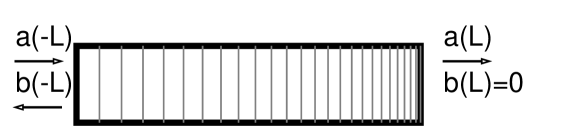
Figure 1: The statement of the scattering problem.

Let us introduce complex amplitudes $a,b$ of waves running in positive and negative directions

$$E=a\mathrm{e}^{\mathrm{i}kz}+b\mathrm{e}^{-\mathrm{i}kz}.$$

Keeping only resonant terms and neglecting the parametric resonance of higher orders at the detuning

$$q=k-\kappa/2\ll k_{0}=\kappa/2,$$ (5)

we get the equations for coupled waves

$$a^{\prime}=\mathrm{i}k_{0}\beta\mathrm{e}^{-2\mathrm{i}kz+\mathrm{i}\theta(z)}b,\quad b^{\prime}=-\mathrm{i}k_{0}\beta\mathrm{e}^{2\mathrm{i}kz-\mathrm{i}\theta(z)}a,$$ (6)

where prime denotes $z$-derivative.

Set (6) conserves $|a|^{2}-|b|^{2}$, since the signs in right-hand sides of equations are different. The same equations with identical signs conserve the sum of populations $|a|^{2}+|b|^{2}$ and describe the amplitudes of probability in two-state quantum system. The exact solutions in this case are of importance in quantum optics, then they are studied in details [10, 11]. Within the limits of resonance approximation (5) we replace $k$ in front of exponents (6) by $k_{0}$.

Finding the derivatives of (6) with respect to $z$ we get complex conjugated second-order equations

$$a^{\prime\prime}-\mathrm{i}\alpha\left(z-z_{0}\right)a^{\prime}-k_{0}^{2}\beta^{2}a=0,\quad b^{\prime\prime}+\mathrm{i}\alpha\left(z-z_{0}\right)b^{\prime}-k_{0}^{2}\beta^{2}b=0.$$ (7)

Here $z_{0}=(2k-\kappa)/\alpha=2q/\alpha$ is the coordinate of resonance point for the wave with wavenumber $k$. It is the turning point where the wave with given $q$ is reflected. The parametric resonance for central wavenumber $q=k-\kappa/2=0$ occurs at $z=0$. Let $\alpha>0$, then for the red detuning $q<0$ we have $z_{0}<0$, in opposite case $q>0$ of blue detuning $z_{0}>0$.

Consider the Bragg grating written in the interval $-L\leqslant z\leqslant L$. The problem of left reflection coefficient calculation is illustrated by Fig. 1. Boundary conditions are defined by the scattering problem statement. We set amplitude $b$ at the right end equal to zero

$$b(L)=0$$ (8)

and get the reflection and transmission coefficients

$$r=\frac{b(-L)}{a(-L)},\quad t=\frac{a(L)}{a(-L)}.$$ (9)

The chirp is weak and satisfy (4), then the equations for complex amplitudes are valid when

$$\alpha L\ll\kappa.$$ (10)

Note that set (7) is symmetric under transformation $\alpha\to-\alpha,q\to-q,a\leftrightarrow b$. Then the right reflection coefficient can be obtained from the expression for left one by changing signs of parameters $\alpha$ and $q$.

3 Solution

Equations (7) are reduced to the confluent hypergeometric form by the substitution $t=\mathrm{i}\alpha(z-z_{0})^{2}/2$:

$$t\ddot{a}+\left(\frac{1}{2}-t\right)\dot{a}+\mathrm{i}\eta a=0,$$

where dot denotes the derivative with respect to new variable $t$, $\eta=\beta^{2}k_{0}^{2}/2\alpha$ is the adiabatic parameter. The equation for second amplitude $b$ is complex conjugated. The general solutions at $-L<z<L$ are linear combinations

$$a(z)=A_{1}u_{1}(z)+A_{2}u_{2}(z),\quad b(z)=B_{1}u_{1}^{*}(z)+B_{2}u_{2}^{*}(z)$$ (11)

of the Kummer confluent hypergeometric functions [12]:

$$u_{1}=F\left(-\mathrm{i}\eta;{\scriptstyle\frac{1}{2}};\mathrm{i}\alpha(z-z_{0})^{2}/2\right),$$

$$u_{2}=(z-z_{0})F\left({\scriptstyle\frac{1}{2}}-\mathrm{i}\eta;{\scriptstyle\frac{3}{2}};\mathrm{i}\alpha(z-z_{0})^{2}/2\right);$$ (12)

$$F(a;c;x)=1+\frac{a}{c}\frac{x}{1!}+\frac{a(a+1)}{c(c+1)}\frac{x^{2}}{2!}+\dots,$$

where $A_{1},A_{2},B_{1},B_{2}$ are constants and the asterisk denotes the complex conjugation. The solution was obtained in [13] for optical waveguide. The solution for coupled-wave equations with identical signs has been obtained in the context of nonadiabatic population inversion in two-level system [14].

The relations between constants can be obtained from set (6) near resonance point $z=z_{0}$ where $a=A_{1}+A_{2}(z-z_{0})+O(z-z_{0})^{2},b=B_{1}+B_{2}(z-z_{0})+O(z-z_{0})^{2}$:

$$\frac{A_{2}}{B_{1}}=\mathrm{i}k_{0}\beta\mathrm{e}^{\mathrm{i}\theta_{0}-\mathrm{i}\alpha z_{0}^{2}/2},\quad\frac{B_{2}}{A_{1}}=-\mathrm{i}k_{0}\beta\mathrm{e}^{-\mathrm{i}\theta_{0}+\mathrm{i}\alpha z_{0}^{2}/2}.$$ (13)

The right boundary condition (8) yields the ratio of coefficients $A_{1}$ and $A_{2}$

$$\rho=\frac{A_{1}}{A_{2}}=\frac{1}{k_{0}^{2}\beta^{2}}\frac{B_{2}}{B_{1}}=-\frac{F\left(\mathrm{i}\eta;{\scriptstyle\frac{1}{2}};-\mathrm{i}\alpha(L-z_{0})^{2}/2\right)}{\beta^{2}k_{0}^{2}(L-z_{0})F\left({\scriptstyle\frac{1}{2}}+\mathrm{i}\eta;{\scriptstyle\frac{3}{2}};-\mathrm{i}\alpha(L-z_{0})^{2}/2\right)}.$$ (14)

The left reflection and transmission coefficients (9) can be expressed in terms of confluent hypergeometric functions

$$r=\frac{\mathrm{e}^{-\mathrm{i}\theta_{0}+\mathrm{i}\alpha z_{0}^{2}/2}}{\mathrm{i}k_{0}\beta}\frac{u_{1}^{*}(-L)+\beta^{2}k_{0}^{2}\rho u_{2}^{*}(-L)}{\rho u_{1}(-L)+u_{2}(-L)},\quad t=\frac{\rho u_{1}(L)+u_{2}(L)}{\rho u_{1}(-L)+u_{2}(-L)},$$ (15)

where functions $u_{1,2}$ are defined by (12) and $\rho$ is defined by (14).

Figure 2: (a) Reflection spectrum $R(q)$ at $\alpha=600~{}\mbox{cm}^{-2},L=0.5~{}\mbox{cm},k_{0}=6\times 10^{4}~{}\mbox{cm}^{-1}$, from the top down $\beta=\beta_{0},\beta_{0}/2,\beta_{0}/4$, where $\beta_{0}=0.67\times 10^{-3}$. (b) A part of the lower curve $\beta=\beta_{0}/4$, crosses denote the numerical result.

The reflection spectrum, i.e., the reflectivity $R=|r|^{2}$ as a function of detuning $q$, is shown in Fig. 2 (a). The central frequency of the spectrum comes to resonance at $z=0$, in the middle of grating. The central part has a flat top at high adiabatic parameter, as the upper curve shows, and the maximal reflectivity is close to 1. The width of central part is proportional to the length $L$. The reflectivity is relatively high if the turning point $z_{0}$ lies inside the grating $|z_{0}|<L$. This inequality gives the bandwidth $|q|<\alpha L/2$. There is no parametric resonance at higher detuning, when $|z_{0}|>L$, and the reflectivity is small. Fig. 3 (a) shows how the bandwidth grows up with the chirp parameter $\alpha$ at fixed modulation depth $\beta$. The adiabatic parameter decreases with $\alpha$, then the reflectivity in the center decreases from curve to curve.

Figure 3: (a) Reflection spectrum from the top down at $L=0.5~{}\mbox{cm},\beta=0.33\times 10^{-3},k_{0}=6\times 10^{4}~{}\mbox{cm}^{-1}$ and $\alpha=\alpha_{0},2\alpha_{0},3\alpha_{0},$, where $\alpha_{0}=600~{}\mbox{cm}^{-2}$. (b) A part of the lower curve $\alpha=3\alpha_{0}$, crosses denote the numerical result.

The spectrum was recalculated numerically by $T$-matrix approach. The initial Helmholtz equation (1) was solved numerically with neither approximation of slow envelope, nor quadratic term $(\delta n/n)^{2}$ neglecting. The number of layers per period of spatial modulation was fixed at $N=32$, then the step varied along the grating. The spectra for $n=1.5$ and the same parameters are shown in Fig. 2 (b) by crosses. The numerical results are very close to analytical, since both dimensionless parameters controlling the validity of coupled-wave approximation are small: $\beta\sim 10^{-3},\alpha L/\kappa\sim 5\times 10^{-3}$. At higher parameter $\alpha$ the deviation of coupled-wave equations solutions from that of Helmholtz equation increases, but not dramatically, as shown in Fig. 3 (b). The origin of the deviation is resonance approximation (5). We replace $k$ by $k_{0}$ in coupled-mode equations (6), while the Helmholtz wave equation (1) involves $k$. Comparing Fig. 2 (a) and Fig. 3 (b) we see that the latter involves higher detuning, then the deviation is greater at higher $q=k-k_{0}$.

Figure 4: (a) Group delay (ps) as a function of detuning $q$ (cm^-1) at $\alpha=600~{}\mbox{cm}^{-2},L=0.5~{}\mbox{cm},k_{0}=6\times 10^{4}~{}\mbox{cm}^{-1}$, from the top down $\beta=\beta_{0},\beta_{0}/2,\beta_{0}/4$, where $\beta_{0}=0.67\times 10^{-3}$. (b) Comparing with numerical calculation denoted by dots.

The group delay found from analytical solution (15) is plotted in Fig. 4 (a) at the same parameters as the reflection spectrum in Fig. 2. The deviation of curves from the linear dependence, the group delay ripple, manifests itself as oscillations with variable frequency. The frequency grows up towards the blue end of spectrum in agreement with results from [15, 5]. For the negative chirp (or when the incident light enters from the right) the frequency grows up towards the red edge of spectrum. The maximum deviation from the averaged slope decreases with decreasing modulation depth $\beta$. Meanwhile, the ripple in reflectivity increases for small $\beta$. A fragment of group delay characteristics is shown in Fig. 4 (b) along with numerical calculations. Dots obtained from numerical calculation are very close to the curve given by analytical formula.

It is difficult to analyze the solution in its general form. In particular the cumbersome expression for group delay, the derivative of (15) with respect to the detuning, is not presented here. Let us simplify expressions using the asymptotics of Kummer functions in the next section.

4 Asymptotics

The asymptotic expressions for the reflection coefficient can be obtained from (15) in two cases. The first case is the resonance condition at the left end, namely, detuning $q=-\alpha L/2$ for which $z_{0}=-L$. In this case it follows from (12) that $u_{1}(-L)=1,u_{2}(-L)=0$, and then from (15)

$$r\approx\frac{\mathrm{e}^{-\mathrm{i}\theta_{0}+\mathrm{i}\alpha L^{2}/2}}{\mathrm{i}k\beta\rho}\approx-\frac{\mathrm{e}^{-\mathrm{i}\theta_{0}+\mathrm{i}\alpha L^{2}/2}}{\sqrt{\mathrm{i}\eta}}\frac{\Gamma(1/2-\mathrm{i}\eta)}{\Gamma(-\mathrm{i}\eta)},$$ (16)

$$R=|r|^{2}\approx\tanh\pi\eta.$$ (17)

The other case is when the resonance point $z_{0}$ being far from both ends inside the grating: $|q|<\alpha L/2$ and $\alpha(z_{0}\pm L)^{2}/2\gg 1$. The asymptotic expression of the confluent hypergeometric functions [12] at $|\mathrm{arg}\,x|<\pi$

$$F(a;c;x)\approx\frac{\Gamma(c)}{\Gamma(c-a)}\left(\frac{\mathrm{e}^{\mathrm{i}\pi\epsilon}}{x}\right)^{a}+\frac{\Gamma(c)}{\Gamma(a)}\mathrm{e}^{x}x^{a-c},\quad\epsilon=\begin{cases}+1,&\textrm{Im}\,x>0,\\ -1,&\textrm{Im}\,x<0\end{cases}$$ (18)

allows one to simplify expression (15).

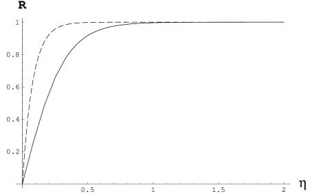
Figure 5: The reflectivity $R$ as a function of adiabatic parameter $\eta$ at $z_{0}=-L$ (solid line) and at $z_{0}=0$ (dashed).

The reflection coefficient can be written using (12)

$$r\approx-\sqrt{R_{0}}\mathrm{e}^{\mathrm{i}\phi-\mathrm{i}\pi/4+2\mathrm{i}q^{2}/\alpha-\mathrm{i}\theta_{0}}\left[\frac{\alpha}{2}\left(L+\frac{2q}{\alpha}\right)^{2}\right]^{-2\mathrm{i}\eta}\times$$

$$\frac{1+\mathrm{e}^{+\mathrm{i}\pi/4-\mathrm{i}\phi}\sqrt{\frac{\eta}{R_{0}}}\left(\psi_{+}^{2\mathrm{i}\eta-1/2}\mathrm{e}^{-\mathrm{i}\psi_{+}}+\psi_{-}^{2\mathrm{i}\eta-1/2}\mathrm{e}^{-\mathrm{i}\psi_{-}}\right)}{1+\sqrt{\eta R_{0}}\left(\psi_{+}^{-2\mathrm{i}\eta-1/2}\mathrm{e}^{\mathrm{i}\psi_{+}+\mathrm{i}\phi-\mathrm{i}\pi/4}+\psi_{-}^{2\mathrm{i}\eta-1/2}\mathrm{e}^{-\mathrm{i}\psi_{-}-\mathrm{i}\phi+\mathrm{i}\pi/4}\right)},$$ (19)

where $\psi_{\pm}(q)=\alpha(L\pm 2q/\alpha)^{2}/2$, $\phi=\mbox{arg}[\Gamma(\mathrm{i}\eta)\Gamma(1/2+\mathrm{i}\eta)]$, $R_{0}=1-\mathrm{e}^{-4\pi\eta}$ and we omit terms of the order of $1/\alpha L^{2}\ll 1$. The enumerator and denominator of the fraction in the second line of (19) are close to 1, if $\psi_{\pm}\gg 1$. Then the formula for reflectivity becomes simple

$$R\approx R_{0}=1-\mathrm{e}^{-4\pi\eta}.$$ (20)

Both curves (17) and (20) are shown in Fig. 5. One can see their saturation, moreover, when the turning point $z_{0}=-L$, the saturation occurs later than when the turning point is far from both ends.

The group delay obtained from (19) is

$$f=\frac{d\mathrm{Arg}\,r}{d\omega}=\frac{n}{c}\frac{d\textrm{Im}\,\ln r}{dq}\approx\frac{n}{c}\Bigl{\{}\frac{4q}{\alpha}-2\sqrt{\frac{2\eta}{R_{0}\alpha}}\times$$

$$\times\Bigl{[}(1+R_{0})\cos\left(\phi-\pi/4+\psi_{+}-2\eta\ln\psi_{+}\right)+$$

$$+(1-R_{0})\cos\left(\phi-\pi/4+\psi_{-}-2\eta\ln\psi_{-}\right)\Bigr{]}\Bigr{\}},$$ (21)

where we neglect terms of the order of $1/\alpha L^{2}\ll 1$. Expression (21) involves three terms. The first (in the first line) gives the averaged slope. It is a linear function within the bandwidth. Its slope depends on parameter $\alpha$. At $1-R_{0}\ll 1$ the second term (the second line) gives the ripple, chirped oscillations. The frequency of these oscillations is double distance from left end of the grating to the reflection point $z_{0}$. Their frequency $\psi_{+}^{\prime}(q)=2L+4q/\alpha$ grows up towards the blue edge of the spectrum. When reflectivity $R_{0}$ becomes smaller, the last term (the third line in Eq.21) proportional to $T_{0}=1-R_{0}$ comes into effect. It gives the additional oscillations with variable frequency $\psi_{-}^{\prime}(q)=2L-4q/\alpha$ that grows up towards the red edge of the spectrum. It is precisely the sum of two chirped oscillations with significantly different frequencies that the left part of the lower curve in Fig. 4 (a) displays. Magnified view of the corresponding fragment is also shown in Fig. 4 (b). If we change the sign of chirp parameter $\alpha$, then functions $\psi_{\pm}$ switch their roles: $\psi_{+}\leftrightarrow\psi_{-}$. Therefore at high reflectivity $1-R_{0}\ll 1$ the spatial frequency of leading oscillations $\psi_{+}^{\prime}=2L+4q/\alpha$ decreases towards the shorter wavelengths.

The amplitude of oscillations in group delay (21) increases when $R_{0}$ tends to unity, while that in the spectrum decreases. Formula for the reflection inside the bandwidth can be obtained from (19) with the accuracy to the next order of transparency $T_{0}=1-R_{0}$

$$R\approx R_{0}+2\sqrt{\eta R_{0}}(1-R_{0})\times$$

$$\left[\frac{\cos(\phi-\pi/4+\psi_{+}-2\eta\ln\psi_{+})}{\sqrt{\alpha/2}(L+2q/\alpha)}+\frac{\cos(\phi-\pi/4+\psi_{-}-2\eta\ln\psi_{-})}{\sqrt{\alpha/2}(L-2q/\alpha)}\right].$$ (22)

At high reflectivity $R_{0}\to 1$ oscillations (22) are suppressed. The first term in square brackets describes oscillations with frequency $2L+4q/\alpha$, their amplitude gains towards the red edge of the spectrum. The second term corresponds to oscillations with frequency $2L-4q/\alpha$ with amplitude growing towards the blue edge. Both approximate formulas (22) and (21) for oscillations are plotted in Fig. 6 and Fig. 7, respectively. As figures illustrate, the asymptotic expressions nearly coincide with exact Kummer solutions. The departure of the simple formula from the Kummer solution (left edge in Fig. 6 and both edges in Fig. 7) occurs when we get the limit of applicability of the asymptotic expansion. The turning point should be located far from the ends of grating, i.e., $|L\pm 2q/\alpha|\gg L_{eff}=(2\pi/|\alpha|)^{1/2}$. Asymptotics are broken when the turning point occurs too close to the end.

Figure 6: The group delay calculated according to asymptotic formula (21) at $\alpha=600~{}\mbox{cm}^{-2},L=0.5~{}\mbox{cm},k_{0}=6\times 10^{4}~{}\mbox{cm}^{-1}$ $\beta=0.67\times 10^{-3}$. Dots denote the exact Kummer solution.

Figure 7: Reflection spectrum calculated by asymptotic formula (22) at $\alpha=600\mbox{ cm}^{-1},\beta=0.17\times 10^{-3},k_{0}=6\times 10^{4}\mbox{ cm}^{-1}$. Dots denote the exact Kummer solution.

The dependence on parameters $\alpha,\beta$ in Fig. 2 and 3 can also be explained by the asymptotic expressions. At fixed chirp parameter $\alpha$ the adiabatic parameter $\eta=(k_{0}\beta)^{2}/2\alpha$ in (20) decreases with decreasing the modulation depth $\beta$. Then reflectivity $R_{0}$ at $q=0$ is relatively small and oscillations with amplitude $1-R_{0}$ in the spectrum become noticeable. At fixed $\beta$, on the contrary, the adiabatic parameter decreases with increasing $\alpha$. It is the reason of the most evident oscillation in the spectrum corresponding to the higher chirp parameter $\alpha$.

5 Discussion

The reflectivity is maximal at $k=k_{0}=\kappa/2=\pi/\Lambda$, where $\Lambda$ is the period of modulation in the middle of the grating, at $z=0$. The spatial frequency of modulation $\theta^{\prime}(z)=\alpha z+\kappa$ depends on coordinate $z$. Then at some distance from the center the wave with $k=k_{0}$ comes out from the resonance. The dephasing occurs when $\theta=\alpha z^{2}/2\sim\pi$, i.e., at distance $z=L_{\textrm{eff}}\sim(2\pi/\alpha)^{1/2}$. The effective number of strokes along length $L_{\textrm{eff}}$ should be large $M_{\textrm{eff}}=L_{\textrm{eff}}/\Lambda=(2\pi/\alpha)^{1/2}\Lambda^{-1}\gg 1$. Moreover, to provide the high reflectivity it should satisfy the stricter limitation of dense grating $M_{\textrm{eff}}\beta\gtrsim 1$. From here we get a condition for adiabatic parameter

$$\eta=\frac{\beta^{2}k_{0}^{2}}{2\alpha}\gtrsim 1/4\pi.$$

The bandwidth of the reflection spectrum is $\alpha L$, as shown in Sec. 3. The fronts of spectrum are determined by the effective length $L_{\textrm{eff}}$. When point $z_{0}=2q/\alpha$ is placed outside the grating at distance $\sim L_{\textrm{eff}}$ from the end, the reflection almost vanishes. The width of fronts is $\delta q=\alpha L_{\textrm{eff}}=1/L_{\textrm{eff}}$. The fronts are steep while $L_{\textrm{eff}}\ll L$, i.e., in the limit of long grating.

Phase modulation $\theta(z)$ provides the parametric resonance condition for different wavelengths. The shorter waves meet their resonance at longer distance $z_{0}=2q/\alpha$, and then the group delay of blue light is more than that of red one, Fig. 4. The linear dependence of the average group delay (21) upon the detuning has also simple explanation. The delay $\tau=f/v_{\textrm{gr}}$ is defined by double distance from starting point to the resonance for given wavenumber $f\approx 2z_{0}=4(k-k_{0})/\alpha$. Here $v_{\textrm{gr}}$ is the group velocity of light. If the chirp $\alpha$ is negative, then the sign of delay characteristics becomes negative.

Figure 8: Configuration of compound cavity: left “mirror” $z=-L$ is the left edge of grating, right “mirror” $z=+L$ is the right edge of grating. Middle variable “mirror”, the turning point $z=z_{0}$, is located at different positions depending on the wavelength. Then the ripple frequencies are determined by the variable lengths of sub-cavities I and II.

The ripple outside the reflection spectrum bandwidth, Fig. 2,3, with period $\pi/L$ are the Gibbs oscillations originated by steep boundaries, i.e., reflection from the grating edges. The aperiodic oscillation inside the bandwidth arise from the triple-mirror cavity with moving middle mirror, Fig. 8. The wave reflected to the left from turning point $z_{0}$ could reflect back to the right from the left end of the grating. Then the cavity appears between $z=-L$ and $z=z_{0}$; its effective length is $l=z_{0}+L=2q/\alpha+L$. It results in oscillations with period $\pi/(L+2q/\alpha)$. The cavity with variable “mirror” is longer for blue spectrum and shorter for red, then the frequency of oscillations increases with $q$, as mentioned in paper [15]. At $R_{0}\to 1$ these oscillations are suppressed in the reflection spectrum, but remain in the group delay characteristics. If the reflectivity is not close to 1, the additional oscillations come into effect due to the “right” cavity with variable “left mirror”. Their period $\pi/(L-2q/\alpha)$ on the contrary is longer for red spectrum. These oscillations are suppressed at $R_{0}\to 1$ both in reflection spectrum and group delay characteristics.

6 Conclusions

Thus, the analysis of the reflection spectrum and group delay of linearly chirped grating becomes simple if the turning point $z_{0}=2q/\alpha$ is far from both ends of the grating compared to the effective length $L_{\textrm{eff}}=(2\pi/\alpha)^{1/2}$. Formulas for reflectivity demonstrate the irregular oscillations in the reflection spectrum when the adiabatic parameter is not large. The oscillations are aperiodic and their amplitude slowly increases from the center of spectrum. The nature of the oscillations is reflection in compound cavity with a mobile middle “mirror”. There are two terms in asymptotic expression. The first has a period $\pi/(L+z_{0})$ (round trip in the left sub-cavity), the second — $\pi/(L-z_{0})$ (round trip in the right sub-cavity). The oscillations in group delay characteristics have the same origin. The difference is that the right sub-cavity takes a negligible part in forming the oscillations of group delay characteristics at $R_{0}\to 1$.

The amplitude of oscillations is suppressed at high chirp parameter $\alpha$ even at fixed reflectivity. The conservation of high reflectivity with increasing $\alpha$ requires increasing parameter $\beta$. In order to suppress both oscillations one must choose as high the modulation depth as possible, but the limitation exists in fiber Bragg grating manufacturing. The alternative method to diminish the unwanted echo might be to provide the signal dephasing by apodization, i.e., smoothing the grating profile [5].

7 Acknowledgments

Authors are grateful to S.A. Babin for fruitful discussions. The work is partially supported by the CRDF grant RUP1-1505-NO-05 and the Government support program of the leading research schools (NSh-7214.2006.2).

References

- [1] G. A. Thomas, D. A. Ackerman, P. R. Prucnal, and S. L. Cooper. Physics in the whirlwind of optical communications. Physics Today, (9):30–36, 2000.
- [2] Michel J. F. Digonnet, editor. Rare-Earth-Doped Fiber Lasers and Amplifiers. Marcel Dekker Inc, New York - Basel, 2001.
- [3] Eric Udd, editor. Fiber Optics Sensors: an introduction for engineers and scientists. Wiley, New York - Toronto, 1991.
- [4] Andreas Othonos and Kyriacos Kalli. Fiber Bragg gratings: fundamentals and applications in telecommunications and sensing. Artech House, Norwood, MA, 1999.
- [5] Raman Kashyap. Fiber Bragg Gratings. Academic Press, New York, 1999.
- [6] F. Ouellette. Dispersion cancellation using linearly chirped Bragg grating filters in optical waveguides. Opt. Lett., 12(10):847–849, 1987.
- [7] John T. Sheridan and Alan G. Larkin. Approximate analytic solutions for diffraction by non-uniform reflection geometry fiber Bragg gratings. Opt. Commun., 236(1-3):87–100, 2004.
- [8] M. Sumetsky and B. J. Eggleton. Fiber Bragg gratings for dispersion compensation in optical communication systems. J. Opt. Fiber. Commun. Rep., 2:256–278, 2005.
- [9] D. A. Shapiro. Family of exact solutions for reflection spectrum of Bragg grating. Opt. Commun., 215(4-6):295–301, 2003.
- [10] L. Allen and J. H. Eberly. Optical Resonance and Two-Level Atoms. Dover, New York, 1986.
- [11] L. Carmel and A. Mann. Geometrical approach to two-level Hamiltonians. Phys. Rev. A, 61(5):052113, 2000.
- [12] H. Bateman and A. Erdelyi. Higher transcendental functions, Vol. 1. Mc Grow - Hill, New York - Toronto - London, 1953.
- [13] M. Matsuhara, K. O. Hill, and A. Watanabe. Optical-waveguide filters: Synthesis. JOSA, 65(7):804–809, 1975.
- [14] P. Horwitz. Population inversion by optical nonadiabatic frequency chirping. Appl. Phys. Lett., 26(6):306–308, 1975.
- [15] S. Bonino, M. Norgia, and E. Riccardi. Spectral behaviour analysis of chirped fibre Bragg gratings for optical dispersion compensation. In Proc. IOOC-ECOC’97 (Edinburgh, 22-25 Sept. 1997 ), IEE Conf. Pub. # 448., volume 3, pages 194–197, 1997.