Behaviors of susceptible-infected epidemics on scale-free networks with identical infectivity

Abstract

In this article, we proposed a susceptible-infected model with identical infectivity, in which, at every time step, each node can only contact a constant number of neighbors. We implemented this model on scale-free networks, and found that the infected population grows in an exponential form with the time scale proportional to the spreading rate. Further more, by numerical simulation, we demonstrated that the targeted immunization of the present model is much less efficient than that of the standard susceptible-infected model. Finally, we investigated a fast spreading strategy when only local information is available. Different from the extensively studied path finding strategy, the strategy preferring small-degree nodes is more efficient than that preferring large-degree nodes. Our results indicate the existence of an essential relationship between network traffic and network epidemic on scale-free networks.

I Introduction

Since the seminal works on the small-world phenomenon by Watts and Strogatz Watts1998 and the scale-free property by Barabási and Albert Barabasi1999 , the studies of complex networks have attracted a lot of interests within the physics community Albert2002 ; Dorogovtsev2002 . One of the ultimate goals of the current studies on complex networks is to understand and explain the workings of the systems built upon them Newman2003 ; Boccaletti2006 . The previous works about epidemic spreading in scale-free networks present us with completely new epidemic propagation scenarios that a highly heterogeneous structure will lead to the absence of any epidemic threshold (see the review papers Pastor2003 ; Zhou2006 and the references therein). These works mainly concentrate on the susceptible-infected-susceptible (SIS) Pastor2001a ; Pastor2001b and susceptible-infected-removed (SIR) May2001 ; Moreno2002 models. However, many real epidemic processes can not be properly described by the above two models. For example, in many technological communication networks, each node not only acts as a communication source and sink, but also forwards information to others Tanenbaum1996 ; Krause2006 . In the process of broadcasting Park2005 ; Harutyunyan2006 , each node can be in two discrete states, either received or unreceived. A node in the received state has received information and can forward it to others like the infected individual in the epidemic process, while a node in the unreceived state is similar to the susceptible one. Since the node in the received state generally will not lose information, the so-called susceptible-infected (SI) model is more suitable for describing the above dynamical process. Another typical situation where the SI model is more appropriate than SIS and SIR models is the investigation of the dynamical behaviors in the very early stage of epidemic outbreaks when the effects of recovery and death can be ignored. The behaviors of the SI model are not only of theoretical interest, but also of practical significance beyond the physics community. However, this has not been carefully investigated thus far.

Very recently, Barthélemy et al. Barthelemy2004 ; Barthelemy2005 studied the SI model in Barabási-Albert (BA) scale-free networks Barabasi1999 , and found that the density of infected nodes, denoted by $i(t)$, grows approximately in the exponential form, $i(t)\sim e^{ct}$, where the time scale $c$ is proportional to the ratio between the second and the first moments of the degree distribution, $c\sim\langle k^{2}\rangle/\langle k\rangle$ . Since the degree distribution of the BA model obeys the power-law form $P(k)\sim k^{-\gamma}$ with $\gamma=3$, this epidemic process has an infinite spreading velocity in the limit of infinite population. Following a similar process on random Apollonian networks Zhou2005 ; Gu2005 ; Zhang2005 and the Barrat-Barthélemy-Vespignani networks Barrat2004a ; Barrat2004b , Zhou et al. investigated the effects of clustering Zhou2005 and weight distribution Yan2005 on SI epidemics. And by using the theory of branching processes, Vazquez obtained a more accurate solution of $i(t)$, including the behaviors with large $t$ Vazquez2006 . The common assumption in all the aforementioned works Barthelemy2004 ; Barthelemy2005 ; Zhou2005 ; Yan2005 is that each node’s potential infection-activity (infectivity), measured by its possibly maximal contribution to the propagation process within one time step, is strictly equal to its degree. Actually, only the contacts between susceptible and infected nodes have possible contributions in epidemic processes. However, since in a real epidemic process, an infected node usually does not know whether its neighbors are infected, the standard network SI model assumes that each infected node will contact every neighbor once within one time step Barthelemy2004 , thus the infectivity is equal to the node degree.

The node with very large degree is called a hub in network science Albert2002 ; Dorogovtsev2002 ; Newman2003 ; Boccaletti2006 , while the node with great infectivity in an epidemic contact network is named superspreader in the epidemiological literature Bassetti2005 ; Small2005 ; Bai2006 . All the previous studies on SI network model have a basic assumption, that is, $hub\equiv superspreader$. This assumption is valid in some cases where the hub node is much more powerful than the others. However, there are still many real spreading processes, which can not be properly described by this assumption. Some typical examples are as follows.

$\bullet$ In the broadcasting process, the forwarding capacity of each node is limited. Especially, in wireless multihop ad hoc networks, each node usually has the same power thus almost the same forwarding capacity Gupta2000 .

$\bullet$ In epidemic contact networks, the hub node has many acquaintances; however, he/she could not contact all his/her acquaintances within one time step. Analogously, although a few individuals have hundreds of sexual partners, their sexual activities are not far beyond a normal level due to the physiological limitations Liljeros2001 ; Liljeros2003 ; Schneeberger2004 .

$\bullet$ In some email service systems, such as the Gmail system schemed out by Google Gmail , one can be a client only if he/she received at least one invitation from some existing clients. And after he/she becomes a client, he/she will have the ability to invite others. However, the maximal number of invitations he/she can send per a certain period of time is limited.

$\bullet$ In network marketing processes, the referral of a product to potential consumers costs money and time (e.g. a salesman has to make phone calls to persuade his social surrounding to buy the product). Thus, generally speaking, the salesman will not make referrals to all his acquaintances Kim2006 .

In addition, since the infectivity of each node is assigned to be equal to its degree, one cannot be sure which (the power-law degree distribution, the power-law infectivity distribution, or both) is the main reason that leads to the virtually infinite propagation velocity of the infection.

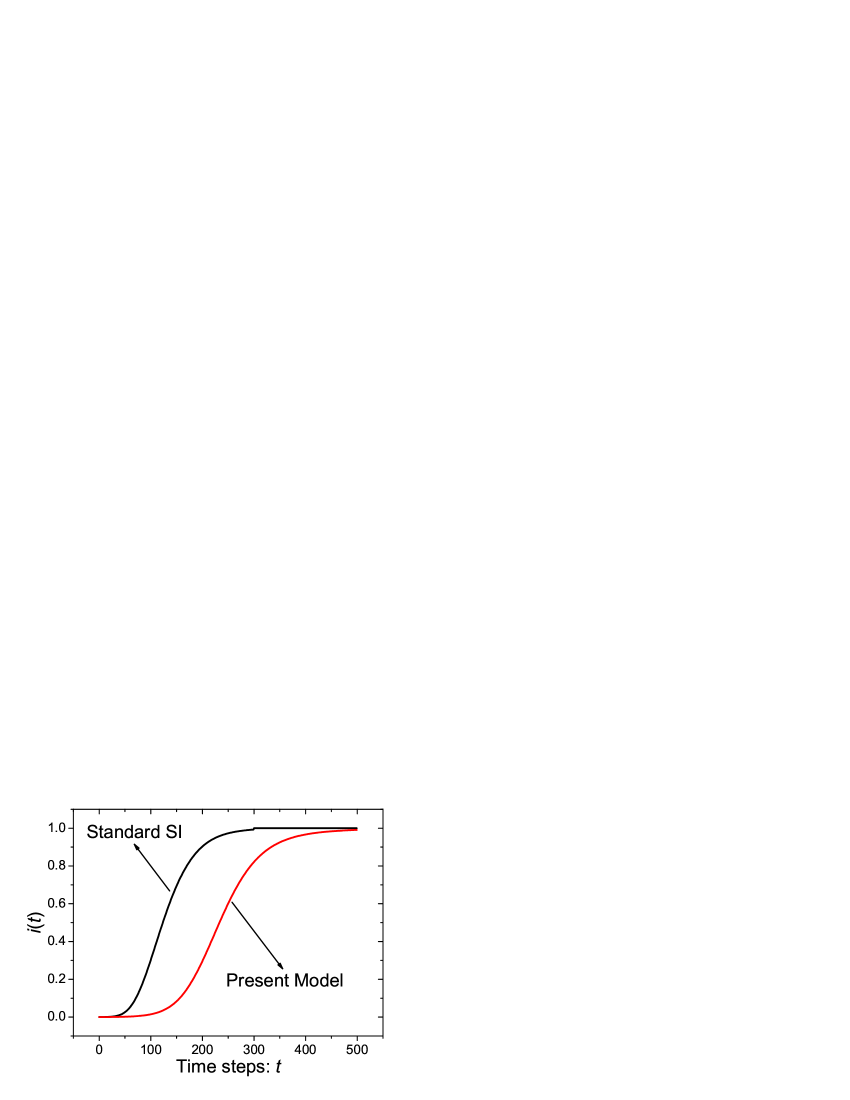
Figure 1: (Color online) The infected density $i(t)$ vs time, where $i(t)=I(t)/N$. The black and red curves result from the standard SI network model and the present model. The numerical simulations are implemented based on the BA network Barabasi1999 of size $N=5000$ and with average degree $\langle k\rangle=6$. The spreading rate is given as $\lambda=0.01$, and the data are averaged over 5000 independent runs.

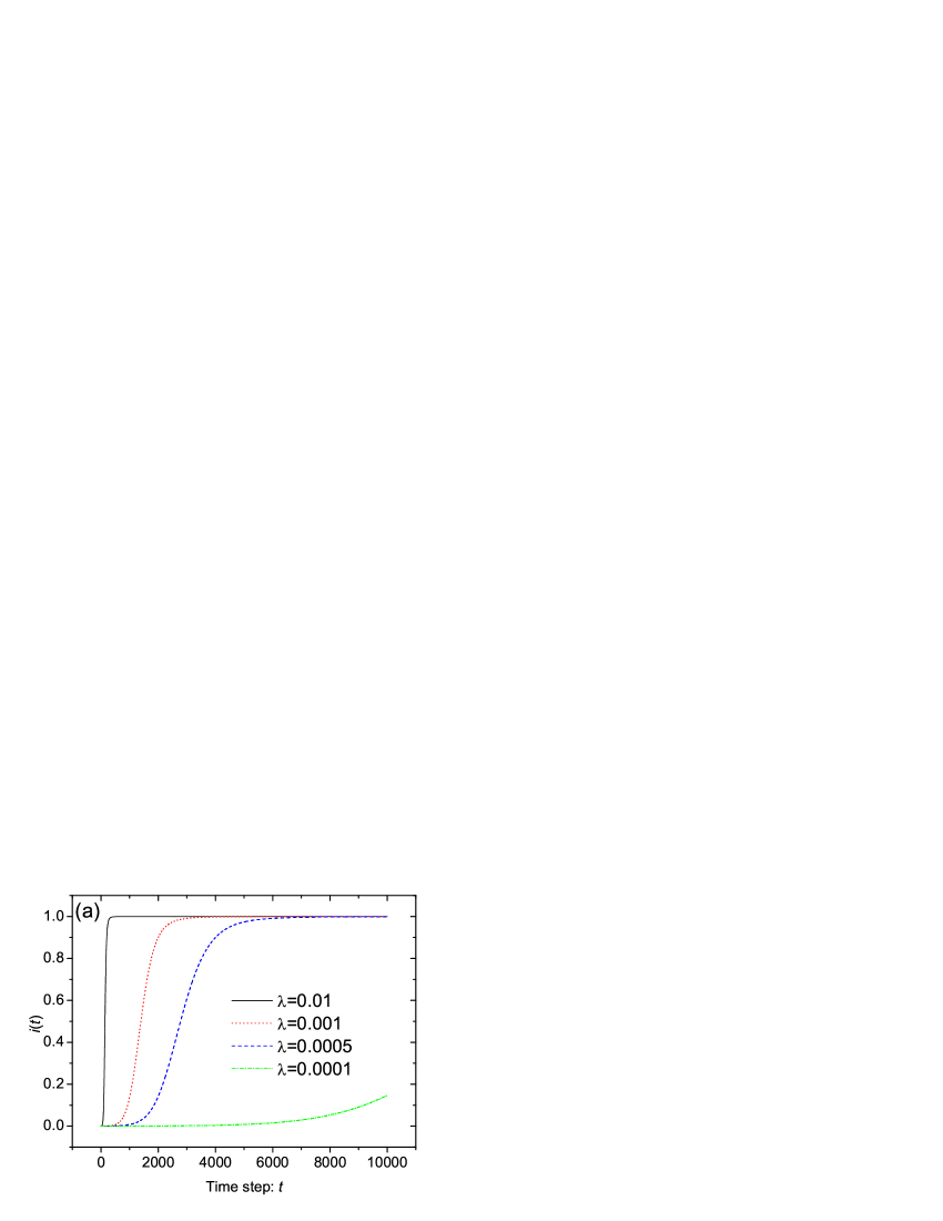
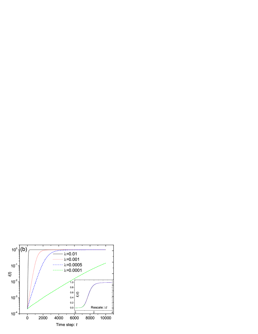
Figure 2: (Color online) The infected density $i(t)$ vs time in normal (a) and single-log (b) plots. The black solid, red dot, green dash and blue dash-dot curves correspond to $\lambda=0.01,0.001,0.0005$ and 0.0001, respectively. In single-log plot (b), the early behavior of $i(t)$ can be well fitted by a straight line, indicating the exponential growth of infected population. The inset shows the rescaled curves $i(\lambda t)$. The four curves for different $\lambda$ collapse to one curve in the new scale $\lambda t$. The numerical simulations are implemented based on a BA network of size $N=5000$ and with average degree $\langle k\rangle=6$, and the data are averaged over 5000 independent runs.

II Model

Different from the previous works, here we investigate the SI process on scale-free networks with identical infectivity. In our model, individuals can be in two discrete states, either susceptible or infected. The total population (i.e. the network size) $N$ is assumed to be constant; thus, if $S(t)$ and $I(t)$ are the numbers of susceptible and infected individuals at time $t$, respectively, then

$$N=S(t)+I(t).$$ (1)

Denote by $\lambda$ the spreading rate at which each susceptible individual acquires infection from an infected neighbor during one time step. Accordingly, one can easily obtain the probability that a susceptible individual $x$ will be infected at time step $t$ to be

$$\lambda_{x}(t)=1-(1-\lambda)^{\theta(x,t-1)},$$ (2)

where $\theta(x,t-1)$ denotes the number of contacts between $x$ and the infected individuals at time $t-1$. For small $\lambda$, one has

$$\lambda_{x}(t)\approx\lambda\theta(x,t-1).$$ (3)

In the standard SI network model Barthelemy2004 ; Barthelemy2005 ; Zhou2005 , each infected individual will contact all its neighbors once at each time step, thus the infectivity of each node is defined by its degree and $\theta(x,t)$ is equal to the number of its infected neighbors at time $t$. In the present model, we assume every individual has the same infectivity $A$, in which, at every time step, each infected individual will generate $A$ contacts where $A$ is a constant. Multiple contacts to one neighbor are allowed, and contacts between two infected ones, although having no effect on the epidemic dynamics, are also counted just like the standard SI model. The dynamical process starts by selecting one node randomly, assuming it is infected.

III Spreading Velocity

In the standard SI network model, the average infectivity equals the average degree $\langle k\rangle$. Therefore, in order to compare the proposed model with the standard one, we set $A=\langle k\rangle$. As shown in Fig. 1, the dynamical behaviors of the present model and the standard one are clearly different: The velocity of the present model is much less than that of the standard model.

In the following discussions, we focus on the proposed model. Without loss of generality, we set $A=1$. Denote by $i_{k}(t)$ the density of infected $k$-degree nodes. Based on the mean-field approximation, one has

$$\frac{\texttt{d}i_{k}(t)}{\texttt{d}t}=\lambda k[1-i_{k}(t)]\sum_{k^{\prime}}\frac{1}{k^{\prime}}\frac{k^{\prime}P(k^{\prime})i_{k^{\prime}}(t)}{\sum_{k^{\prime\prime}}k^{\prime\prime}P(k^{\prime\prime})},$$ (4)

where $P(k)$ denotes the probability that a randomly selected node has degree $k$. The factor $\frac{1}{k^{\prime}}$ accounts for the probability that one of the infected neighbors of a node, with degree $k^{\prime}$, will contact this node at the present time step. Note that the infected density is given by

$$i(t)=\sum_{k}i_{k}(t)P(k),$$ (5)

so Eq. (4) can be rewritten as

$$\frac{\texttt{d}i_{k}(t)}{\texttt{d}t}=\frac{\lambda k}{\langle k\rangle}[1-i_{k}(t)]i(t).$$ (6)

Manipulating the operator $\sum_{k}P(k)$ on both sides, and neglecting terms of order $\mathbb{O}(i^{2})$, one obtains the evolution behavior of $i(t)$ as follows:

$$i(t)\sim\texttt{e}^{ct},$$ (7)

where $c\propto\lambda$ is a constant independent of the power-law exponent $\gamma$.

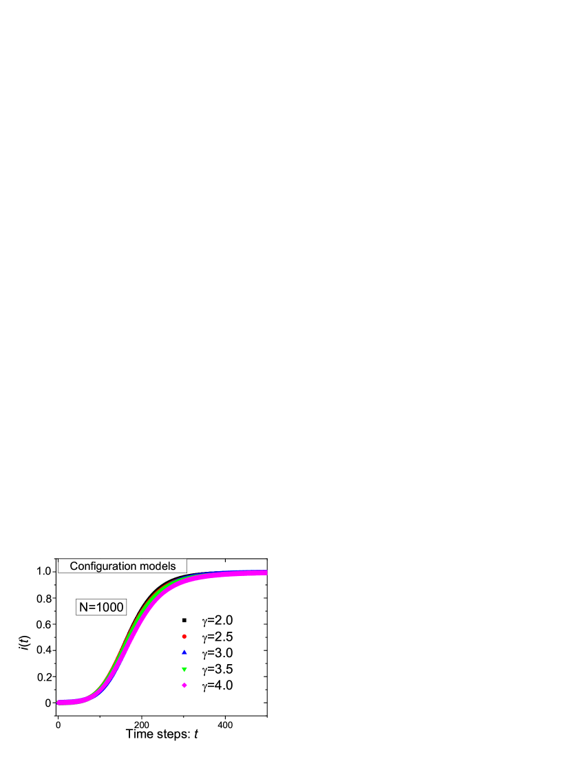
Figure 3: (Color online) The infected density $i(t)$ vs time for different $\gamma$. The black squares, red circles, blue up-triangles, green down-triangles, and pink diamonds (from up to down) denote the cases of $\gamma=2.0,2.5,3.0,3.5$ and 4.0, respectively. The numerical simulations are implemented based on the scale-free configuration network model. The networks are of size $N=1000$ and with average degree $\langle k\rangle=6$, the spreading rate is given as $\lambda=0.01$, and the data are averaged over 10000 independent runs.

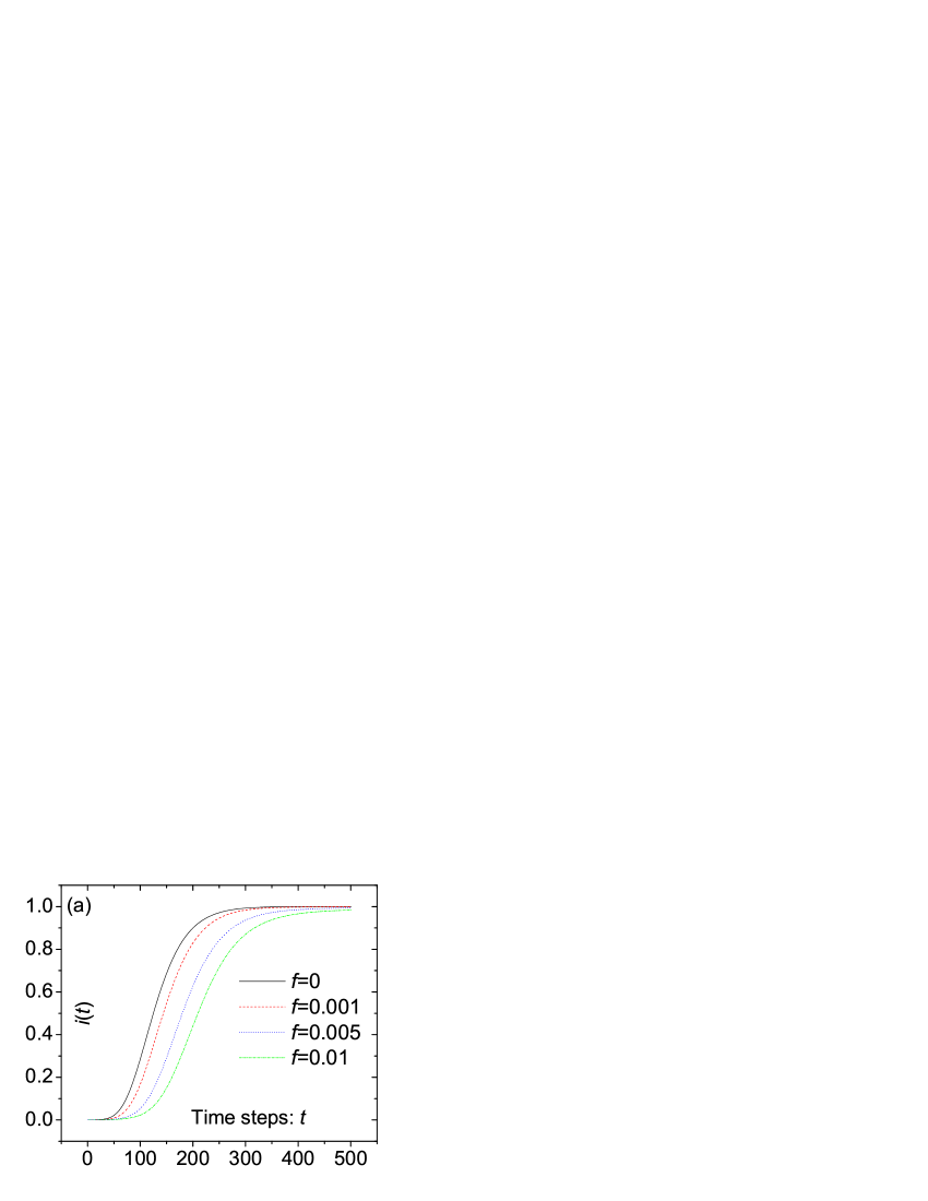
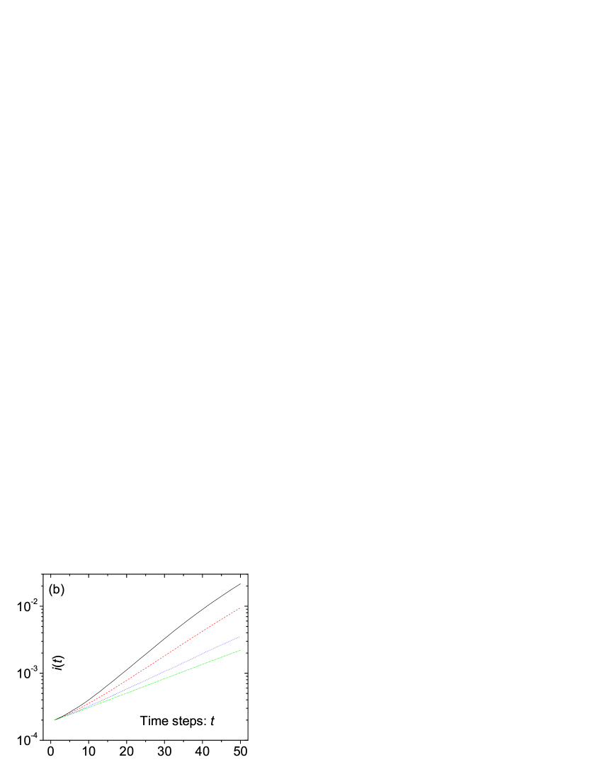
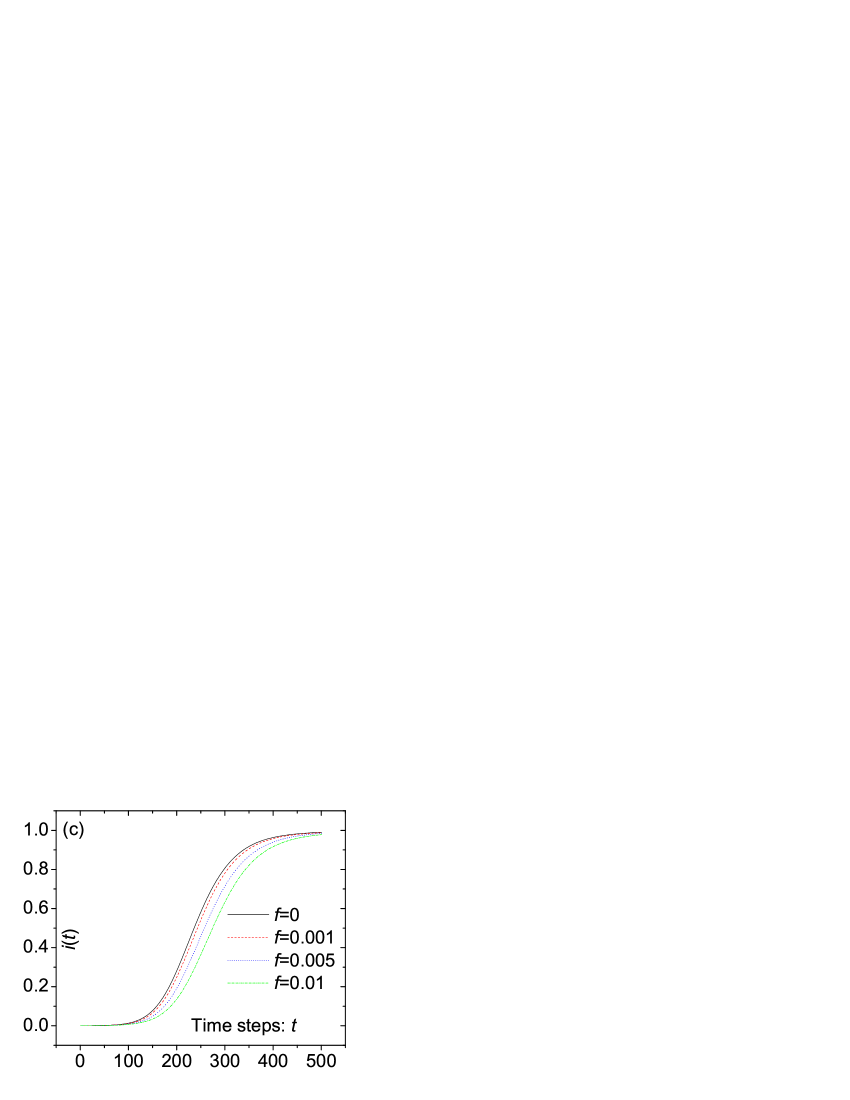
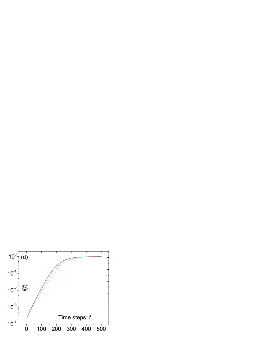
Figure 4: (Color online) The infected density $i(t)$ va time with different vaccinating ranges. Figure 4a and 4b show the results of targeted immunization for the standard SI process in normal and single-log plots, respectively. Correspondingly, figure 4c and 4d display the results for the present model. In all the four panels, the black solid, red dash, blue dot and green dash-dot curves represent the cases of $f=0$, 0.001, 0.005 and 0.01, respectively. The numerical simulations are implemented based on a BA network of size $N=5000$ and with average degree $\langle k\rangle=6$, the spreading rate is given as $\lambda=0.01$, and the data are averaged over 5000 independent runs. For comparison, the infectivity of the present model is set as $A=\langle k\rangle=6$.

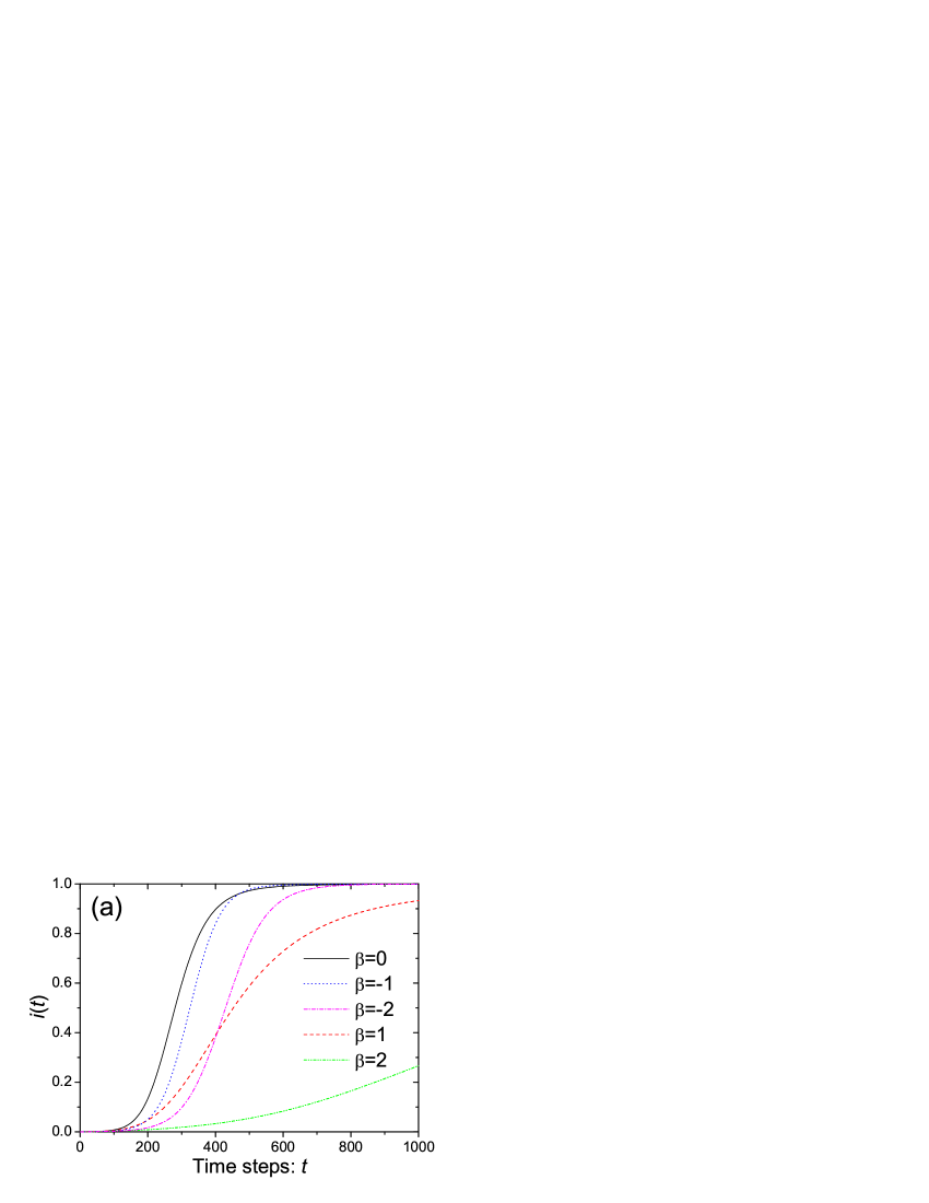
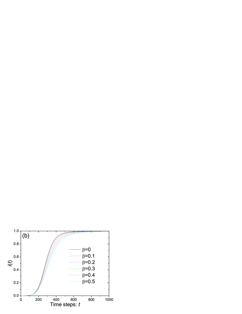
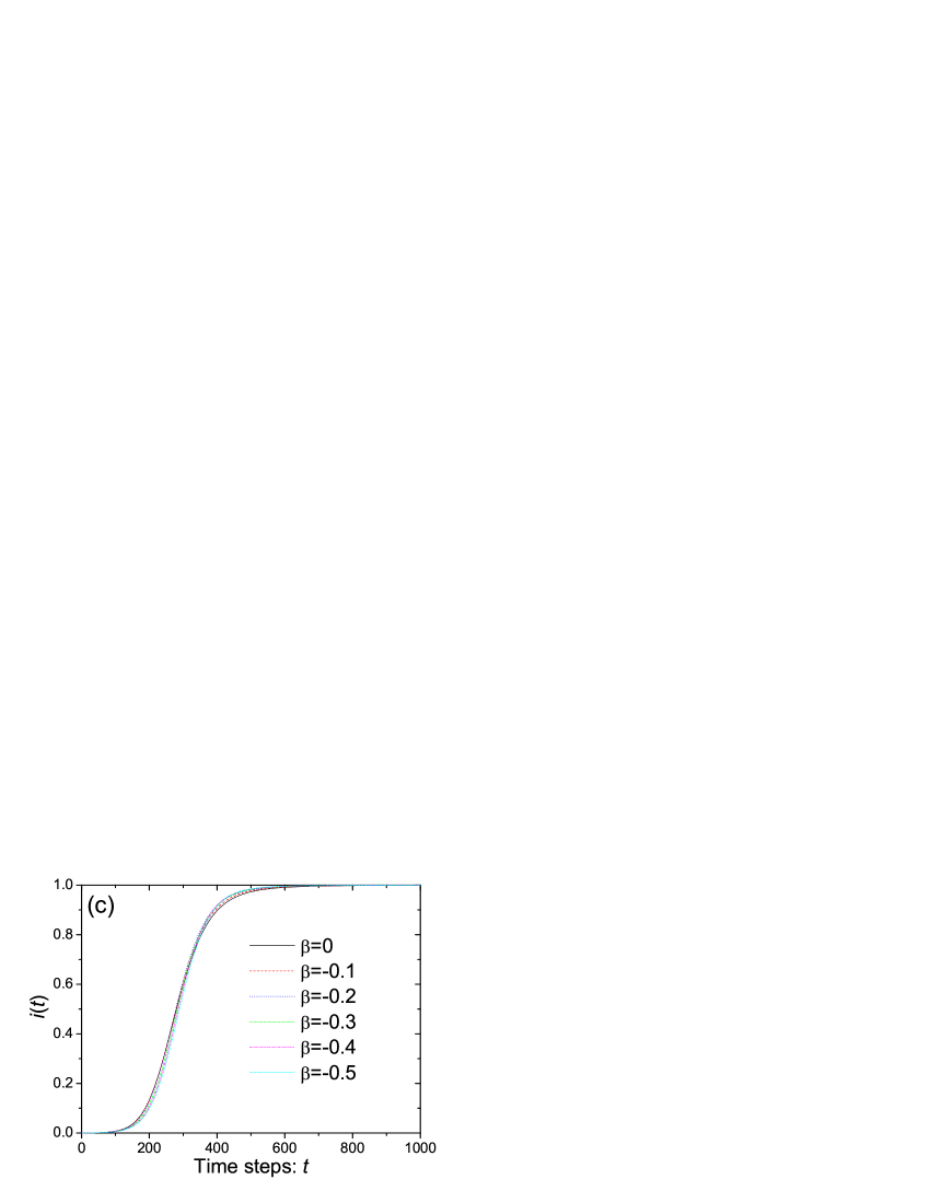
Figure 5: (Color online) The infected density $i(t)$ vs time for different $\beta$. In Figure 5(a), the black solid, blue dot, magenta dash-dot, red dash and green dash-dot-dot curves correspond to $\beta=0$, -1, -2, 1 and 2, respectively. In Figure 5(b), the black solid, red dash, blue dot, green dash-dot, magenta dash-dot-dot and cyan short-dash curves, from up to down, correspond to $\beta=0$, 0.1, 0.2, 0.3, 0.4 and 0.5, respectively. In Figure 5(c), the black solid, red dash, blue dot, green dash-dot, magenta dash-dot-dot and cyan short-dash curves correspond to $\beta=0$, -0.1, -0.2, -0.3, -0.4 and -0.5, respectively. The numerical simulations are implemented based on the extensional BA network of size $N=5000$ and with average degree $\langle k\rangle=6$, the spreading rate is given as $\lambda=0.01$ and the data are averaged over 5000 independent runs.

In Fig. 2, we report the simulation results of the present model for different spreading rates ranging from 0.0001 to 0.01. The curves $i(t)$ vs $t$ can be well fitted by a straight line in single-log plot for small $t$ with slope proportional to $\lambda$ (see also the inset of Fig. 2b, where the curves for different values of $\lambda$ collapse to one curve in the time scale $\lambda t$), which strongly supports the analytical results. Furthermore, based on the scale-free configuration model Newman2001 ; Chung2002 , we investigated the effect of network structure on epidemic behaviors. Different from the standard SI network model Barthelemy2004 ; Barthelemy2005 , which is highly affected by the power-law exponent $\gamma$, as shown in Fig. 3, the exponent $\gamma$ here has almost no effects on the epidemic behaviors of the present model. In other words, in the present model, the spreading rate $\lambda$, rather than the heterogeneity of degree distribution, governs the epidemic behaviors.

IV Targeted Immunization

An interesting and practical problem is whether the epidemic propagation can be effectively controlled by vaccination aiming at part of the population Pastor2003 ; Zhou2006 ; Li2006 . The most simple case is to select some nodes completely randomly, and then vaccinate them. By applying the percolation theory, this case can be exactly solved Cohen2000 ; Callway2000 . The corresponding result shows that it is not an efficient immunization strategy for highly heterogeneous networks such as scale-free networks. Recently, some efficient immunization strategies for scale-free networks are proposed. On the one hand, if the degree of each node can not be known clearly, an efficient strategy is to vaccinate the random neighbors of some randomly selected nodes since the node with larger degree has greater chance to be chosen by this double-random chain than the one with small degree Huerta2002 ; Cohen2003 . On the other hand, if the degree of each node is known, the most efficient immunization strategy is the so-called targeted immunization Pastor2002 ; Madar2004 , wherein the nodes of highest degree are selected to be vaccinated (see also a similar method in Ref. Dezso2002 ).

Here, we compare the performance of the targeted immunization for standard SI model and the present model. To implement this immunization strategy, a fraction of population having highest degree, denoted by $f$, are selected to be vaccinated. That is to say, these $Nf$ nodes will never be infected but the contacts between them and the infected nodes are also counted. Clearly, in both the two models, the hub nodes have more chances to receive contacts from their infected neighbors, thus this targeted immunization strategy must slow down the spreading velocity. In Fig. 4a and Fig. 4b, we report the simulation results for the standard SI model. The spreading velocity remarkably decreases even only a small fraction, $f=0.001$, of population get vaccinated, which strongly indicate the efficiency of the targeted immunization. Relatively, the effect of the targeted immunization for the present model is much weaker (see Fig. 4c and Fig. 4d). The difference is more obvious in the single-log plot (see Fig. 4b and Fig. 4d): The slope of the curve $i(t)\sim t$, which denotes the time scale of the exponential term that governs the epidemic behaviors, sharply decreases even only a small amount of hub nodes are vaccinated in standard SI process while changes slightly in the present model.

V Fast Spreading Strategy

As mentioned in the Sec. 4, previous studies about network epidemic processes focus on how to control the epidemic spreading, especially for scale-free networks. Contrarily, few studies aim at accelerating the epidemic spreading process. However, a fast spreading strategy may be very useful for enhancing the efficiency of network broadcasting or for making profits from network marketing. In this section, we give a primary discussion on this issue by introducing and investigating a simple fast spreading strategy. Since the whole knowledge of network structure may be unavailable for large-scale networks, here we assume only local information is available.

In our strategy, at every time step, each infected node $x$ will contact its neighbor $y$ (in the broadcasting process, it means to forward a message to node $y$) at a probability proportional to $k_{y}^{\beta}$, where $k_{y}$ denotes the degree of $y$. There are two ingredients simultaneously affect the performance of the present strategy. On the one hand, the strategy preferring large-degree node (i.e. the strategy with $\beta>0$) corresponds to shorter average distance in the path searching algorithm Adamic2001 ; Kim2002 , thus it may lead to faster spreading. On the other hand, to contact an already infected node (i.e. to forward a message to a node having already received this message) has no effects on the spreading process, and the nodes with larger degrees are more easily to be infected according to Eq. (6) in the case of $\beta=0$. Therefore, the strategy with $\beta>0$ will bring many redundant contacts that may slow down the spreading. For simplicity, we call the former the shorter path effect (SPE), and the latter the redundant contact effect (RCE).

Figure 5(a) shows the density of infected individuals $i(t)$ as a function of $t$ for different $\beta$. Clearly, due to the competition between the two ingredients, SPE and RCE, the strategies with too large (e.g. $\beta=1,2$) or too small (e.g. $\beta=-1,-2$) $\beta$ are inefficient comparing with the unbiased one with $\beta=0$. The cases when $\beta$ is around zero are shown in Figs. 5(b) and 5(c). In Fig. 5(b), one can see that the RCE plays the major role in determining the epidemic velocity when $\beta>0$; that is, larger $\beta$ leads to slower spreading. As shown in Fig. 5(c), the condition is much more complex when $\beta<0$: In the early stage, the unbiased strategy seems better; however, as time goes on, it is exceeded by the others.

VI Conclusion and Discussion

Almost all the previous studies about the SI model in scale-free networks essentially assume that the nodes of large degrees are not only dominant in topology, but also the superspreaders. However, not all the SI network processes can be appropriately described under this assumption. Typical examples include the network broadcasting process with a limited forwarding capacity, the epidemics of sexually transmitted diseases where all individuals’ sexual activities are pretty much the same due to the physiological limitations, the email service systems with limited ability to accept new clients, the network marketing systems where the referral of products to potential consumers costs money and time, and so on. Inspired by these practical requirements, in this article we have studied the behaviors of susceptible-infected epidemics on scale-free networks with identical infectivity. The infected population grows in an exponential form in the early stage. However, different from the standard SI network model, the epidemic behavior is not sensitive to the power-law exponent $\gamma$, but is governed only by the spreading rate $\lambda$. Both the simulation and analytical results indicate that it is the heterogeneity of infectivities, rather than the heterogeneity of degrees, governs the epidemic behaviors. Further more, we compare the performances of targeted immunization on the standard SI process and the present model. In this standard SI process, the spreading velocity decreases remarkably even only a slight fraction of population are vaccinated. However, since the infectivity of the hub nodes in the present model is just equal to that od the small-degree node, the targeted immunization for the present model is much less efficient.

We have also investigated a fast spreading strategy when only local information is available. Different from previous reports about some relative processes taking place on scale-free networks Adamic2001 ; Kim2002 , we found that the strategy preferring small-degree nodes is more efficient than those preferring large nodes. This result indicates that the redundant contact effect is more important than the shorter path effect. This finding may be useful in practice. Very recently, some authors suggested using a quantity named saturation time to estimate the epidemic efficiency Zhu2004 ; Saramaki2005 , which means the time when the infected density, $i(t)$, firstly exceeds 0.9. Under this criterion, the optimal value of $\beta$ leading to the shortest saturation time is -0.3.

Some recent studies on network traffic dynamics show that the networks will have larger throughput if using routing strategies preferring small-degree nodes Yin2006 ; Wang2006 ; Yan2006 . It is because this strategy can avoid possible congestion occurring at large-degree nodes. Although the quantitative results are far different, there may exist some common features between network traffic and network epidemic. We believe that our work can further enlighten the readers on this interesting subject.

- (1) D. J. Watts, and S. H. Strogatz, Nature 393, 440 (1998).
- (2) A. -L. Barabási, and R. Albert, Science 286, 509 (1999).
- (3) R. Albert, and A. -L. Barabási, Rev. Mod. Phys. 74, 47 (2002).
- (4) S. N. Dorogovtsev, and J. F. F. Mendes, Adv. Phys. 51, 1079 (2002).
- (5) M. E. J. Newman, SIAM Review 45, 167 (2003).
- (6) S. Boccaletti, V. Latora, Y. Moreno, M. Chavez, and D. -U. Hwang, Phys. Rep. 424, 175 (2006).
- (7) R. Pastor-Satorras, and A. Vespignani, Epidemics and immunization in scale-free networks. In: S. Bornholdt, and H. G. Schuster (eds.) Handbook of Graph and Networks, Wiley-VCH, Berlin, 2003.
- (8) T. Zhou, Z. -Q. Fu, and B. -H. Wang, Prog. Nat. Sci. 16, 452 (2006).
- (9) R. Pastor-Satorras, and A. Vespignani, Phys. Rev. Lett. 86, 3200 (2001).
- (10) R. Pastor-Satorras, and A. Vespignani, Phys. Rev. E 63, 066117 (2001).
- (11) R. M. May, and A. L. Lloyd, Phys. Rev. E 64, 066112 (2001).
- (12) Y. Moreno, R. Pastor-Satorras, and A. Vespignani, Eur. Phys. J. B 26, 521 (2002).
- (13) A. S. Tanenbaum, Computer Networks (Prentice Hall Press, 1996).
- (14) W. Krause, J. Scholz, and M. Greiner, Physica A 361, 707 (2006).
- (15) J. Park, and S. Sahni, IEEE Trans. Computers 54, 1081 (2005).
- (16) H. A. Harutyunyan, and B. Shao, J. Parallel & Distributed Computing 66, 68 (2006).
- (17) M. Barthélemy, A. Barrat, R. Pastor-Satorras, and A. Vespignani, Phys. Rev. Lett. 92, 178701 (2004).
- (18) M. Barthélemy, A. Barrat, R. Pastor-Satorras, and A. Vespignani, J. Theor. Biol. 235, 275 (2005).
- (19) T. Zhou, G. Yan, and B. -H. Wang, Phys. Rev. E 71, 046141 (2005).
- (20) Z. -M. Gu, T. Zhou, B. -H. Wang, G. Yan, C. -P. Zhu, and Z. -Q. Fu, Dyn. Contin. Discret. Impuls. Syst. Ser. B-Appl. Algorithm 13, 505 (2006).
- (21) Z. -Z. Zhang, L. -L. Rong, and F. Comellas, Physica A 364, 610 (2006).
- (22) A. Barrat, M. Barthélemy, and A. Vespignani, Phys. Rev. Lett. 92, 228701 (2004).
- (23) A. Barrat, M. Barthélemy, and A. Vespignani, Phys. Rev. E 70, 266149 (2004).
- (24) G. Yan, T. Zhou, J. Wang, Z. -Q. Fu, and B. -H. Wang, Chin. Phys. Lett. 22, 510 (2005).
- (25) A. Vazquez, Phys. Rev. Lett. 96, 038702 (2006).
- (26) S. Bassetti, W. E. Bischoff, and R. J. Sherertz, Emerging Infectious Diseases 11, 637 (2005).
- (27) M. Small, and C. K. Tse, Physica A 351, 499 (2005).
- (28) W. -J. Bai, T. Zhou, and B. -H. Wang, arXiv: physics/0602173.
- (29) P. Gupta, and P. R. Kumar, IEEE Trans. Inf. Theory 46, 388 (2000).
- (30) F. Liljeros, C. R. Rdling, L. A. N. Amaral, H. E. Stanley, and Y. Åberg, Nature 411, 907 (2001).
- (31) F. Liljeros, C. R. Rdling, and L. A. N. Amaral, Microbes and Infection 5, 189 (2003).
- (32) A. Schneeberger, C. H. Mercer, S. A. J. Gregson, N. M. Ferguson, C. A. Nyamukapa, R. M. Anderson, A. M. Johnson, and G. P. Garnett, Sexually Transmitted Diseases 31, 380 (2004).
- (33) See the details about Gmail system from the web site http://mail.google.com/mail/help/intl/en/about.html.
- (34) B. J. Kim, T. Jun, J. Y. Kim, and M. Y. Choi, Physica A 360, 493 (2006).
- (35) M. E. J. Newman, S. H. Strogatz, and D. J. Watts, Phys. Rev. E 64, 026118 (2001).
- (36) F. Chung, and L. Lu, Annals of Combinatorics 6, 125-145 (2002).
- (37) X. Li, and X. -F. Wang, IEEE Trans. Automatic Control 51, 534 (2006).
- (38) R. Cohen, K. Erez, D. ben-Avraham, and S. Havlin, Phys. Rev. Lett. 85, 4626 (2000).
- (39) D. S. Callway, M. E. J. Newman, S. H. Strogatz, and D. J. Watts, Phys. Rev. Lett. 85, 5468 (2000).
- (40) R. Huerta, and L. S. Tsimring, Phys. Rev. E 66, 056115 (2002).
- (41) R. Cohen, S. Havlin, and D. ben-Avraham, Phys. Rev. Lett. 91, 247901 (2003).
- (42) R. Pastor-Satorras, and A. Vespignani, Phys. Rev. E 65, 036104 (2002).
- (43) N. Madar, T. Kalisky, R. Cohen, D. ben-Avraham, and S. Havlin, Eur. Phys. J. B 38, 269 (2004).
- (44) Z. Dezsö, and A. -L. Barabási, Phys. Rev. E 65, 055103 (2002).
- (45) L. A. Adamic, R. M. Lukose, A. R. Puniyani, and B. A. Huberman, Phys. Rev. E 64, 046135 (2001).
- (46) B. -J. Kim, C. N. Yoon, S. K. Han, and H. Jeong, Phys. Rev. E 65, 027103 (2002).
- (47) C. -P. Zhu, S. -J. Xiong, Y. -T. Tian, N. Li, and K. -S. Jiang, Phys. Rev. Lett. 92, 218702 (2004).
- (48) J. Saramaki, and K. Kaski, J. Theor. Biol. 234, 413 (2005).
- (49) C. -Y. Yin, B. -H. Wang, W. -X. Wang, T. Zhou, and H. -J. Yang, Phys. Lett. A 351, 220 (2006).
- (50) W. -X. Wang, B. -H. Wang, C. -Y. Yin, Y. -B. Xie, and T. Zhou, Phys. Rev. E 73, 026111 (2006).
- (51) G. Yan, T. Zhou, B. Hu, Z. -Q. Fu, and B. -H. Wang, Phys. Rev. E 73, 046108 (2006).