Atom interferometer as a selective sensor of rotation or gravity

Abstract

In the presence of Earth gravity and gravity-gradient forces, centrifugal and Coriolis forces caused by the Earth rotation, the phase of the time-domain atom interferometers is calculated with accuracy up to the terms proportional to the fourth degree of the time separation between pulses. We considered double-loop atom interferometers and found appropriate condition to eliminate their sensitivity to acceleration to get atomic gyroscope, or to eliminate the sensitivity to rotation to increase accuracy of the atomic gravimeter. Consequent use of these interferometers allows one to measure all components of the acceleration and rotation frequency projection on the plane perpendicular to gravity acceleration. Atom interference on the Raman transition driving by noncounterpropagating optical fields is proposed to exclude stimulated echo processes which can affect the accuracy of the atomic gyroscopes. Using noncounterpropagating optical fields allows one to get a new type of the Ramsey fringes arising in the unidirectional Raman pulses and therefore centered at the two-quantum line center. Density matrix in the Wigner representation is used to perform calculations. It is shown that in the time between pulses, in the noninertial frame, for atoms with fully quantized spatial degrees of freedom, this density matrix obeys classical Liouville equations.

I Introduction

Since atom interference c1 has been proposed as a sensor of inertial effects c2 and the use of Raman transition between atomic hyperfine sublevels c3 allowed tremendously increase the time separation between optical fields, unprecedented accuracy in the measurement of the Earth rotation c4 , gravity gradients c5 , $\hbar/m_{Cs}$ c6 , and accelerations c7 has also been achieved. The theoretical analysis c71 ; c72 ; c8 ; c9 showed that the current level of interferometer phase measurements is sufficient to sense each source changing the atomic motion, i.e., rotation, acceleration, acceleration gradient, and recoil effect c10 , as well as the interplay between them, such as between rotation and acceleration c8 , recoil effect and rotation c11 , recoil effect and gravity gradientc8 .

At the same time for navigation and geodetic applications one needs to measure separately a gravity acceleration $\mathbf{g}$ and rotation frequency $\mathbf{\Omega},$ i.e., one needs an interferometer whose phase is selectively sensitive only to one component of these vectors, while the sensitivity to others can be either excluded with sufficiently high accuracy or precisely taken into account. An example here is an atomic gyro c4 , where the $\mathbf{\Omega}$ projection on the gravity acceleration $\mathbf{g}$ has been measured, because influence of gravity has been excluded using spatially separated fields propagating in horizontal plane and using signals from two counterpropagating atomic beams.

In this article we consider the theory of atom interferometers that would allow one to measure separately an atom acceleration $\mathbf{g}$ and the rotation frequency component $\mathbf{\Omega}$ which are perpendicular to $\mathbf{g}.$ We explore the fact that, when rotation, gravity gradient and recoil effect only slightly affect the atoms’ trajectory, parts of the interferometer phase associated with $\mathbf{g}$ and $\mathbf{\Omega}$ evolve correspondingly as $T^{2}$ and $T^{3}$ while other contributions are precisely known or negligibly small. Using particular kinds of the atom interferometers one can exclude one of these dependences getting a sensor of acceleration or rotation only.

Usual time domain atom interferometer, consisting of three resonant pulses applied to the cold atom cloud at moments $t=0,$ $T_{2}$ and $T_{3}$ could not serve for these purposes because the only parameter, ratio of the time separation between pulses $T_{3}/T_{2}$, is already used to eliminate linear in time part of the phase. This Doppler phase vanishes at the echo point, $T_{3}=2T_{2}.$ To eliminate another terms one needs at least a four-pulse interferometer. It was found previously c2 ; c121 ; c13 that double loop interferometer consisting of two $\pi/2$ pulses at the beginning and end and two $\pi$ pulses in between, i.e., the $\left(\pi/2,T_{1}=0\right)-\left(\pi,T_{2}\right)-\left(\pi,T_{3}\right)-\left(\pi/2,T_{4}\right)$ interferometer, has no sensitivity to the homogeneous acceleration if $T_{2}=\dfrac{1}{4}T_{4}$ and $T_{3}=\dfrac{3}{4}T_{4},$ see fig. 1(a).

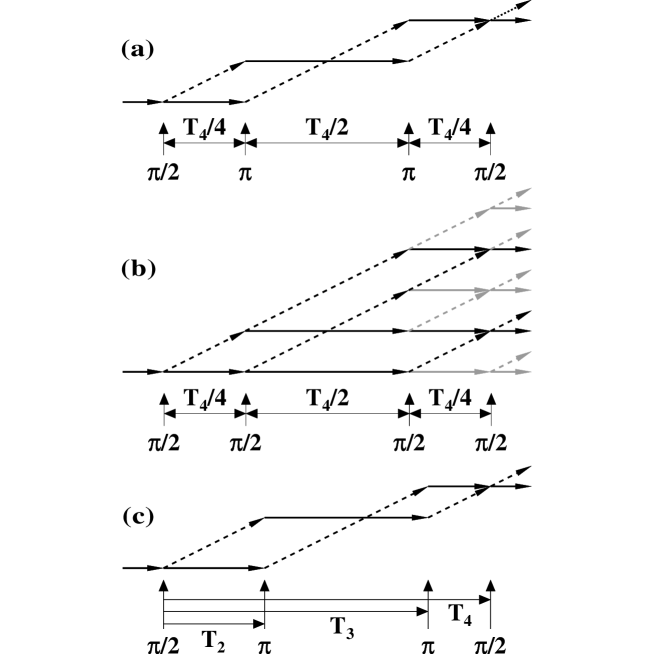
Figure 1: Recoil diagrams for four-pulse atom interferometers, $\left(a\right)$ double-loop interferometer insensitive to homogeneous acceleration; $\left(b\right)$ stimulated echo processes, shown by black parallelograms, which could restore sensitivity to acceleration; $\left(c\right)$ double-loop interferometer with nonidentical loops, $T_{2,3}=\dfrac{\sqrt{5}\mp 1}{4}T_{4}.$ Solid and dashed lines correspond to the lower and upper atomic states.

One can expect that the double-loop interferometer can serve as a sensor of rotation. It is correct only if pulses’ areas are precisely equal to assigned values. If one could not hold areas equal to $\pi$ or $\pi/2,$ then stimulated echo processes also contribute [see Fig. 1(b)] to the interferometer phase and since stimulated echo is insensitive to the atomic motion between second and third pulses, their contribution is acceleration sensitive. Since typically contribution to the interferometers phase caused by the acceleration is 5-6 orders of magnitude larger than that caused by rotation c121 , it is extremely important to find a technique for excluding stimulated echo. To achieve this goal one should violate the condition for stimulated echo. This opportunity exists if one uses Raman transitions, where the splitting of atomic momentum states  occurs under the action of two optical fields having wave vectors $\mathbf{q}_{1}$ and $\mathbf{q}_{2},$ such as an effective wave vector associated with Raman transition is given by $\mathbf{k}=\mathbf{q}_{1}-\mathbf{q}_{2}.$ In principle one can use for this purpose noncouterpropagating fields. Interferometers with $\mathbf{q}_{1}\not=-\mathbf{q}_{2}$ have been previously created c131 and studied c132 .

Since for Raman transition between hyperfine sublevels $q_{1}\approx q_{2},$ $\left|\mathbf{k}\right|\approx k\sin\alpha,$ where $\alpha$ is the half-angle between vectors $\mathbf{q}_{1}$ and $\mathbf{q}_{2},$ and $k\approx 2q_{1}$ is the maximum value of the effective wave vector corresponding to counterpropagating optical fields. If $\mathbf{k}_{j}$ is an effective wave vector associated with Raman pulse $j,$ than the phase matching condition for pulse sequences $\pi/2-\pi-\pi-\pi/2$ [Fig. 1(a)] and $\pi/2-\pi/2-\pi/2-\pi/2$ [Fig. 1(b)] are

$$\mathbf{k}_{4}-2\mathbf{k}_{3}+2\mathbf{k}_{2}-\mathbf{k}_{1}=0,$$ (1a)

$$\mathbf{k}_{4}-\mathbf{k}_{3}-\mathbf{k}_{2}+\mathbf{k}_{1}=0.$$ (1b)

These conditions mean the same only for parallel pulses having effective wave vectors of the same absolute values $k_{j}$. But even for pulses with slightly different $k_{j}$ one can hold only one of this condition and violate another. In this paper we propose and analyze an exclusion of the stimulated echo processes using for double loop atom interferometers Raman pulses with nonequal effective wave vectors.

While eliminating $T^{2}$ dependences one can use time domain interferometer as a gyroscope, to measure rotation frequency components perpendicular to acceleration, eliminating $T^{3}$ dependences would guarantee that contributions of this order, which can be caused by c8 gravity gradient (for atoms with nonzero launch momentum), rotation (when effective wave  vectors are not parallel to the acceleration), recoil effect and combinations of these factors, do not affect the interferometer phase at all. Absence of $T^{3}$ dependences should increase the accuracy of the acceleration measurement. We will show below that $T^{3}$ dependences disappear for the double-loop interferometer with nonidentical loops shown in Fig. 1(c). Since in this case pulse separations $T_{2},$ $T_{3}$ and $T_{4}$ are incommensurate, one can be sure that no other echolike processes can affect the interferometer phase.

In this paper we perform calculations of interferometers’ phases for three- and four-pulse cases, for arbitrarily directed gravity acceleration and rotation including Earth gravity gradient as a small correction. It would allow us to get the phases’ terms evolving up to $T^{4}$ dependences. In our calculation we use equations for the density matrix in the Wigner representation, which are convenient to describe atomic clouds’ evolution between pulses c14 , because we show that in this representation density matrix evolves exactly as the classical distribution function in the rotating frame in the presence of the homogeneous gravity and gravity gradient terms. This technique is mathematically equivalent to the pure quantum consideration of the atomic wave function evolution in the space between pulses elaborated in c72 .

Using density matrix in the Wigner representation allows us to evaluate precisely all effects related to the atomic spatial motion quantization without calculating path integrals c15 .

The paper is arranged as follows. A simplified consideration of four-pulse interferometer is performed in Sec. II. Evolution of the density matrix in the Wigner representation is considered in Sec. III. Atom trajectory in the Earth rotating frame, including gravity-gradient terms as perturbation, is calculated in Sec. IV. Density matrix jumps under the pulse action are obtained in Sec. V. In Sec. VI we calculate the phase of the $\pi/2-\pi-\pi/2$ pulse interferometer. Section VII is devoted to study four-pulse interferometers as atomic gyroscope or gravimeter, while in Sec. VIII we summarize our consideration and discuss further possible developments of the proposed multiple loop interferometers technique.

II Four-pulse atom interferometers

Consider an interaction of cold atoms with a sequence of four Raman pulses, $\pi/2-\pi-\pi-\pi/2,$ having the same effective wave vector $\mathbf{k}$ and applied at moments $T_{1}=0,$ $T_{2}$, $T_{3},$ and $T_{4}.$ We will show below that for atoms with initial coordinate and momentum $\mathbf{r}$ and $\mathbf{p}$ the phase of interferometer associated with atomic motion is given by

$$\phi_{m}=\mathbf{k}\cdot\left[\mathbf{R}\left(\mathbf{r},\mathbf{p}+\dfrac{\hbar\mathbf{k}}{2},T_{4}\right)-2\mathbf{R}\left(\mathbf{r},\mathbf{p}+\dfrac{\hbar\mathbf{k}}{2},T_{3}\right)+2\mathbf{R}\left(\mathbf{r},\mathbf{p}+\dfrac{\hbar\mathbf{k}}{2},T_{2}\right)-\mathbf{r}\right],$$ (2)

where the function $\mathbf{R}\left(\mathbf{r},\mathbf{p},t\right)$ is the position of an atom at the moment $t$ under the classical motion in rotating frame. For small rotation frequency $\mathbf{\Omega}$ $\left(\Omega t\ll 1\right)$ the atom trajectory is given by

$$\mathbf{R}\left(\mathbf{r},\mathbf{p},t\right)\approx\mathbf{r}+\dfrac{\mathbf{p}}{m}t+\mathbf{g}\dfrac{t^{2}}{2}-\mathbf{\Omega}\times\left(\mathbf{r}+\dfrac{\mathbf{p}}{m}t+\mathbf{g}\dfrac{t^{2}}{3}\right)t,$$ (3)

where $m$ is the atomic mass, and for the phase (2) one arrives at the expression

$$\phi_{m} =\mathbf{k}\cdot\left(\dfrac{\mathbf{p}+\dfrac{\hbar\mathbf{k}}{2}}{m}-\mathbf{\Omega}\times\mathbf{r}\right)T_{4}\left(1-2t_{3}+2t_{2}\right)$$

$$+\mathbf{k}\cdot\left(\dfrac{\mathbf{g}}{2}-\mathbf{\Omega}\times\dfrac{\mathbf{p}}{m}\right)T_{4}^{2}\left(1-2t_{3}^{2}+2t_{2}^{2}\right)$$

$$+\dfrac{1}{3}\left(\mathbf{k}\times\mathbf{g}\right)\cdot\mathbf{\Omega}T_{4}^{3}\left(1-2t_{3}^{3}+2t_{2}^{3}\right),$$ (4)

where

$$t_{j}=T_{j}/T_{4}.$$ (5)

If the purpose is to measure the rotation frequency, then one may set to $0$ first and second terms in Eq. (4). System

$$1-2t_{3}+2t_{2} =0,$$ (6a)

$$1-2t_{3}^{2}+2t_{2}^{2} =0$$ (6b)

has a solution $t_{2}=1/4,t_{3}=3/4$ corresponding to the double loop interferometer c2 ; c121 ; c13 shown in Fig. 1(a). In this case

$$\phi_{m}=\dfrac{1}{16}\left(\mathbf{k}\times\mathbf{g}\right)\cdot\mathbf{\Omega}T_{4}^{3}.$$ (7)

If the gravity is measured, then the phase (7) can be used to measure perpendicular to gravity components of the rotation frequency. For example, for Cs interferometer having the effective wavelength $426~{}$nm and total time separation between pulses $T_{4}=0.8$ s, at the latitude 41^∘ the maximum value of the phase (7) $\phi_{m}\approx 250.$

If the purpose is to eliminate cubic terms in order to increase the accuracy of the acceleration measurement, one should choose the solution of the system

$$1-2t_{3}+2t_{2} =0,$$ (8a)

$$1-2t_{3}^{3}+2t_{2}^{3} =0,$$ (8b)

which is

$$t_{2,3}=\dfrac{\sqrt{5}\mp 1}{4},$$ (9)

and for atoms having zero launch momentum, $\mathbf{p=0,}$ the phase is given by

$$\phi_{m}=-\dfrac{\sqrt{5}-2}{4}\mathbf{k}\cdot\mathbf{g}T_{4}^{2}.$$ (10)

For a given maximum separation between pulses, the absolute value of the phase (10) is approximately $4.2$ times less than the signal in the usual three-pulse interferometer. Therefore, it is a kind of trade off, when one should decide whether it is more important to get a larger signal or to eliminate $T^{3}$ corrections to the phase.

III Density matrix evolution in the free space

Starting with the Lagrangian for an atom in the frame rotating with constant rate,

$$L=\dfrac{m\mathbf{v}^{2}}{2}+m\mathbf{v}\cdot\left(\mathbf{\Omega}\times\mathbf{r}\right)+\dfrac{m}{2}\left(\mathbf{\Omega}\times\mathbf{r}\right)^{2}-U,$$ (11)

where $U$ is the potential, one gets the generalized momentum and Hamiltonian,

$$\mathbf{p} =m\mathbf{v}+m\left(\mathbf{\Omega}\times\mathbf{r}\right);$$ (12a)

$$H =\dfrac{\mathbf{p}^{2}}{2m}+\mathbf{p\cdot}\left(\mathbf{r}\times\mathbf{\Omega}\right)+U.$$ (12b)

In the space free of the laser field, i.e., free space, the density matrix in the Wigner representation c151

$$\rho\left(\mathbf{r},\mathbf{p},t\right)=\dfrac{1}{\left(2\pi\hbar\right)^{3}}\int d\mathbf{s}\rho\left(\mathbf{r}+\dfrac{1}{2}\mathbf{s},\mathbf{r}-\dfrac{1}{2}\mathbf{s},t\right)\exp\left(-i\mathbf{p}\cdot\mathbf{s}/\hbar\right),$$ (13)

where

$$\rho\left(\mathbf{r},\mathbf{r}^{\prime}\right)=\psi\left(\mathbf{r}\right)\otimes\psi^{{\dagger}}\left(\mathbf{r}^{\prime}\right)$$ (14)

is the density matrix in the coordinate representation, evolves as

$$\partial_{t}\rho\left(\mathbf{r},\mathbf{p},t\right) =\dfrac{1}{i\hbar\left(2\pi\hbar\right)^{3}}\int d\mathbf{s}\exp\left(-i\mathbf{p}\cdot\mathbf{s}/\hbar\right)\left\{\left[-\dfrac{\hbar^{2}}{2m}\partial_{\mathbf{r}_{1}}^{2}+i\hbar\partial_{\mathbf{r}_{1}}\left(\mathbf{\Omega}\times\mathbf{r}_{1}\right)+U\left(\mathbf{r}_{1}\right)\right.\right.$$

$$+\left.\left.\dfrac{\hbar^{2}}{2m}\partial_{\mathbf{r}_{2}}^{2}+i\hbar\partial_{\mathbf{r}_{2}}\left(\mathbf{\Omega}\times\mathbf{r}_{2}\right)-U\left(\mathbf{r}_{2}\right)\right]\rho\left(\mathbf{r}_{1},\mathbf{r}_{2},t\right)\right\}_{\mathbf{r}_{1}=\mathbf{r}+\frac{1}{2}\mathbf{s},\mathbf{r}_{2}=\mathbf{r}-\frac{1}{2}\mathbf{s}}.$$ (15)

Using the fact that

$$\partial_{\mathbf{r}_{1}} =\dfrac{1}{2}\partial_{\mathbf{r}}+\partial_{\mathbf{s}};$$

$$\partial_{\mathbf{r}_{2}} =\dfrac{1}{2}\partial_{\mathbf{r}}-\partial_{\mathbf{s}}$$ (16)

and replacing $\partial_{\mathbf{s}}\Rightarrow i\mathbf{p}/\hbar,$ one arrives at equations

$$\left\{\partial_{t}+\left(\dfrac{\mathbf{p}}{m}+\mathbf{r}\times\Omega\right)\partial_{\mathbf{r}}+\left[\left(\mathbf{p}\times\Omega\right)-\partial_{\mathbf{r}}U\right]\partial_{\mathbf{p}}+Q\right\}\rho\left(\mathbf{r},\mathbf{p},t\right)=0;$$ (17a)

$$Q=-\left(i\hbar\right)^{-1}\left[U\left(\mathbf{r}+\dfrac{1}{2}i\hbar\partial_{\mathbf{p}}\right)-U\left(\mathbf{r}-\dfrac{1}{2}i\hbar\partial_{\mathbf{p}}\right)\right]+\partial_{\mathbf{r}}U\partial_{\mathbf{p}}.$$ (17b)

When the potential $U$ is not higher than bilinear function of coordinates, quantum term disappears, $Q=0.$ Since the Hamiltonian equation for the classical momentum and coordinate is

$$\mathbf{\dot{r}} =\dfrac{\mathbf{p}}{m}+\mathbf{r}\times\mathbf{\Omega};$$ (18a)

$$\mathbf{\dot{p}} =-\partial_{\mathbf{r}}U+\left(\mathbf{p}\times\mathbf{\Omega}\right),$$ (18b)

one concludes that, if

$$Q\sim\hbar^{2}\left(\partial_{\mathbf{r}}^{3}U\right)\partial_{\mathbf{p}}^{3}\ll T^{-1},$$ (19)

where $T$ is a typical time of the system’s evolution, then with an accuracy $QT$ the quantum density matrix in the Wigner representation obeys the same equation as the classical density matrix

$$\left(\partial_{t}+\mathbf{\dot{r}}\partial_{\mathbf{r}}+\mathbf{\dot{p}}\partial_{\mathbf{p}}\right)\rho\left(\mathbf{r},\mathbf{p},t\right)=0.$$ (20)

If the density matrix is known at some previous moment $t^{\prime}<t$ then the solution of Eq. (20) is given by

$$\rho\left(\mathbf{r},\mathbf{p},t\right)=\rho\left[\mathbf{R}\left(\mathbf{r},\mathbf{p},t^{\prime}-t\right),\mathbf{P}\left(\mathbf{r},\mathbf{p},t^{\prime}-t\right),t^{\prime}\right],$$ (21)

where functions $\mathbf{R}\left(\mathbf{r}_{0},\mathbf{p}_{0},t\right),\mathbf{P}\left(\mathbf{r}_{0},\mathbf{p}_{0},t\right)$ are solutions of Eqs. (18) subjected to the initial condition $\left(\mathbf{r},\mathbf{p}\right)_{t=0}=\left(\mathbf{r}_{0},\mathbf{p}_{0}\right).$ Clearly these functions have to satisfy multiplication law

$$\mathbf{R}\left[\mathbf{R}\left(\mathbf{r},\mathbf{p},t_{1}\right),\mathbf{P}\left(\mathbf{r},\mathbf{p},t_{1}\right),t_{2}\right] =\mathbf{R}\left(\mathbf{r},\mathbf{p},t_{1}+t_{2}\right),$$ (22a)

$$\mathbf{P}\left[\mathbf{R}\left(\mathbf{r},\mathbf{p},t_{1}\right),\mathbf{P}\left(\mathbf{r},\mathbf{p},t_{1}\right),t_{2}\right] =\mathbf{P}\left(\mathbf{r},\mathbf{p},t_{1}+t_{2}\right).$$ (22b)

Solution (21) is the consequence of the phase-space invariance in time. This is correct only for canonical variables $\left(\mathbf{r},\mathbf{p}\right)$ and incorrect for variables $\left(\mathbf{r},\mathbf{v}\right).$ Solution (21) can be proved as follows

$$\dfrac{\partial\rho\left(\mathbf{r},\mathbf{p},t\right)}{\partial t}=\dfrac{\partial\rho}{\partial R_{i}}\dfrac{dR_{i}\left(\mathbf{r},\mathbf{p},t^{\prime}-t\right)}{dt}+\dfrac{\partial\rho}{\partial P_{i}}\dfrac{dP_{i}\left(\mathbf{r},\mathbf{p},t^{\prime}-t\right)}{dt}.$$ (23)

Since

$$\dfrac{dR_{i}\left(\mathbf{r},\mathbf{p},t^{\prime}-t\right)}{dt}=-\dfrac{dR_{i}\left(\mathbf{r},\mathbf{p},t^{\prime}-t\right)}{dt^{\prime}}=-\dfrac{\partial H}{\partial P_{i}}$$ (24)

and

$$\dfrac{dP_{i}\left(\mathbf{r},\mathbf{p},t^{\prime}-t\right)}{dt}=-\dfrac{dP_{i}\left(\mathbf{r},\mathbf{p},t^{\prime}-t\right)}{dt^{\prime}}=\dfrac{\partial H}{\partial R_{i}},$$ (25)

one gets

$$\dfrac{\partial\rho\left(\mathbf{r},\mathbf{p},t\right)}{\partial t}=-\left\{H,\rho\right\}_{\mathbf{R},\mathbf{P}},$$ (26)

where $\left\{H,\rho\right\}$ is a Poisson bracket, and using invariance of the Poisson brackets $\left\{H,\rho\right\}_{\mathbf{RP}}=\left\{H,\rho\right\}_{\mathbf{rp}}$ one arrives at Eq. (20).

IV Atom classical motion in the rotating frame

In this section we calculate the atomic classical trajectory in the potential consisting of the linear part and gravity gradient part

$$U\left(\mathbf{r}\right) =-m\mathbf{a}\cdot\mathbf{r}+\delta U\left(\mathbf{r}\right),$$ (27a)

$$\delta U\left(\mathbf{r}\right) =\dfrac{m}{4}T_{zz}\left[r^{2}-3\left(\mathbf{n}\cdot\mathbf{r}\right)^{2}\right],$$ (27b)

where $\mathbf{a}=\mathbf{g}-\Omega^{2}R$$\boldsymbol{\nu}$$\times\left(\boldsymbol{\nu}\times\mathbf{n}\right)$ is a sum of the gravity and centrifugal accelerations, $\mathbf{\nu=\Omega}/\Omega$ is a unit vector along the rotation frequency, $\mathbf{n=R}/R$ is a unit vector along the system’s displacement $\mathbf{R}$ from the Earth center, $T_{zz}=-2g_{z}/R,$ $g_{z}$ is the vertical component of the gravity acceleration.

We will treat the gradient term (27b) as a perturbation. In the zero order the atom evolves as

$$\mathbf{\dot{r}} =\mathbf{r}\times\mathbf{\Omega}+\dfrac{\mathbf{p}}{m},$$ (28a)

$$\mathbf{\dot{p}} \mathbf{=}\left(\mathbf{p}\times\Omega\right)+m\mathbf{a},$$ (28b)

subject to initial conditions $\mathbf{r}\left(0\right)=\mathbf{r}_{0},$ $\mathbf{p}\left(0\right)=\mathbf{p}_{0},$ while first-order corrections are given by

$$\delta\mathbf{p} =-\dfrac{m}{2}T_{zz}\mathbf{p}_{\gamma},$$ (29a)

$$\delta\mathbf{r} =-\dfrac{1}{2}T_{zz}\mathbf{r}_{\gamma},$$ (29b)

where $\mathbf{r}_{\gamma}$ and $\mathbf{p}_{\gamma}$ evolve as

$$\mathbf{\dot{r}}_{\gamma} =\mathbf{r}_{\gamma}\times\mathbf{\Omega}+\mathbf{p}_{\gamma},$$ (30a)

$$\mathbf{\dot{p}}_{\gamma} =\mathbf{p}_{\gamma}\times\mathbf{\Omega+r}-3\mathbf{n}\left(\mathbf{n}\cdot\mathbf{r}\right),$$ (30b)

subject to initial conditions $\mathbf{r}_{\gamma}\left(0\right)=0,$ $\mathbf{p}_{\gamma}\left(0\right)=0.$

One sees that to get the atom trajectory it is necessary to solve equations of the type

$$\mathbf{\dot{b}}=\Omega\mathbf{b}\times\boldsymbol{\nu}+\mathbf{f}\left(t\right).$$ (31)

Directing temporarily $z$ axis along $\boldsymbol{\nu,}$ one finds that variable $\xi=b_{x}-ib_{y}$ is given by

$$\xi=\exp\left(i\Omega t\right)\xi_{0}+\int_{0}^{t}d\tau\exp\left[i\Omega\left(t-\tau\right)\right]\left[f_{x}\left(\tau\right)-if_{y}\left(\tau\right)\right],$$ (32)

so that the solution of Eq. (31) can be found as

$$\mathbf{b}=\cos\Omega t\left(b_{0x},b_{0y},0\right)+\sin\Omega t\left(b_{0y},-b_{0x},0\right)$$

$$+\int_{0}^{t}d\tau\left\{\cos\Omega\left(t-\tau\right)\left[f_{x}\left(\tau\right),f_{y}\left(\tau\right),0\right]+\sin\Omega\left(t-\tau\right)\left[f_{y}\left(\tau\right),-f_{x}\left(\tau\right),0\right]\right\}+\left[0,0,b_{0z}+\int_{0}^{t}d\tau f_{z}\left(\tau\right)\right].$$ (33)

Since for the chosen coordinate system $\left(b_{0x},b_{0y},0\right)=-$$\boldsymbol{\nu}$$\times\left(\boldsymbol{\nu}\times\mathbf{b}\right)$ and $\left(b_{0y},-b_{0x},0\right)=-$$\boldsymbol{\nu}$$\times\mathbf{b,}$ then in the vector representation the solution of Eq. (31) is given by

$$\mathbf{b} =\mathbf{b}_{h}+\mathbf{b}_{p},$$ (34a)

$$\mathbf{b}_{h} =-\boldsymbol{\nu}\times\left(\boldsymbol{\nu}\times\mathbf{b}_{0}\cos\Omega t+\mathbf{b}_{0}\sin\Omega t\right)+\boldsymbol{\nu}\left(\boldsymbol{\nu}\cdot\mathbf{b}_{0}\right),$$ (34b)

$$\mathbf{b}_{p} =\int_{0}^{t}d\tau\left\{-\boldsymbol{\nu}\times\left[\boldsymbol{\nu}\times\mathbf{f}\left(\tau\right)\cos\Omega\left(t-\tau\right)+\mathbf{f}\left(\tau\right)\sin\Omega\left(t-\tau\right)\right]+\boldsymbol{\nu}\left[\boldsymbol{\nu}\cdot\mathbf{f}\left(\tau\right)\right]\right\}.$$ (34c)

If in turn the driving term in Eq. (31) can be represented as

$$\mathbf{f}\left(\tau\right)=\boldsymbol{\nu}\times\left[\boldsymbol{\nu}\times\mathbf{s}q_{1}\left(\tau\right)+\mathbf{s}q_{2}\left(\tau\right)\right]+\boldsymbol{\nu}\left(\boldsymbol{\nu}\cdot\mathbf{s}\right)q_{0}\left(\tau\right),$$ (35)

then

$$\mathbf{b}_{p} =\boldsymbol{\nu}\times\left\{\boldsymbol{\nu}\times\int_{0}^{t}d\tau\mathbf{s}\left[q_{1}\left(\tau\right)\cos\Omega\left(t-\tau\right)-q_{2}\left(\tau\right)\sin\Omega\left(t-\tau\right)\right]\right.$$

$$+\left.\int_{0}^{t}d\tau\mathbf{s}\left[q_{1}\left(\tau\right)\sin\Omega\left(t-\tau\right)+q_{2}\left(\tau\right)\cos\Omega\left(t-\tau\right)\right]\right\}+\boldsymbol{\nu}\int_{0}^{t}d\tau\left(\boldsymbol{\nu}\cdot\mathbf{s}\right)q_{0}\left(\tau\right).$$ (36)

Consecutive application of Eqs. (34)-(36) brought us to the following expression for the function $\mathbf{R}\left(\mathbf{r,p},t\right)$

$$\mathbf{R}\left(\mathbf{r},\mathbf{p},t\right)=\mathbf{R}_{0}\left(\mathbf{r},\mathbf{p},t\right)+\delta\mathbf{R}\left(\mathbf{r},\mathbf{p},t\right);$$ (37a)

$$\mathbf{R}_{0}\left(\mathbf{r},\mathbf{p},t\right) =\cos x\left(\mathbf{r}+\dfrac{\mathbf{p}}{m}t\right)-\sin x\boldsymbol{\nu}\times\left(\mathbf{r}+\dfrac{\mathbf{p}}{m}t\right)+\left(1-\cos x\right)\boldsymbol{\nu}\left[\boldsymbol{\nu}\cdot\left(\mathbf{r}+\dfrac{\mathbf{p}}{m}t\right)\right]$$

$$+t^{2}\left\{\dfrac{\mathbf{a}}{2}-\boldsymbol{\nu}\times\left[\boldsymbol{\nu}\times\mathbf{a}f_{0,1}\left(x\right)+\mathbf{a}f_{0,2}\left(x\right)\right]\right\},$$ (37b)

$$f_{0,1}\left(x\right) =x^{-2}\left(\cos x+x\sin x-1\right)-\dfrac{1}{2},$$

$$f_{0,2}\left(x\right) =x^{-2}\left(\sin x-x\cos x\right);$$

$$\delta\mathbf{R}\left(\mathbf{r},\mathbf{p},t\right)=-\dfrac{1}{2}T_{zz}\mathbf{r}_{\gamma};\quad\mathbf{r}_{\gamma}=\mathbf{r}_{1}+\ldots\mathbf{r}_{8};$$ (37c)

$$\mathbf{r}_{1} =t^{2}\left\{\boldsymbol{\nu}\left[\boldsymbol{\nu}\cdot\left(\dfrac{\mathbf{r}}{2}+\dfrac{\mathbf{p}}{6m}t\right)\right]\left(1-\cos x\right)+\left(\dfrac{\mathbf{r}}{2}+\dfrac{\mathbf{p}}{6m}t\right)\cos x-\boldsymbol{\nu}\times\left(\dfrac{\mathbf{r}}{2}+\dfrac{\mathbf{p}}{6m}t\right)\sin x\right\}$$

$$+t^{4}\left\{\mathbf{a}f_{1,1}\left(x\right)+\boldsymbol{\nu}\left(\mathbf{a}\cdot\boldsymbol{\nu}\right)\left[\dfrac{1}{24}-f_{1,1}\left(x\right)\right]-\boldsymbol{\nu}\times\mathbf{a}f_{1,2}\left(x\right)\right\},$$ (37d)

$$f_{1,1}\left(x\right) =x^{-4}\left[1-\cos x\left(1-2^{-1}x^{2}\right)-x\sin x\left(1-6^{-1}x^{2}\right)\right],$$

$$f_{1,2}\left(x\right) =x^{-4}\left[x\cos x\left(1-6^{-1}x^{2}\right)-\sin x\left(1-2^{-1}x^{2}\right)\right];$$

$$\mathbf{r}_{2} =3t^{2}\left(\mathbf{n}\cdot\boldsymbol{\nu}\right)\left\{\boldsymbol{\nu}\left(\mathbf{n}\cdot\boldsymbol{\nu}\right)\left[\left(\boldsymbol{\nu}\cdot\mathbf{r}\right)\left(f_{21}\left(x\right)-\dfrac{1}{2}\right)+t\left(\boldsymbol{\nu}\cdot\dfrac{\mathbf{p}}{m}\right)\left[f_{22}\left(x\right)-6^{-1}\right]+t^{2}\boldsymbol{\nu}\cdot\mathbf{a}\left(f_{23}\left(x\right)-\dfrac{1}{24}\right)\right]\right.$$

$$\left.-\mathbf{n}\left[\boldsymbol{\nu}\cdot\left(\mathbf{r}f_{21}\left(x\right)+\dfrac{\mathbf{p}}{m}tf_{22}\left(x\right)+\mathbf{a}t^{2}f_{23}\left(x\right)\right)\right]+\boldsymbol{\nu}\times\mathbf{n}\left[\boldsymbol{\nu}\cdot\left(\mathbf{r}f_{02}\left(x\right)+\dfrac{\mathbf{p}}{m}tf_{25}\left(x\right)+\mathbf{a}t^{2}f_{26}\left(x\right)\right)\right]\right\},$$ (37e)

$$f_{21}\left(x\right) =x^{-2}\left(\cos x+x\sin x-1\right),$$

$$f_{22}\left(x\right) =x^{-3}\left[2\sin x-x\left(1+\cos x\right)\right],$$

$$f_{23}\left(x\right) =x^{-4}\left[3\left(1-\cos x\right)-x\sin x-2^{-1}x^{2}\right],$$

$$f_{25}\left(x\right) =x^{-3}\left[2\left(1-\cos x\right)-x\sin x\right],$$

$$f_{26}\left(x\right) =x^{-4}\left(x\left(2+\cos x\right)-3\sin x\right);$$

$$\mathbf{r}_{3} =-4^{-1}3t^{2}\left[\left(\boldsymbol{\nu}\times\mathbf{n}\right)\cdot\left(\boldsymbol{\nu}\times\mathbf{r}\right)\right]\left[f_{30}\left(x\right)\boldsymbol{\nu}\left(\mathbf{n}\cdot\boldsymbol{\nu}\right)+f_{31}\left(x\right)\mathbf{n}+f_{32}\left(x\right)\boldsymbol{\nu}\times\mathbf{n}\right],$$ (37f)

$$f_{30}\left(x\right) =x^{-2}\left[4-\left(4+x^{2}\right)\cos x-x\sin x\right],$$

$$f_{31}\left(x\right) =x^{-1}\left(\sin x+x\cos x\right),$$

$$f_{32}\left(x\right) =x^{-2}\left[x\cos x-\sin x\left(1+x^{2}\right)\right];$$

$$\mathbf{r}_{4} =-\dfrac{3}{4m}t^{3}\left[\left(\boldsymbol{\nu}\times\mathbf{n}\right)\cdot\left(\boldsymbol{\nu}\times\mathbf{p}\right)\right]\left[f_{40}\left(x\right)\boldsymbol{\nu}\left(\mathbf{n}\cdot\boldsymbol{\nu}\right)+f_{41}\left(x\right)\mathbf{n}-\dfrac{1}{3}\sin x\boldsymbol{\nu}\times\mathbf{n}\right],$$ (37g)

$$f_{40}\left(x\right) =x^{-3}\left[7\sin x-x\left(3+3^{-1}x^{2}\right)\cos x-4x\right],$$

$$f_{41}\left(x\right) =x^{-3}\left[\sin x-x\left(1-3^{-1}x^{2}\right)\cos x\right];$$

$$\mathbf{r}_{5} =-4^{-1}3t^{2}\left[\left(\boldsymbol{\nu}\times\mathbf{n}\right)\cdot\mathbf{r}\right]\left[f_{50}\left(x\right)\boldsymbol{\nu}\left(\mathbf{n}\cdot\boldsymbol{\nu}\right)+f_{51}\left(x\right)\mathbf{n}-f_{02}\left(x\right)\boldsymbol{\nu}\times\mathbf{n}\right],$$ (37h)

$$f_{50}\left(x\right) =x^{-2}\left[x\left(4-\cos x\right)-\sin x\left(3+x^{2}\right)\right],$$

$$f_{51}\left(x\right) =x^{-2}\left[\sin x\left(1-x^{2}\right)-x\cos x\right];$$

$$\mathbf{r}_{6} =-\dfrac{3}{4m}t^{3}\left[\left(\boldsymbol{\nu}\times\mathbf{n}\right)\cdot\mathbf{p}\right]\left[f_{60}\left(x\right)\boldsymbol{\nu}\left(\mathbf{n}\cdot\boldsymbol{\nu}\right)+3^{-1}\sin x\mathbf{n}+f_{62}\left(x\right)\boldsymbol{\nu}\times\mathbf{n}\right],$$ (37i)

$$f_{60}\left(x\right) =x^{-3}\left[6\left(1-\cos x\right)-x\sin x\left(4+3^{-1}x^{2}\right)\right],$$

$$f_{62}\left(x\right) =x^{-3}\left[x\cos x\left(1+3^{-1}x^{2}\right)-\sin x\right];$$

$$\mathbf{r}_{7} =-\dfrac{3}{4}t^{4}\left[\left(\boldsymbol{\nu}\times\mathbf{n}\right)\cdot\mathbf{a}\right]\left[f_{70}\left(x\right)\boldsymbol{\nu}\left(\mathbf{n}\cdot\boldsymbol{\nu}\right)+f_{71}\left(x\right)\mathbf{n}+f_{72}\left(x\right)\boldsymbol{\nu}\times\mathbf{n}\right]$$ (37j)

$$f_{70}\left(x\right) =x^{-4}\left\{2x\left[4+\left(1+6^{-1}x^{2}\right)\cos x\right]-\sin x\left(10+x^{2}\right)\right\},$$

$$f_{71}\left(x\right) =x^{-4}\left[2x\cos x\left(1-6^{-1}x^{2}\right)-\sin x\left(2-x^{2}\right)\right],$$

$$f_{72}\left(x\right) =x^{-4}\left[x\cos x-\sin x\left(1-3^{-1}x^{2}\right)\right];$$

$$\mathbf{r}_{8} =-\dfrac{3}{4}t^{4}\left[\left(\boldsymbol{\nu}\times\mathbf{n}\right)\cdot\left(\boldsymbol{\nu}\times\mathbf{a}\right)\right]\left[f_{8,0}\left(x\right)\boldsymbol{\nu}\left(\mathbf{n}\cdot\boldsymbol{\nu}\right)+f_{8,1}\left(x\right)\mathbf{n}+f_{8,2}\left(x\right)\boldsymbol{\nu}\times\mathbf{n}\right]$$ (37k)

$$f_{8,0}\left(x\right) =x^{-4}\left\{8\left[1-\left(1+8^{-1}x^{2}\right)\cos x\right]-x\sin x\left(1+3^{-1}x^{2}\right)-2x^{2}\right\},$$

$$f_{8,1}\left(x\right) =x^{-4}\left[4-\cos x\left(4-x^{2}\right)-x\sin x\left(3-3^{-1}x^{2}\right)\right],$$

$$f_{8,2}\left(x\right) =x^{-4}\left[\sin x\left(2-x^{2}\right)-x\cos x\left(2-3^{-1}x^{2}\right)\right];$$

where $x=\Omega t.$

V Density matrix evolution inside Raman pulse

Consider atoms interacting with a field of two traveling waves,

$$\mathbf{E=}\dfrac{1}{2}\operatorname{Re}\left\{\mathbf{E}_{1}e^{i\left(\mathbf{q}_{1}\cdot\mathbf{r}-\omega_{1}t+\psi_{1}\right)}+\mathbf{E}_{2}e^{i\left(\mathbf{q}_{2}\cdot\mathbf{r}-\omega_{2}t+\psi_{2}\right)}\right\},$$ (38)

where $\mathbf{E}_{j},~{}\omega_{j},~{}\mathbf{q}_{j},$ and $\psi_{j}$ are amplitudes, frequencies,, wave vectors, and phases of waves, respectively. We assume that the pulse of the field (38) start and end times are $t_{0}$ and $t_{0}+\tau,$ where $\tau$ is the pulse duration, fields $\mathbf{E}_{1}$ and $\mathbf{E}_{2}$ are resonant to adjacent transitions $\left|g\right\rangle\rightarrow\left|i\right\rangle$ and $\left|e\right\rangle\rightarrow\left|i\right\rangle$ correspondingly, and $g$ and $e$ denote lower and upper hyperfine sublevels of the atomic ground state manyfold, while $i$ corresponds to the intermediate level in the Raman two-quantum transition. Regarding the pulse duration we assume that being larger than inverse fields’ detunings

$$\tau\gg\left|\Delta\right|^{-1},$$ (39)

where

$$\Delta=\omega_{1}-\omega_{ig}\approx\omega_{2}-\omega_{ie},$$ (40)

$\omega_{ig}$ and $\omega_{ie}$ are transition frequencies, it is also sufficiently small in respect to all other relevant time intervals

$$\tau\ll\min\left\{T_{i},\left|\delta_{12}\right|^{-1},\left(k\Delta p/m\right)^{-1},\left(\hbar k^{2}/m\right)^{-1},\left|\mathbf{k}\cdot\mathbf{g}\right|^{-1/2},\left|\Omega\right|^{-1}\right\},$$ (41)

where $i\not=1,$

$$\mathbf{k}=\mathbf{q}_{1}-\mathbf{q}_{2}$$ (42)

is the effective wave vector,

$$\delta_{12}=\omega_{1}-\omega_{2}-\omega_{eg}$$ (43)

is the Raman detuning, $\Delta p$ is the width of the atoms’ distribution over momenta.

Evolution of atomic levels amplitudes under assumption (39) and in the absence of acceleration and rotation has been considered in review c16 . From Eqs. (51) and (52) in c16 , using conditions (41) one finds that in the Shrödinger representation amplitudes of levels after the pulse action are given by

$$c\left(e,\mathbf{p}+\hbar\mathbf{k},t_{0}+\tau\right) =\exp\left\{-i\tau\left(\Omega_{e}^{AC}+\Omega_{g}^{AC}\right)/2\right\}\left\{\cos\left(\dfrac{\theta}{2}\right)c\left(e,\mathbf{p}+\hbar\mathbf{k},t_{0}\right)\right.$$

$$\left.-i\exp\left\{-i\left[\phi+\delta_{12}t_{0}\right]\right\}\sin\left(\dfrac{\theta}{2}\right)c\left(g,\mathbf{p},t_{0}\right)\right\},$$ (44a)

$$c\left(g,\mathbf{p},t_{0}+\tau\right) =\exp\left\{-i\tau\left(\Omega_{e}^{AC}+\Omega_{g}^{AC}\right)/2\right\}\left\{-i\exp\left\{i\left[\phi+\delta_{12}t_{0}\right]\right\}\sin\left(\dfrac{\theta}{2}\right)c\left(e,\mathbf{p}+\hbar\mathbf{k},t_{0}\right)\right.$$

$$\left.+\cos\left(\dfrac{\theta}{2}\right)c\left(g,\mathbf{p},t_{0}\right)\right\},$$ (44b)

where $\Omega_{e}^{AC}=\left|\Omega_{e}\right|^{2}/4\Delta$ and $\Omega_{g}^{AC}=\left|\Omega_{g}\right|^{2}/4\Delta$ are ac-Stark shifts of levels $\left|e\right\rangle$ and $\left|g\right\rangle,$ $\Omega_{e}=-\left\langle i\left|\mathbf{d}\cdot\mathbf{E}_{2}\right|e\right\rangle/\hbar,~{}\Omega_{g}=-\left\langle i\left|\mathbf{d}\cdot\mathbf{E}_{1}\right|g\right\rangle/\hbar,$

$$\phi =\psi_{2}-\psi_{1},$$ (45)

$$\theta =\Omega_{eff}\tau$$ (46)

is the pulse area, $\Omega_{eff}=\left|\Omega_{e}\Omega_{g}/2\Delta\right|$ is the effective Rabi frequency associated with the Raman transition $\left|e\right\rangle\rightarrow\left|g\right\rangle.$ In the derivation of Eqs. (44) we assumed that Raman detuning is much smaller than the effective Rabi frequency, $\left|\delta_{12}\right|\ll\Omega_{eff}.$ For the optimal pulse areas $\theta\sim 1,$ this condition follows from the inequality (41).

For the density matrix  in the Wigner representation (13), which can  be expressed through levels’ amplitudes as

$$\rho_{\alpha\beta}\left(\mathbf{r},\mathbf{p},t\right)=\int\dfrac{d\mathbf{q}}{\left(2\pi\right)^{3}}c\left(\alpha,\mathbf{p}+\dfrac{1}{2}\hbar\mathbf{q},t\right)c^{\ast}\left(\beta,\mathbf{p}-\dfrac{1}{2}\hbar\mathbf{q},t\right)e^{i\mathbf{q}\cdot\mathbf{r}},$$ (47)

one finds

$$\rho_{ee}\left(\mathbf{r},\mathbf{p},t_{0}+\tau\right) =\cos^{2}\left(\dfrac{\theta}{2}\right)\rho_{ee}\left(\mathbf{r},\mathbf{p},t_{0}\right)+\sin^{2}\left(\dfrac{\theta}{2}\right)\rho_{gg}\left(\mathbf{r},\mathbf{p}-\hbar\mathbf{k},t_{0}\right)$$

$$+\operatorname{Re}\left\{i\sin\theta\exp\left[-i\left(\mathbf{k}\cdot\mathbf{r}-\delta_{12}t_{0}-\phi\right)\right]\rho_{eg}\left(\mathbf{r},\mathbf{p}-\dfrac{\hbar\mathbf{k}}{2},t_{0}\right)\right\};$$ (48a)

$$\rho_{gg}\left(\mathbf{r},\mathbf{p},t_{0}+\tau\right) =\sin^{2}\left(\dfrac{\theta}{2}\right)\rho_{ee}\left(\mathbf{r},\mathbf{p}+\hbar\mathbf{k},t_{0}\right)+\cos^{2}\left(\dfrac{\theta}{2}\right)\rho_{gg}\left(\mathbf{r},\mathbf{p},t_{0}\right)$$

$$-\operatorname{Re}\left\{i\sin\theta\exp\left[-i\left(\mathbf{k}\cdot\mathbf{r}-\delta_{12}t_{0}-\phi\right)\right]\rho_{eg}\left(\mathbf{r},\mathbf{p}+\dfrac{\hbar\mathbf{k}}{2},t_{0}\right)\right\};$$ (48b)

$$\rho_{eg}\left(\mathbf{r},\mathbf{p},t_{0}+\tau\right) =\dfrac{1}{2}i\sin\theta\exp\left[i\left(\mathbf{k}\cdot\mathbf{r}-\delta_{12}t_{0}-\phi\right)\right]\left[\rho_{ee}\left(\mathbf{r},\mathbf{p}+\dfrac{\hbar\mathbf{k}}{2},t_{0}\right)-\rho_{gg}\left(\mathbf{r},\mathbf{p}-\dfrac{\hbar\mathbf{k}}{2},t_{0}\right)\right]$$

$$+\cos^{2}\left(\dfrac{\theta}{2}\right)\rho_{eg}\left(\mathbf{r},\mathbf{p},t_{0}\right)+\sin^{2}\left(\dfrac{\theta}{2}\right)\exp\left[2i\left(\mathbf{k}\cdot\mathbf{r}-\delta_{12}t_{0}-\phi\right)\right]\rho_{ge}\left(\mathbf{r},\mathbf{p},t_{0}\right).$$ (48c)

In the specific cases of $\pi$ and $\pi/2$ pulses Eqs. (48) reduce to

$$\rho_{ee}\left(\mathbf{r},\mathbf{p},t_{0}+\tau\right) =\rho_{gg}\left(\mathbf{r},\mathbf{p}-\hbar\mathbf{k},t_{0}\right);$$ (49a)

$$\rho_{gg}\left(\mathbf{r},\mathbf{p},t_{0}+\tau\right) =\rho_{ee}\left(\mathbf{r},\mathbf{p}+\hbar\mathbf{k},t_{0}\right);$$ (49b)

$$\rho_{eg}\left(\mathbf{r},\mathbf{p},t_{0}+\tau\right) =\exp\left[2i\left(\mathbf{k}\cdot\mathbf{r}-\delta_{12}t_{0}-\phi\right)\right]\rho_{ge}\left(\mathbf{r},\mathbf{p},t_{0}\right),$$ (49c)

for $\theta=\pi,$ and

$$\rho_{ee}\left(\mathbf{r},\mathbf{p},t_{0}+\tau\right) =\dfrac{1}{2}\left[\rho_{ee}\left(\mathbf{r},\mathbf{p},t_{0}\right)+\rho_{gg}\left(\mathbf{r},\mathbf{p}-\hbar\mathbf{k},t_{0}\right)\right]$$

$$+\operatorname{Re}\left\{i\exp\left[-i\left(\mathbf{k}\cdot\mathbf{r}-\delta_{12}t_{0}-\phi\right)\right]\rho_{eg}\left(\mathbf{r},\mathbf{p}-\dfrac{\hbar\mathbf{k}}{2},t_{0}\right)\right\};$$ (50a)

$$\rho_{gg}\left(\mathbf{r},\mathbf{p},t_{0}+\tau\right) =\dfrac{1}{2}\left[\rho_{ee}\left(\mathbf{r},\mathbf{p}+\hbar\mathbf{k},t_{0}\right)+\rho_{gg}\left(\mathbf{r},\mathbf{p},t_{0}\right)\right]$$

$$-\operatorname{Re}\left\{i\exp\left[-i\left(\mathbf{k}\cdot\mathbf{r}-\delta_{12}t_{0}-\phi\right)\right]\rho_{eg}\left(\mathbf{r},\mathbf{p}+\dfrac{\hbar\mathbf{k}}{2},t_{0}\right)\right\};$$ (50b)

$$\rho_{eg}\left(\mathbf{r},\mathbf{p},t_{0}+\tau\right) =\dfrac{i}{2}\exp\left[i\left(\mathbf{k}\cdot\mathbf{r}-\delta_{12}t_{0}-\phi\right)\right]\left[\rho_{ee}\left(\mathbf{r},\mathbf{p}+\dfrac{\hbar\mathbf{k}}{2},t_{0}\right)-\rho_{gg}\left(\mathbf{r},\mathbf{p}-\dfrac{\hbar\mathbf{k}}{2},t_{0}\right)\right]$$

$$+\dfrac{1}{2}\left\{\rho_{eg}\left(\mathbf{r},\mathbf{p},t_{0}\right)+\exp\left[2i\left(\mathbf{k}\cdot\mathbf{r}-\delta_{12}t_{0}-\phi\right)\right]\rho_{ge}\left(\mathbf{r},\mathbf{p},t_{0}\right)\right\}$$ (50c)

for $\theta=\pi/2.$

VI Three pulse atom interferometer

Consider first a $\pi/2-\pi-\pi/2$ sequence of pulses applied at moments $T_{1}=0,~{}T_{2}=T_{3}/2,~{}T_{3}$. If initially all atoms are in the lower state, where their distribution in the Wigner representation is $f\left(\mathbf{r},\mathbf{p}\right),$

$$\rho\left(\mathbf{r},\mathbf{p,0}\right)=\left(\begin{array}[c]{cc}0&0\\ 0&f\left(\mathbf{r},\mathbf{p}\right)\end{array}\right),$$ (51)

then applying consequently Eqs. (21), (49), (50) one finds that after the third pulse action, the upper state distribution is given by

$$\rho_{ee}\left(\mathbf{r},\mathbf{p},T_{3}+\tau\right) =\dfrac{1}{4}\left\{f\left[\mathbf{R}\left(\mathbf{R}\left(\mathbf{r},\mathbf{p},T_{2}-T_{3}\right),\mathbf{P}\left(\mathbf{r},\mathbf{p},T_{2}-T_{3}\right)-\hbar\mathbf{k},-T_{2}\right),\right.\right.$$

$$\left.\mathbf{P}\left(\mathbf{R}\left(\mathbf{r},\mathbf{p},T_{2}-T_{3}\right),\mathbf{P}\left(\mathbf{r},\mathbf{p},T_{2}-T_{3}\right)-\hbar\mathbf{k},-T_{2}\right)\right]$$

$$+f\left[\mathbf{R}\left(\mathbf{R}\left(\mathbf{r},\mathbf{p}-\hbar\mathbf{k},T_{2}-T_{3}\right),\mathbf{P}\left(\mathbf{r},\mathbf{p}-\hbar\mathbf{k},T_{2}-T_{3}\right)+\hbar\mathbf{k},-T_{2}\right),\right.$$

$$\left.\left.\mathbf{P}\left(\mathbf{R}\left(\mathbf{r},\mathbf{p}-\hbar\mathbf{k},T_{2}-T_{3}\right),\mathbf{P}\left(\mathbf{r},\mathbf{p}-\hbar\mathbf{k},T_{2}-T_{3}\right)+\hbar\mathbf{k},-T_{2}\right)-\hbar\mathbf{k}\right]\right\}$$

$$-\dfrac{1}{2}\cos\left[\mathbf{k}\cdot\mathbf{r}-2\mathbf{k}\cdot\mathbf{R}\left(\mathbf{r},\mathbf{p}-\dfrac{\hbar\mathbf{k}}{2},T_{2}-T_{3}\right)+\mathbf{k}\cdot\mathbf{R}\left(\mathbf{r},\mathbf{p}-\dfrac{\hbar\mathbf{k}}{2},-T_{3}\right)\right.$$

$$\left.-\delta_{12}\left(T_{3}-2T_{2}\right)-\phi_{3}+2\phi_{2}-\phi_{1}\right]f\left[\mathbf{R}\left(\mathbf{r},\mathbf{p}-\dfrac{\hbar\mathbf{k}}{2},-T_{3}\right),\mathbf{P}\left(\mathbf{r},\mathbf{p}-\dfrac{\hbar\mathbf{k}}{2},-T_{3}\right)-\dfrac{\hbar\mathbf{k}}{2}\right];$$ (52)

This expression can be used to calculate any response associated with atoms on the upper level. It can be used to study the spatial shift and deformation of atomic clouds. In this paper we use it to get the total probability of atoms excitation

$$w\equiv\int d\mathbf{r}d\mathbf{p}\rho_{ee}\left(\mathbf{r},\mathbf{p},T_{3}+\tau\right).$$ (53)

Choosing for each term in Eq. (52) arguments of the initial distribution $f$ as integration variables and taking into account that phase space stays invariant under both the free atom motion and recoil kicks of the momentum, one arrives at the following probability of excitation:

$$w =\dfrac{1}{2}\left[1-\int d\mathbf{r}d\mathbf{p}\cos\left(\phi_{m}-\phi_{R}-\phi_{3}-\phi_{1}+2\phi_{2}\right)f\left(\mathbf{r},\mathbf{p}\right)\right],$$ (54a)

$$\phi_{m} =\mathbf{k}\cdot\left[\mathbf{R}\left(\mathbf{r},\mathbf{p}+\dfrac{\hbar\mathbf{k}}{2},T_{3}\right)-2\mathbf{R}\left(\mathbf{r},\mathbf{p}+\dfrac{\hbar\mathbf{k}}{2},T_{2}\right)+\mathbf{r}\right],$$ (54b)

$$\phi_{R} =\delta_{12}\left(T_{3}-2T_{2}\right),$$ (54c)

where $\phi_{j}$ is a phase (45) associated with the pulse $j,$ and $\phi_{m}$ is the phase caused by atomic motion and recoil effect, which reduces to the Doppler and recoil phase shifts in the absence of rotation and acceleration, and $\phi_{R}$ is Ramsey phase c17 .

Time independent and linear in $T_{j}$ parts of the $\phi_{m}$ cancel owing to the coincidence of wave vectors of pulses (phase-matching conditions) and proper relations between pulses’ separations. Other terms can be mapped out as those depending on $\mathbf{r}$ and $\mathbf{r}$ independent. We assume that the atomic cloud size is sufficiently small to neglect $\mathbf{r}$-dependent terms. We accept the same assumption for nonlinear in $T_{j}$ parts of the $\phi_{m}$ regarding the momentum distribution, except that we allow atoms to be launched into some initial momentum $\mathbf{p}$. Thereupon one can drop integration in Eq. (54a) over phase space, and $\phi_{m}$ becomes the phase of the interferometer.

All phase terms up to the order $T_{3}^{4}$ are presented in Table 1. They can be obtained by multiplying by $\mathbf{k}$ corresponding vectors in Eqs. (37), expanding functions $f_{ij}\left(x\right)$ and replacing factor $t^{n}$ $\left(n>1\right)$ as

$$t^{n}\rightarrow T_{3}^{n}\left(1-2^{1-n}\right).$$ (55)

We would like to mention that the fourth term in this table is 1.5 times smaller than the corresponding part of the phase calculated in c72 , which has to be corrected.

As an example, and to verify our calculations we present in columns 2 and 3 phase terms for the case considered in article c8 , when atoms are launched from the coordinate system origin and gravity acceleration, launch velocity, and wave vectors are all vertical,

$$\mathbf{g} \mathbf{=}g_{z}\mathbf{n,}$$

$$\mathbf{k} \mathbf{=}k\mathbf{n,}$$

$$\mathbf{p} =mv_{z}\mathbf{n.}$$ (56)

The choice of the coordinate axes are also the same, $z,$ vertical; $y,$ south-north; $x,$ west-east directions.

Table 1: Three-pulse interferometer phase shifts. Column 1, for an arbitrary acceleration $\mathbf{a,}$ rotation frequency $\boldsymbol{\Omega,}$ and wave vector $\mathbf{k;}$ column 2, for the vertical gravity acceleration $\left(\mathbf{g=}g_{z}\mathbf{n}\right)\mathbf{,}$ launch velocity $\left(\mathbf{p}=mv_{z}\mathbf{n}\right)$ and wave vector $\left(\mathbf{k}=k\mathbf{n}\right)$. Those dependencies which appear in the different cells of column 2 are underlined and summed up in the column 3.

$\begin{array}[c]{ccccc}\vskip 3.0pt plus 1.0pt minus 1.0pt\dfrac{1}{4}\mathbf{k}\cdot\mathbf{a}T_{3}^{2}&&\begin{array}[c]{c}\vskip 3.0pt plus 1.0pt minus 1.0pt\dfrac{1}{4}kg_{z}T_{3}^{2}\\ \dfrac{1}{4}k\Omega_{y}^{2}RT_{3}^{2}\end{array}&&\\ \vskip 3.0pt plus 1.0pt minus 1.0pt\dfrac{1}{2m}\left(\boldsymbol{\Omega}\times\mathbf{k}\right)\cdot\mathbf{p}T_{3}^{2}&&0&&\\ \vskip 3.0pt plus 1.0pt minus 1.0pt\dfrac{3\Omega^{2}}{8m}\left[\left(\mathbf{k}\boldsymbol{\nu}\right)\left(\mathbf{p}\boldsymbol{\nu}\right)-\left(\mathbf{kp}\right)\right]T_{3}^{3}&&-\dfrac{3}{8}kv_{z}\Omega_{y}^{2}T_{3}^{3}&&\\ \vskip 3.0pt plus 1.0pt minus 1.0pt\dfrac{1}{4}\boldsymbol{\Omega}\cdot\left(\mathbf{k}\times\mathbf{a}\right)T_{3}^{3}&&0&&\\ \vskip 3.0pt plus 1.0pt minus 1.0pt\dfrac{3\hbar}{16m}\left[\left(\mathbf{k}\cdot\boldsymbol{\nu}\right)^{2}-k^{2}\right]\Omega^{2}T_{3}^{3}&&-\dfrac{3\hbar k^{2}}{16m}\Omega_{y}^{2}T_{3}^{3}&&\\ \vskip 3.0pt plus 1.0pt minus 1.0pt-\dfrac{7}{64}\left[\left(\mathbf{k}\cdot\mathbf{a}\right)-\left(\mathbf{k}\cdot\boldsymbol{\nu}\right)\left(\mathbf{a}\cdot\boldsymbol{\nu}\right)\right]\Omega^{2}T_{3}^{4}&&\begin{array}[c]{c}\vskip 3.0pt plus 1.0pt minus 1.0pt-\dfrac{7}{64}kg_{z}\Omega_{y}^{2}T_{3}^{4}\\ -\dfrac{7}{64}k\Omega^{2}\Omega_{y}^{2}RT_{3}^{4}\end{array}&&\\ \vskip 3.0pt plus 1.0pt minus 1.0pt-\dfrac{7}{48m}\left(\boldsymbol{\nu}\times\mathbf{k}\right)\cdot\mathbf{p}\Omega^{3}T_{3}^{4}&&0&&\\ \vskip 3.0pt plus 1.0pt minus 1.0pt-\dfrac{1}{16m}\mathbf{k}\cdot\mathbf{p}T_{3}^{3}T_{zz}&&\underrightarrow{-\dfrac{1}{16}kv_{z}T_{3}^{3}T_{zz}}&&\dfrac{1}{8}kv_{z}T_{3}^{3}T_{zz}\\ \vskip 3.0pt plus 1.0pt minus 1.0pt-\dfrac{\hbar k^{2}}{32m}T_{3}^{3}T_{zz}&&\underleftrightarrow{-\dfrac{\hbar k^{2}}{32m}T_{3}^{3}T_{zz}}&&\dfrac{\hbar k^{2}}{16m}T_{3}^{3}T_{zz}\\ \vskip 3.0pt plus 1.0pt minus 1.0pt-\dfrac{7}{384}\mathbf{k}\cdot\mathbf{a}T_{3}^{4}T_{zz}&&\begin{array}[c]{c}\vskip 3.0pt plus 1.0pt minus 1.0pt\underline{-\dfrac{7}{384}kg_{z}T_{3}^{4}T_{zz}}\\ \underleftarrow{-\dfrac{7}{384}k\Omega_{y}^{2}RT_{3}^{4}T_{zz}}\end{array}&&\begin{array}[c]{c}\vskip 3.0pt plus 1.0pt minus 1.0pt\dfrac{7}{192}kg_{z}T_{3}^{4}T_{zz}\\ \dfrac{7}{192}k\Omega_{y}^{2}RT_{3}^{4}T_{zz}\end{array}\\ \vskip 3.0pt plus 1.0pt minus 1.0pt\dfrac{3}{16m}\left(\mathbf{n}\cdot\boldsymbol{\nu}\right)\left(\mathbf{k}\cdot\mathbf{n}\right)\left(\boldsymbol{\nu}\cdot\mathbf{p}\right)T_{3}^{3}T_{zz}&&\underrightarrow{\dfrac{3}{16}\nu_{z}^{2}kv_{z}T_{3}^{3}T_{zz}}&&\\ \vskip 3.0pt plus 1.0pt minus 1.0pt\dfrac{3\hbar}{32m}\left(\mathbf{n}\cdot\boldsymbol{\nu}\right)\left(\mathbf{k}\cdot\mathbf{n}\right)\left(\boldsymbol{\nu}\cdot\mathbf{k}\right)T_{3}^{3}T_{zz}&&\underleftrightarrow{\dfrac{3\hbar k^{2}}{32m}\nu_{z}^{2}T_{3}^{3}T_{zz}}&&\\ \vskip 3.0pt plus 1.0pt minus 1.0pt\dfrac{7}{128}\left(\mathbf{n}\cdot\boldsymbol{\nu}\right)\left(\mathbf{k}\cdot\mathbf{n}\right)\left(\boldsymbol{\nu}\cdot\mathbf{a}\right)T_{3}^{4}T_{zz}&&\underline{\dfrac{7}{128}\nu_{z}^{2}kg_{z}T_{3}^{4}T_{zz}}&&\\ \vskip 3.0pt plus 1.0pt minus 1.0pt-\dfrac{7}{64m}\left(\mathbf{n}\cdot\boldsymbol{\nu}\right)\left[\boldsymbol{\nu}\cdot\left(\mathbf{n}\times\mathbf{k}\right)\right]\left(\boldsymbol{\nu}\cdot\mathbf{p}\right)\Omega T_{3}^{4}T_{zz}&&0&&\\ \vskip 3.0pt plus 1.0pt minus 1.0pt-\dfrac{7\hbar}{128m}\left(\mathbf{n}\cdot\boldsymbol{\nu}\right)\left[\boldsymbol{\nu}\cdot\left(\mathbf{n}\times\mathbf{k}\right)\right]\left(\boldsymbol{\nu}\cdot\mathbf{k}\right)\Omega T_{3}^{4}T_{zz}&&0&&\\ \vskip 3.0pt plus 1.0pt minus 1.0pt\dfrac{3}{16m}\left[\left(\boldsymbol{\nu}\times\mathbf{n}\right)\cdot\left(\boldsymbol{\nu}\times\mathbf{p}\right)\right]\left(\mathbf{k}\cdot\mathbf{n}\right)T_{3}^{3}T_{zz}&&\underrightarrow{\dfrac{3}{16}\nu_{y}^{2}kv_{z}T_{3}^{3}T_{zz}}&&\\ \vskip 3.0pt plus 1.0pt minus 1.0pt\dfrac{3\hbar}{32m}\left[\left(\boldsymbol{\nu}\times\mathbf{n}\right)\cdot\left(\boldsymbol{\nu}\times\mathbf{k}\right)\right]\left(\mathbf{k}\cdot\mathbf{n}\right)T_{3}^{3}T_{zz}&&\underleftrightarrow{\dfrac{3\hbar k^{2}}{32m}\nu_{y}^{2}T_{3}^{3}T_{zz}}&&\\ \vskip 3.0pt plus 1.0pt minus 1.0pt-\dfrac{7}{64m}\left[\left(\boldsymbol{\nu}\times\mathbf{n}\right)\cdot\left(\boldsymbol{\nu}\times\mathbf{p}\right)\right]\left[\boldsymbol{\nu}\cdot\left(\mathbf{n}\times\mathbf{k}\right)\right]\Omega T_{3}^{4}T_{zz}&&0&&\\ \vskip 3.0pt plus 1.0pt minus 1.0pt-\dfrac{7\hbar}{128m}\left[\left(\boldsymbol{\nu}\times\mathbf{n}\right)\cdot\left(\boldsymbol{\nu}\times\mathbf{k}\right)\right]\left[\boldsymbol{\nu}\cdot\left(\mathbf{n}\times\mathbf{k}\right)\right]\Omega T_{3}^{4}T_{zz}&&0&&\\ \vskip 3.0pt plus 1.0pt minus 1.0pt\dfrac{7}{64m}\left[\left(\boldsymbol{\nu}\times\mathbf{n}\right)\cdot\mathbf{p}\right]\left(\mathbf{k}\cdot\mathbf{n}\right)\Omega T_{3}^{4}T_{zz}&&0&&\\ \vskip 3.0pt plus 1.0pt minus 1.0pt\dfrac{7\hbar}{128m}\left[\left(\boldsymbol{\nu}\times\mathbf{n}\right)\cdot\mathbf{k}\right]\left(\mathbf{k}\cdot\mathbf{n}\right)\Omega T_{3}^{4}T_{zz}&&0&&\\ \vskip 3.0pt plus 1.0pt minus 1.0pt\dfrac{7}{128}\left[\left(\boldsymbol{\nu}\times\mathbf{n}\right)\cdot\left(\boldsymbol{\nu}\times\mathbf{a}\right)\right]\left(\mathbf{k}\cdot\mathbf{n}\right)T_{3}^{4}T_{zz}&&\begin{array}[c]{c}\vskip 3.0pt plus 1.0pt minus 1.0pt\underline{\dfrac{7}{128}k\nu_{y}^{2}g_{z}T_{3}^{4}T_{zz}}\\ \underleftarrow{\dfrac{7}{128}k\nu_{y}^{2}\Omega^{2}RT_{3}^{4}T_{zz}}\end{array}&&\end{array}$

If Raman pulses are comprised from noncounterpropagating fields then effective wave vectors still have to be parallel to one another, and for any ratio $T_{2}/T_{3}$ one can find appropriate magnitudes of absolute values of effective wave vectors and for $T_{2}\not=T_{3}/2$ one gets nonzero Ramsey phase (54c).

For other values of pulses’ areas, using Eqs. (48) one arrives at the expression for the excitation probability consisting of 10 terms. Among them five terms associated with transferring coherences between different pairs of pulses correspond to Ramsey fringes c17 and play no roll on Doppler broadened transitions c18 . Another four terms are originated from the population transfer between fields c19 ; they comprise the background of the signal. Only one term is responsible for the atom interference. Piecing together all these terms one arrives at the following expression for the excitation probability:

$$w=\dfrac{1}{2}\left[1-\cos\theta_{1}\cos\theta_{2}\cos\theta_{3}-\sin\theta_{3}\sin^{2}\dfrac{\theta_{2}}{2}\sin\theta_{1}\cos\left(\phi_{m}-\phi_{R}-\phi_{3}-\phi_{1}+2\phi_{2}\right)\right],$$ (57)

where $\theta_{j}$ is an area of the pulse $j.$

VII Four-pulse atomic sensors

Consider now the interaction of atoms with the sequence of four pulses

$$\left(\pi/2,~{}T_{1}=0,~{}\mathbf{k}_{1}\right)-\left(\pi,~{}T_{2},~{}\mathbf{k}_{2}\right)-\left(\pi,~{}T_{3},~{}\mathbf{k}_{3}\right)-\left(\pi/2,~{}T_{4},~{}\mathbf{k}_{4}\right).$$ (58)

Using Eqs. (21), (49), and (50) one finds the upper state distribution

$$\rho_{ee}\left(\mathbf{r},\mathbf{p},T_{4}+\tau\right) =\dfrac{1}{4}\left\{f\left[\mathbf{R}\left(\mathbf{R}\left(\mathbf{R}\left(\mathbf{r},\mathbf{p},T_{3}-T_{4}\right),\mathbf{P}\left(\mathbf{r},\mathbf{p},T_{3}-T_{4}\right)-\hbar\mathbf{k}_{3},T_{2}-T_{3}\right),\right.\right.\right.$$

$$\left.\mathbf{P}\left(\mathbf{R}\left(\mathbf{r},\mathbf{p},T_{3}-T_{4}\right),\mathbf{P}\left(\mathbf{r},\mathbf{p},T_{3}-T_{4}\right)-\hbar\mathbf{k}_{3},T_{2}-T_{3}\right)+\hbar\mathbf{k}_{1},-T_{2}\right),$$

$$\mathbf{P}\left(\mathbf{R}\left(\mathbf{R}\left(\mathbf{r},\mathbf{p},T_{3}-T_{4}\right),\mathbf{P}\left(\mathbf{r},\mathbf{p},T_{3}-T_{4}\right)-\hbar\mathbf{k}_{3},T_{2}-T_{3}\right),\right.$$

$$\left.\left.\mathbf{P}\left(\mathbf{R}\left(\mathbf{r},\mathbf{p},T_{3}-T_{4}\right),\mathbf{P}\left(\mathbf{r},\mathbf{p},T_{3}-T_{4}\right)-\hbar\mathbf{k}_{3},T_{2}-T_{3}\right)+\hbar\mathbf{k}_{1},-T_{2}\right)-\hbar\mathbf{k}_{1}\right]$$

$$+f\left[\mathbf{R}\left(\mathbf{R}\left(\mathbf{R}\left(\mathbf{r},\mathbf{p}-\hbar\mathbf{k}_{4},T_{3}-T_{4}\right),\mathbf{P}\left(\mathbf{r},\mathbf{p}-\hbar\mathbf{k}_{4},T_{3}-T_{4}\right)+\hbar\mathbf{k}_{3},T_{2}-T_{3}\right),\right.\right.$$

$$\left.\mathbf{P}\left(\mathbf{R}\left(\mathbf{r},\mathbf{p}-\hbar\mathbf{k}_{4},T_{3}-T_{4}\right),\mathbf{P}\left(\mathbf{r},\mathbf{p}-\hbar\mathbf{k}_{4},T_{3}-T_{4}\right)+\hbar\mathbf{k}_{3},T_{2}-T_{3}\right)-\hbar\mathbf{k}_{2},-T_{2}\right),$$

$$\mathbf{P}\left(\mathbf{R}\left(\mathbf{R}\left(\mathbf{r},\mathbf{p}-\hbar\mathbf{k}_{4},T_{3}-T_{4}\right),\mathbf{P}\left(\mathbf{r},\mathbf{p}-\hbar\mathbf{k}_{4},T_{3}-T_{4}\right)+\hbar\mathbf{k}_{3},T_{2}-T_{3}\right),\right.$$

$$\left.\left.\left.\mathbf{P}\left(\mathbf{R}\left(\mathbf{r},\mathbf{p}-\hbar\mathbf{k}_{4},T_{3}-T_{4}\right),\mathbf{P}\left(\mathbf{r},\mathbf{p}-\hbar\mathbf{k}_{4},T_{3}-T_{4}\right)+\hbar\mathbf{k}_{3},T_{2}-T_{3}\right)-\hbar\mathbf{k}_{2},-T_{2}\right)\right]\right\}$$

$$+\dfrac{1}{2}\cos\left[\mathbf{k}_{4}\cdot\mathbf{r}-2\mathbf{k}_{3}\cdot\mathbf{R}\left(\mathbf{r},\mathbf{p},T_{3}-T_{4}\right)+2\mathbf{k}_{2}\cdot\mathbf{R}\left(\mathbf{r},\mathbf{p},T_{2}-T_{4}\right)-\mathbf{k}_{1}\cdot\mathbf{R}\left(\mathbf{r},\mathbf{p},-T_{4}\right)\right.$$

$$\left.-\delta_{12}\left(T_{4}-2T_{3}+2T_{2}\right)-\left(\phi_{4}-2\phi_{3}+2\phi_{2}-\phi_{1}\right)\right]f\left[\mathbf{R}\left(\mathbf{r},\mathbf{p},-T_{4}\right),\mathbf{P}\left(\mathbf{r},\mathbf{p},-T_{4}\right)-\dfrac{\hbar\mathbf{k}_{1}}{2}\right].$$ (59)

Performing integration over the phase space (using arguments of the $f$ function as integration variables in each term) one arrives at the following excitation probability:

$$w =w_{bg}+\tilde{w}\int d\mathbf{r}d\mathbf{p}\cos\left(\phi_{m}-\phi_{R}-\phi_{4}+2\phi_{3}-2\phi_{2}+\phi_{1}\right)f\left(\mathbf{r},\mathbf{p}\right),$$ (60a)

$$w_{bg} =\tilde{w}=\dfrac{1}{2},$$ (60b)

$$\phi_{m} =\mathbf{k}_{4}\cdot\mathbf{R}\left(\mathbf{r},\mathbf{p}+\dfrac{\hbar\mathbf{k}_{1}}{2},T_{4}\right)-2\mathbf{k}_{3}\cdot\mathbf{R}\left(\mathbf{r},\mathbf{p}+\dfrac{\hbar\mathbf{k}_{1}}{2},T_{3}\right)+2\mathbf{k}_{2}\cdot\mathbf{R}\left(\mathbf{r},\mathbf{p}+\dfrac{\hbar\mathbf{k}_{1}}{2},T_{2}\right)-\mathbf{k}_{1}\cdot\mathbf{r},$$ (60c)

$$\phi_{R} =\delta_{12}\left(T_{4}-2T_{3}+2T_{2}\right),$$ (60d)

where $w_{bg}$ and $\tilde{w}$ are the background and the amplitude of the interference term correspondingly. Interferometer phase (60c) coincides with that given in Eq. (2) if all pulses have the same effective wave vectors, $\mathbf{k}_{i}=\mathbf{k}$.

For arbitrary areas of pulses one gets 34 terms, among them are the following:

• Eight terms correspond to the transfer of level populations between fields, they comprise background of the excitation probability given by

  $$w_{bg}=\dfrac{1}{2}\left(1-\cos\theta_{1}\cos\theta_{2}\cos\theta_{3}\cos\theta_{4}\right).$$ (61)

• 17 Ramsey terms, which are washed out after averaging over momenta.

• Six terms correspond to the coherence transfer between two adjacent time intervals. They have structure similar to the case of the excitation by three pulses and are also washed out at least because the ratio of time intervals does not satisfy echo conditions.

• Two terms $w_{\pm}$ associated with the stimulated echo. They are given by

  $$w_{\pm} =-.25\sin\theta_{4}\sin\theta_{3}\sin\theta_{2}\sin\theta_{1}\int d\mathbf{r}d\mathbf{p}$$

  $$\times\cos\left\{\mathbf{k}_{4}\cdot\mathbf{R}\left[\mathbf{R}\left(\mathbf{R}\left(\mathbf{r},\mathbf{p}+\dfrac{\hbar\mathbf{k}_{1}}{2},T_{2}\right),\mathbf{P}\left(\mathbf{r},\mathbf{p}+\dfrac{\hbar\mathbf{k}_{1}}{2},T_{2}\right)\pm\dfrac{\hbar\mathbf{k}_{2}}{2},T_{3}-T_{2}\right),\right.\right.$$

  $$\left.\mathbf{P}\left(\mathbf{R}\left(\mathbf{r},\mathbf{p}+\dfrac{\hbar\mathbf{k}_{1}}{2},T_{2}\right),\mathbf{P}\left(\mathbf{r},\mathbf{p}+\dfrac{\hbar\mathbf{k}_{1}}{2},T_{2}\right)\pm\dfrac{\hbar\mathbf{k}_{2}}{2},T_{3}-T_{2}\right)\mp\dfrac{\hbar\mathbf{k}_{3}}{2},T_{4}-T_{3}\right]$$

  $$\left.-\mathbf{k}_{3}\cdot\mathbf{R}\left[\mathbf{R}\left(\mathbf{r},\mathbf{p}+\dfrac{\hbar\mathbf{k}_{1}}{2},T_{2}\right),\mathbf{P}\left(\mathbf{r},\mathbf{p}+\dfrac{\hbar\mathbf{k}_{1}}{2},T_{2}\right)+\dfrac{\hbar\mathbf{k}_{2}}{2},T_{3}-T_{2}\right]-\delta_{12}\left(T_{4}-T_{3}\right)-\phi_{4}+\phi_{3}\right\}$$

  $$\times\cos\left[\mathbf{k}_{2}\cdot\mathbf{R}\left(\mathbf{r},\mathbf{p}+\dfrac{\hbar\mathbf{k}_{1}}{2},T_{2}\right)-\mathbf{k}_{1}\cdot\mathbf{r}-\delta_{12}T_{2}-\phi_{2}+\phi_{1}\right]f\left(\mathbf{r},\mathbf{p}\right);$$ (62)

• A term associated with the double-loop interferometer. It coincides with the second term in Eq. (60a), except that the amplitude is equal to

  $$\tilde{w}=\dfrac{1}{2}\sin\theta_{4}\sin^{2}\dfrac{\theta_{3}}{2}\sin^{2}\dfrac{\theta_{2}}{2}\sin\theta_{1}.$$ (63)

VII.1 Atomic gyroscope

This is evident from Eq. (60c) that, for an arbitrary rotation and acceleration, one can eliminate phase shifts of the order $T_{j}^{n}$ only if wave vectors and ratios of time intervals (5) satisfy the equality

$$\mathbf{k}_{4}-2\mathbf{k}_{3}t_{3}^{n}+2\mathbf{k}_{2}t_{2}^{n}-\mathbf{k}_{1}t_{1}^{n}=0.$$ (64)

We always need to eliminate zero-order terms [phase matching condition (1a)] and first-order terms (to get interference). For the gyroscope one needs also to eliminate the second-order term. From the system of Eqs. (64) with $n=0,$ $1,$ and $2$ one concludes that all effective wave vectors have to be collinear,

$$\mathbf{k}_{j}=s_{j}\mathbf{k,}$$ (65)

where $\mathbf{k}$ is comprised of counterpropagating traveling waves, $s_{j}=\sin\alpha_{j},$ and $\alpha_{j}$ is one-half of the angle between optical fields wave vectors $\mathbf{q}_{1j}$ and $\mathbf{q}_{2j}$ presented in the pulse $j$. Resolving the set of equations, for example, with respect to variables $s_{1},s_{2},$ and $s_{3},$ one finds that

$$s_{1}=s_{4}\dfrac{\left(1-\ t_{2}\right)\left(1-\ t_{3}\right)}{\ t_{2}\ t_{3}},$$ (66a)

$$s_{2}=\dfrac{s_{4}}{2}\dfrac{1-\ t_{3}}{\ t_{2}\left(\ t_{3}-\ t_{2}\right)},$$ (66b)

$$s_{3}=\dfrac{s_{4}}{2}\dfrac{1-\ t_{2}}{\ t_{3}\left(\ t_{3}-\ t_{2}\right)}.$$ (66c)

One sees that for given  time delays between pulses one can always choose proper values of effective wave vectors to construct a double-loop interferometer. Moreover, wave vectors can be scaled by a given factor. Since the interferometer phase (60c) is linear with respect to wave vectors and, therefore, proportional to this scale factor, one can choose it from conditions

$$s_{j}\leq 1,$$ (67)

i.e.,

$$s_{4}=\min\left[1,\dfrac{\ t_{2}\ t_{3}}{\left(1-\ t_{2}\right)\left(1-\ t_{3}\right)},\dfrac{2\ t_{2}\left(\ t_{3}-\ t_{2}\right)}{1-\ t_{3}},\dfrac{2\ t_{3}\left(\ t_{3}-\ t_{2}\right)}{1-\ t_{2}}\right].$$ (68)

This expression guaranteed that all wave vectors satisfy the condition (67) and at least one of them yields the maximum value $k$ (or $s_{j}=1$).

To get phase shifts of the atomic gyroscope, one can simply notice from comparison of Eqs. (54b) and (60c) that it is sufficient to replace $T_{3}^{n}$ in column 1 of Table 1 by

$$T_{3}^{n}\rightarrow T_{4}^{n}\dfrac{s_{4}-2s_{3}t_{3}^{n}+2s_{2}t_{2}^{n}}{1-2^{1-n}}.$$ (69)

Since all $T^{2}$ terms are eliminated, for the launch momentum

$$p\ll ma/\Omega$$

the main phase shift is presented in the fourth row of Table 1. Saving only this term after the replacement (69) one finds

$$\phi_{m} =\mathbf{\Omega}\cdot\left(\mathbf{k}\times\mathbf{a}\right)T_{4}^{3}\psi,$$ (70a)

$$\psi =\dfrac{s_{4}}{3}\left(1-\ t_{2}\right)\left(1-\ t_{3}\right).$$ (70b)

Phase dependence (70) on the relative position of the second and the third pulses (on the parameters $t_{2}\$and $t_{3})$ for the optimal value (68) of the parameter $s_{4}$ is plotted in Fig. 2.

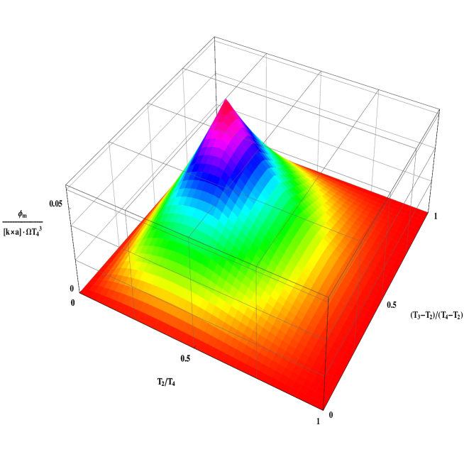
Figure 2: Dependence of the gyroscope phase on the position of the second and third pulse.

One can see that the phase (70) has only one maximum and that this maximum occurs for the double-loop interferometer shown in Fig. 1(a), when

$$s_{j}=1~{}\text{and~{}}t_{2}=1/4,t_{3}=3/4,$$ (71)

and $\phi_{m}$ is given by Eq. (7).

Nevertheless, one has to move out of the point (71) at least slightly to wash out contributions from the stimulated echo (62). Let us consider this case. If

$$s_{j}=1-\sigma_{j}$$ (72)

and $\sigma_{j}\ll 1,$ then from Eqs. (66) one finds with accuracy up to second order terms in $\sigma_{j},$ that the second and the third pulses have to be located at

$$t_{2} \approx\dfrac{1}{4}\left(1+\dfrac{9}{8}\sigma_{1}-\sigma_{2}-\dfrac{1}{8}\sigma_{4}+\dfrac{3}{4}\sigma_{1}\sigma_{2}-\dfrac{3}{16}\sigma_{1}\sigma_{4}+\dfrac{1}{4}\sigma_{2}\sigma_{4}+\dfrac{9}{32}\sigma_{1}^{2}-\sigma_{2}^{2}-\dfrac{3}{32}\sigma_{4}^{2}\right),$$ (73a)

$$t_{3} \approx\dfrac{1}{4}\left(3-\dfrac{3}{8}\sigma_{1}+\sigma_{2}-\dfrac{5}{8}\sigma_{4}+\dfrac{1}{4}\sigma_{2}\sigma_{4}-\dfrac{1}{16}\sigma_{1}\sigma_{4}-\dfrac{5}{4}\sigma_{1}\sigma_{2}+\dfrac{15}{32}\sigma_{1}^{2}+\sigma_{2}^{2}-\dfrac{13}{32}\sigma_{4}^{2}\right).$$ (73b)

We found these values from Eqs. (66a) and (66b). Substituting them into Eq. (66c) one gets the phase matching condition, in the first order over $\sigma_{j},$

$$\sigma_{4}-2\sigma_{3}+2\sigma_{2}-\sigma_{1}=0,$$ (74)

and the equality in the second order. We calculate, with the same accuracy, the main term (70) in the gyroscope phase,

$$\psi\approx\dfrac{1}{16}-\dfrac{1}{48}\sigma_{4}-\dfrac{1}{24}\sigma_{2}-\allowbreak\dfrac{45}{1024}\sigma_{1}^{2}-\dfrac{1}{16}\sigma_{2}^{2}-\dfrac{13}{1024}\sigma_{4}^{2}+\dfrac{3}{32}\sigma_{1}\sigma_{2}-\dfrac{3}{512}\sigma_{1}\sigma_{4}+\dfrac{1}{32}\sigma_{2}\sigma_{4},$$ (75)

while all terms in the zero-order over $\sigma_{j},$ calculated using Table 1 and the rule (69), are presented in Table 2. In the last two columns of this table and of Table 3 below we calculated phase for Cs interferometer ($m=2.21\times 10^{-22}~{}$g, $k=1.47\times 10^{5}~{}$cm${}^{\text{-1}}$) for $g_{z}=-980~{}cm/s^{2},$ $T_{4}=0.8~{}s,$ $R=6.72\times 10^{8}$ cm, latitude 41^∘.

Table 2: Atomic gyroscope phase shifts; column1, the general case; column 2, for the wave vector $\mathbf{k}$ and launch momentum $\mathbf{p}$ in the west-east and vertical directions; columns 3 and 4 represent the absolute and the relative phase shifts when $p=0$ for Cs gyroscope

$\begin{array}[c]{ccccccc}\vskip 3.0pt plus 1.0pt minus 1.0pt\dfrac{3\Omega^{2}}{32m}\left[\left(\mathbf{k}\boldsymbol{\nu}\right)\left(\mathbf{p}\boldsymbol{\nu}\right)-\left(\mathbf{kp}\right)\right]T_{4}^{3}&&0&&0&&0\\ \vskip 3.0pt plus 1.0pt minus 1.0pt\dfrac{1}{16}\boldsymbol{\Omega}\cdot\left(\mathbf{k}\times\mathbf{a}\right)T_{4}^{3}&&\begin{array}[c]{c}\vskip 3.0pt plus 1.0pt minus 1.0pt-\dfrac{1}{16}k\nu_{y}g_{z}\Omega T_{4}^{3}\\ -\dfrac{1}{16}k\nu_{y}\Omega^{3}RT_{4}^{3}\end{array}&&\begin{array}[c]{c}\vskip 3.0pt plus 1.0pt minus 1.0pt254\\ 0.92\end{array}&&\begin{array}[c]{c}\vskip 3.0pt plus 1.0pt minus 1.0pt1\\ 3.6\times 10^{-3}\end{array}\\ \vskip 3.0pt plus 1.0pt minus 1.0pt\dfrac{3\hbar}{64m}\left[\left(\mathbf{k}\cdot\boldsymbol{\nu}\right)^{2}-k^{2}\right]\Omega^{2}T_{4}^{3}&&-\dfrac{3\hbar k^{2}}{64m}\Omega^{2}T_{4}^{3}&&-1.32\times 10^{-5}&&-5.2\times 10^{-8}\\ \vskip 3.0pt plus 1.0pt minus 1.0pt-\dfrac{3}{64}\left[\left(\mathbf{k}\cdot\mathbf{a}\right)-\left(\mathbf{k}\cdot\boldsymbol{\nu}\right)\left(\mathbf{a}\cdot\boldsymbol{\nu}\right)\right]\Omega^{2}T_{4}^{4}&&0&&0&&0\\ \vskip 3.0pt plus 1.0pt minus 1.0pt-\dfrac{1}{16m}\left(\boldsymbol{\nu}\times\mathbf{k}\right)\cdot\mathbf{p}\Omega^{3}T_{4}^{4}&&\dfrac{\nu_{y}kp}{16m}\Omega^{3}T_{4}^{4}&&0&&0\\ \vskip 3.0pt plus 1.0pt minus 1.0pt-\dfrac{1}{64m}\mathbf{k}\cdot\mathbf{p}T_{4}^{3}T_{zz}&&0&&0&&0\\ \vskip 3.0pt plus 1.0pt minus 1.0pt-\dfrac{\hbar k^{2}}{128m}T_{4}^{3}T_{zz}&&-\dfrac{\hbar k^{2}}{128m}T_{4}^{3}T_{zz}&&-1.21\times 10^{-3}&&4.8\times 10^{-6}\\ \vskip 3.0pt plus 1.0pt minus 1.0pt-\dfrac{1}{128}\mathbf{k}\cdot\mathbf{a}T_{4}^{4}T_{zz}&&0&&0&&0\\ \vskip 3.0pt plus 1.0pt minus 1.0pt\dfrac{3}{64m}\left(\mathbf{n}\cdot\boldsymbol{\nu}\right)\left(\mathbf{k}\cdot\mathbf{n}\right)\left(\boldsymbol{\nu}\cdot\mathbf{p}\right)T_{4}^{3}T_{zz}&&0&&0&&0\\ \vskip 3.0pt plus 1.0pt minus 1.0pt\dfrac{3\hbar}{128m}\left(\mathbf{n}\cdot\boldsymbol{\nu}\right)\left(\mathbf{k}\cdot\mathbf{n}\right)\left(\boldsymbol{\nu}\cdot\mathbf{k}\right)T_{4}^{3}T_{zz}&&0&&0&&0\\ \vskip 3.0pt plus 1.0pt minus 1.0pt\dfrac{3}{128}\left(\mathbf{n}\cdot\boldsymbol{\nu}\right)\left(\mathbf{k}\cdot\mathbf{n}\right)\left(\boldsymbol{\nu}\cdot\mathbf{a}\right)T_{4}^{4}T_{zz}&&0&&0&&0\\ \vskip 3.0pt plus 1.0pt minus 1.0pt-\dfrac{3}{64m}\left(\mathbf{n}\cdot\boldsymbol{\nu}\right)\left[\boldsymbol{\nu}\cdot\left(\mathbf{n}\times\mathbf{k}\right)\right]\left(\boldsymbol{\nu}\cdot\mathbf{p}\right)\Omega T_{4}^{4}T_{zz}&&-\dfrac{3kp}{64m}\nu_{y}\nu_{z}^{2}\Omega T_{4}^{4}T_{zz}&&0&&0\\ \vskip 3.0pt plus 1.0pt minus 1.0pt-\dfrac{3\hbar}{128m}\left(\mathbf{n}\cdot\boldsymbol{\nu}\right)\left[\boldsymbol{\nu}\cdot\left(\mathbf{n}\times\mathbf{k}\right)\right]\left(\boldsymbol{\nu}\cdot\mathbf{k}\right)\Omega T_{4}^{4}T_{zz}&&0&&0&&0\\ \vskip 3.0pt plus 1.0pt minus 1.0pt\dfrac{3}{64m}\left[\left(\boldsymbol{\nu}\times\mathbf{n}\right)\cdot\left(\boldsymbol{\nu}\times\mathbf{p}\right)\right]\left(\mathbf{k}\cdot\mathbf{n}\right)T_{4}^{3}T_{zz}&&0&&0&&0\\ \vskip 3.0pt plus 1.0pt minus 1.0pt\dfrac{3\hbar}{128m}\left[\left(\boldsymbol{\nu}\times\mathbf{n}\right)\cdot\left(\boldsymbol{\nu}\times\mathbf{k}\right)\right]\left(\mathbf{k}\cdot\mathbf{n}\right)T_{4}^{3}T_{zz}&&0&&0&&0\\ \vskip 3.0pt plus 1.0pt minus 1.0pt-\dfrac{3}{64m}\left[\left(\boldsymbol{\nu}\times\mathbf{n}\right)\cdot\left(\boldsymbol{\nu}\times\mathbf{p}\right)\right]\left[\boldsymbol{\nu}\cdot\left(\mathbf{n}\times\mathbf{k}\right)\right]\Omega T_{4}^{4}T_{zz}&&-\dfrac{3kp\nu_{y}^{3}}{64m}\Omega T_{4}^{4}T_{zz}&&0&&0\\ \vskip 3.0pt plus 1.0pt minus 1.0pt-\dfrac{3\hbar}{128m}\left[\left(\boldsymbol{\nu}\times\mathbf{n}\right)\cdot\left(\boldsymbol{\nu}\times\mathbf{k}\right)\right]\left[\boldsymbol{\nu}\cdot\left(\mathbf{n}\times\mathbf{k}\right)\right]\Omega T_{4}^{4}T_{zz}&&0&&0&&0\\ \vskip 3.0pt plus 1.0pt minus 1.0pt\dfrac{3}{64m}\left[\left(\boldsymbol{\nu}\times\mathbf{n}\right)\cdot\mathbf{p}\right]\left(\mathbf{k}\cdot\mathbf{n}\right)\Omega T_{4}^{4}T_{zz}&&0&&0&&0\\ \vskip 3.0pt plus 1.0pt minus 1.0pt\dfrac{3\hbar}{128m}\left[\left(\boldsymbol{\nu}\times\mathbf{n}\right)\cdot\mathbf{k}\right]\left(\mathbf{k}\cdot\mathbf{n}\right)\Omega T_{4}^{4}T_{zz}&&0&&0&&0\\ \vskip 3.0pt plus 1.0pt minus 1.0pt\dfrac{3}{128}\left[\left(\boldsymbol{\nu}\times\mathbf{n}\right)\cdot\left(\boldsymbol{\nu}\times\mathbf{a}\right)\right]\left(\mathbf{k}\cdot\mathbf{n}\right)T_{4}^{4}T_{zz}&&0&&0&&0\end{array}$

VII.2 Atomic accelerometer

One can use the four-pulse interferometer to eliminate third-order contributions to the interferometer phase in order to increase the accuracy of acceleration measurements. In this case wave vectors and relative positions of the second and the third pulses have to satisfy Eqs. (64) for $n=0,~{}1,$ and $3.$ Resolving these equations with respect to wave vectors of the first, second, and third pulses and requiring that at least one of the pulse is comprised of counterpropagating waves, one finds

$$s_{1} =s_{4}\dfrac{\left(1-t_{3}\right)\left(1-t_{2}\right)\left(1+t_{2}+t_{3}\right)}{t_{2}t_{3}\left(t_{2}+t_{3}\right)},$$ (76a)

$$s_{2} =\dfrac{s_{4}}{2}\dfrac{1-t_{3}^{2}}{t_{2}\left(t_{3}^{2}-t_{2}^{2}\right)},$$ (76b)

$$s_{3} =\dfrac{s_{4}}{2}\dfrac{1-t_{2}^{2}}{t_{3}\left(t_{3}^{2}-t_{2}^{2}\right)},$$ (76c)

$$s_{4} =\min\left[\dfrac{t_{2}t_{3}\left(t_{2}+t_{3}\right)}{\left(1-t_{3}\right)\left(1-t_{2}\right)\left(1+t_{2}+t_{3}\right)},\dfrac{2t_{2}\left(t_{3}^{2}-t_{2}^{2}\right)}{1-t_{3}^{2}},\dfrac{2t_{3}\left(t_{3}^{2}-t_{2}^{2}\right)}{1-t_{2}^{2}},1\right].$$ (76d)

To get the main contribution to the interferometer phase one should perform the replacement (69) for $n=2$ in the very first cell of Table 1. It yields the following expression:

$$\phi_{m}=-\dfrac{s_{4}\left(1-t_{3}\right)\left(1-t_{2}\right)}{\allowbreak 2\left(t_{2}+t_{3}\right)}\mathbf{k}\cdot\mathbf{a}T_{4}^{2}.$$ (77)

This dependence is shown in Fig. 3.

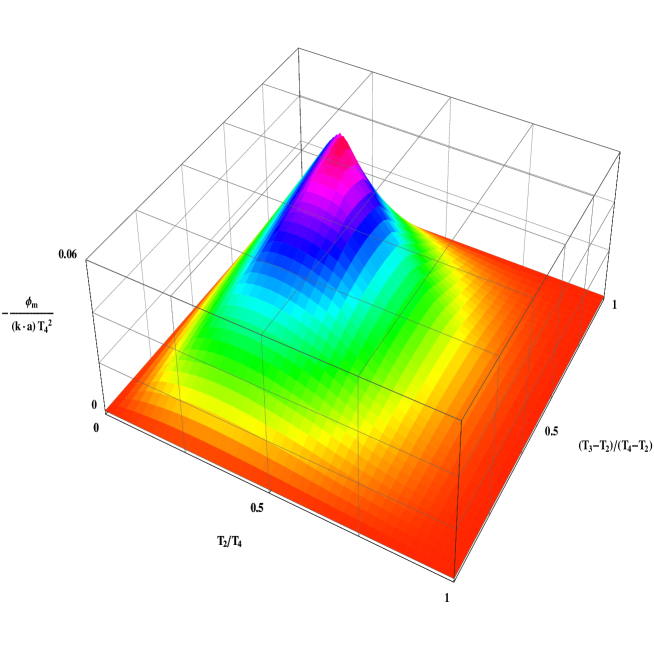
Figure 3: The same as in Fig. 2, but for the phase of accelerometer.

One sees that only one maximum of the accelerometer’s phase corresponds to values of $t_{2}$ and $t_{3}$ given by Eq. (9). Substituting these values into Eqs. (76) one verifies that the maximum of accelerometer phase occurs when all pulses are comprised of counterpropagating fields, $s_{j}=1.$

From Eq. (9) one can see that $T_{4}-T_{3}\not=T_{2}$ and therefore the contribution from stimulated echo processes given by Eq. (62) is washed out after averaging over momenta.

Different terms in the accelerometer phase can be obtained from Table 1 using the replacement (69). They are presented in Table 3.

Table 3: The same as in Table 1, but for the four-pulse interferometer shown in Fig. 1(c). The last two columns are for the phase shifts’ numerical and relative values of the Cs interferometer for ${}p=0$.

$\begin{array}[c]{ccccc}\vskip 3.0pt plus 1.0pt minus 1.0pt-\dfrac{\sqrt{5}-2}{4}\mathbf{k}\cdot\mathbf{a}T_{4}^{2}&\begin{array}[c]{c}\vskip 3.0pt plus 1.0pt minus 1.0pt-\dfrac{\sqrt{5}-2}{4}kg_{z}T_{4}^{2}\\ -\dfrac{\sqrt{5}-2}{4}k\Omega_{y}^{2}RT_{4}^{2}\end{array}&&\begin{array}[c]{c}\vskip 3.0pt plus 1.0pt minus 1.0pt5.46\times 10^{6}\\ -1.13\times 10^{4}\end{array}&\begin{array}[c]{c}1\\ 2.0\times 10^{-3}\end{array}\\ \vskip 3.0pt plus 1.0pt minus 1.0pt-\dfrac{\sqrt{5}-2}{2m}\left(\boldsymbol{\Omega}\times\mathbf{k}\right)\cdot\mathbf{p}T_{4}^{2}&0&&0&0\\ \vskip 3.0pt plus 1.0pt minus 1.0pt-\dfrac{8-3\sqrt{5}}{64}\left[\left(\mathbf{k}\cdot\mathbf{a}\right)-\left(\mathbf{k}\cdot\boldsymbol{\nu}\right)\left(\mathbf{a}\cdot\boldsymbol{\nu}\right)\right]\Omega^{2}T_{4}^{4}&\begin{array}[c]{c}\vskip 3.0pt plus 1.0pt minus 1.0pt-\dfrac{8-3\sqrt{5}}{64}kg_{z}\Omega_{y}^{2}T_{4}^{4}\\ -\dfrac{8-3\sqrt{5}}{64}k\Omega^{2}\Omega_{y}^{2}RT_{4}^{4}\end{array}&&\begin{array}[c]{c}\vskip 3.0pt plus 1.0pt minus 1.0pt3.60\times 10^{-3}\\ 1.31\times 10^{-5}\end{array}&\begin{array}[c]{c}6.6\times 10^{-10}\\ 2.4\times 10^{-12}\end{array}\\ \vskip 3.0pt plus 1.0pt minus 1.0pt-\dfrac{8-3\sqrt{5}}{48m}\left(\boldsymbol{\nu}\times\mathbf{k}\right)\cdot\mathbf{p}\Omega^{3}T_{4}^{4}&0&&&\\ \vskip 3.0pt plus 1.0pt minus 1.0pt-\dfrac{8-3\sqrt{5}}{384}\mathbf{k}\cdot\mathbf{a}T_{4}^{4}T_{zz}&\begin{array}[c]{c}\vskip 3.0pt plus 1.0pt minus 1.0pt\underline{-\dfrac{8-3\sqrt{5}}{384}kg_{z}T_{3}^{4}T_{zz}}\\ \underleftarrow{-\dfrac{8-3\sqrt{5}}{384}k\Omega_{y}^{2}RT_{4}^{4}T_{zz}}\end{array}&\begin{array}[c]{c}\dfrac{8-3\sqrt{5}}{192}kg_{z}T_{4}^{4}T_{zz}\\ \dfrac{8-3\sqrt{5}}{192}k\Omega_{y}^{2}RT_{4}^{4}T_{zz}\end{array}&\begin{array}[c]{c}\vskip 3.0pt plus 1.0pt minus 1.0pt-1.16\\ 2.40\times 10^{-3}\end{array}&\begin{array}[c]{c}2.1\times 10^{-7}\\ 4.4\times 10^{-10}\end{array}\\ \vskip 3.0pt plus 1.0pt minus 1.0pt\dfrac{8-3\sqrt{5}}{128}\left(\mathbf{n}\cdot\boldsymbol{\nu}\right)\left(\mathbf{k}\cdot\mathbf{n}\right)\left(\boldsymbol{\nu}\cdot\mathbf{a}\right)T_{4}^{4}T_{zz}&\underline{\dfrac{8-3\sqrt{5}}{128}\nu_{z}^{2}kg_{z}T_{3}^{4}T_{zz}}&&&\\ \vskip 3.0pt plus 1.0pt minus 1.0pt-\dfrac{8-3\sqrt{5}}{64m}\left(\mathbf{n}\cdot\boldsymbol{\nu}\right)\left[\boldsymbol{\nu}\cdot\left(\mathbf{n}\times\mathbf{k}\right)\right]\left(\boldsymbol{\nu}\cdot\mathbf{p}\right)\Omega T_{4}^{4}T_{zz}&0&&&\\ \vskip 3.0pt plus 1.0pt minus 1.0pt-\dfrac{8-3\sqrt{5}\hbar}{128m}\left(\mathbf{n}\cdot\boldsymbol{\nu}\right)\left[\boldsymbol{\nu}\cdot\left(\mathbf{n}\times\mathbf{k}\right)\right]\left(\boldsymbol{\nu}\cdot\mathbf{k}\right)\Omega T_{4}^{4}T_{zz}&0&&&\\ \vskip 3.0pt plus 1.0pt minus 1.0pt-\dfrac{8-3\sqrt{5}}{64m}\left[\left(\boldsymbol{\nu}\times\mathbf{n}\right)\cdot\left(\boldsymbol{\nu}\times\mathbf{p}\right)\right]\left[\boldsymbol{\nu}\cdot\left(\mathbf{n}\times\mathbf{k}\right)\right]\Omega T_{4}^{4}T_{zz}&0&&&\\ \vskip 3.0pt plus 1.0pt minus 1.0pt-\dfrac{\left(8-3\sqrt{5}\right)\hbar}{128m}\left[\left(\boldsymbol{\nu}\times\mathbf{n}\right)\cdot\left(\boldsymbol{\nu}\times\mathbf{k}\right)\right]\left[\boldsymbol{\nu}\cdot\left(\mathbf{n}\times\mathbf{k}\right)\right]\Omega T_{4}^{4}T_{zz}&0&&&\\ \vskip 3.0pt plus 1.0pt minus 1.0pt\dfrac{8-3\sqrt{5}}{64m}\left[\left(\boldsymbol{\nu}\times\mathbf{n}\right)\cdot\mathbf{p}\right]\left(\mathbf{k}\cdot\mathbf{n}\right)\Omega T_{4}^{4}T_{zz}&0&&&\\ \vskip 3.0pt plus 1.0pt minus 1.0pt\dfrac{\left(8-3\sqrt{5}\right)\hbar}{128m}\left[\left(\boldsymbol{\nu}\times\mathbf{n}\right)\cdot\mathbf{k}\right]\left(\mathbf{k}\cdot\mathbf{n}\right)\Omega T_{4}^{4}T_{zz}&0&&&\\ \vskip 3.0pt plus 1.0pt minus 1.0pt\dfrac{8-3\sqrt{5}}{128}\left[\left(\boldsymbol{\nu}\times\mathbf{n}\right)\cdot\left(\boldsymbol{\nu}\times\mathbf{a}\right)\right]\left(\mathbf{k}\cdot\mathbf{n}\right)T_{4}^{4}T_{zz}&\begin{array}[c]{c}\vskip 3.0pt plus 1.0pt minus 1.0pt\underline{\dfrac{8-3\sqrt{5}}{128}k\nu_{y}^{2}g_{z}T_{3}^{4}T_{zz}}\\ \underleftarrow{\dfrac{8-3\sqrt{5}}{128}k\nu_{y}^{2}\Omega^{2}RT_{4}^{4}T_{zz}}\end{array}&&&\end{array}$

VIII Discussion

In this paper we showed that, in the presence of inertial forces and homogeneous acceleration gradient, the density matrix in the Wigner representation in the free space still obeys classical Liouville equation for the distribution function. It allows us to get interferometers’ phases without calculating path integrals.

For all interferometers under consideration we calculate phase shifts up to terms proportional to $T^{4}$ for an arbitrary constant in time acceleration and rotation.

Using double-loop interferometers $\pi/2-\pi-\pi-\pi/2$ one can eliminate the phase dependence on the acceleration only and get an interferometer with the main phase term proportional to the cross product of acceleration and rotation frequency. One can use this interferometer as a gyroscope to measure rotation frequency components perpendicular to the acceleration. Even for the rotation frequency as small as the Earth rotation rate, the phase of this gyroscope can achieve $\phi_{m}\sim 100.$ Eliminating the acceleration term, which is typically five orders of magnitude larger, could be incomplete if pulse areas are not precisely equal to $\pi/2$ or $\pi,$ because in this case stimulated echo processes, which are extremely sensitive to the acceleration, contribute to the probability of the particles’ excitation. To exclude these processes we propose to drive Raman transitions between hyperfine atomic sublevels by a pulse of travelling noncounterpropagating optical waves. For this goal one can use even slightly noncounterpropagating fields having effective wave vectors given by Eqs. (65) and (72), where the small parameter $\sigma_{j}$ determines the deviation of the pulse $j$ wave vector from the maximum value $k.$ If wave vectors satisfy the phase matching condition (1a) for double-loop interferometer but violate the phase-matching condition (1b) for stimulated echo, i.e., if

$$\sigma_{dl} =\sigma_{4}-2\sigma_{3}+2\sigma_{2}-\sigma_{1}=0,$$ (78a)

$$\sigma_{st} =\sigma_{4}-\sigma_{3}-\sigma_{2}+\sigma_{1}\not=0,$$ (78b)

integrands in Eq. (62) for probabilities of excitation associated with stimulated echo processes become rapidly oscillating in space function, which have the period of the order of$\ \lambda/\sigma_{st},$ where $\lambda=2\pi/k$ is the effective wavelength. When

$$\dfrac{\lambda}{s_{cloud}}\ll\sigma_{st}\ll 1,$$ (79)

where $s_{cloud}$ is the initial atomic cloud size, in the case when the initial atom density is smooth in space, probabilities (62) become exponentially small with respect to the parameter $\sigma_{st}s_{cloud}/\lambda\gg 1.$ In addition to arguments related to the difference in phase matching conditions, one can expect further decrease of probabilities (62) due to the fact that pulses are not properly positioned in time [$1-t_{3}\not=t2,$ where $t_{j}$ are given by Eqs. (73)] to produce the stimulated echo. We obtained the required pulses’ positions and the main term in the gyroscope phase for arbitrary $\sigma_{j},$ see Eqs. (73), (70a), and (75). But it is sufficient for only two effective wave vectors to have $\sigma_{j}\not=0.$ If, for example,

$$\sigma_{3}=\sigma_{4}=0~{}\text{and }\sigma_{2}=\dfrac{\sigma_{1}}{2}\not=0,$$ (80)

then $\sigma_{st}=\dfrac{\sigma_{1}}{2},$ second and third pulses have to be applied at moments

$$T_{2} \approx\dfrac{T_{4}}{4}\left(1+\dfrac{5}{8}\sigma_{1}+\dfrac{13}{32}\sigma_{1}^{2}\right),$$ (81a)

$$T_{3} \approx\dfrac{3}{4}T_{4}\left(1+\dfrac{1}{24}\sigma_{1}+\dfrac{1}{32}\sigma_{1}^{2}\right)$$ (81b)

and gyroscope phase is given by

$$\phi_{m}=\dfrac{1}{16}\left(1-\dfrac{1}{3}\sigma_{1}-\dfrac{13}{64}\sigma_{1}^{2}\right)\left(\mathbf{k}\times\mathbf{a}\right)\cdot\mathbf{\Omega}T_{4}^{3}.$$ (82)

A “side-effect” of using Raman pulses with nonequal effective wave vectors is that in this case one gets Ramsey fringes, i.e., excitation probability oscillating dependences on the Raman detuning $\delta_{12}$ having period of the order of the inverse time delay between pulses $T^{-1}$ [see Ramsey phases $\phi_{R}$ (54c) and (60d) for single- and double-loop interferometers]. Evidently, this new type of Ramsey fringes arises because even for Raman pulses with copropagating effective wave vectors, in the condition of the Doppler phase cancellation, time separations between pulses $T_{j}$ enter with weight factors $\mathbf{k}_{j},$ while these factors are absent in expressions for the Ramsey phase. In contrast to the previously proposed c20 and observed c6 Raman-Ramsey fringes on Doppler broadened two-quantum transitions based on the use of Raman pulses having counterpropagating effective wave vectors, Ramsey fringes found here do not undergo recoil splitting, i.e., they are centered at the two-quantum line center.

Double-loop interferometer shown in Fig. 1(c) allows one to get the phase where all cubic in $T$ terms are eliminated and can serve as an accelerometer. We expect that owing to this cancellation, the accuracy of the acceleration measurement can be increased.

Thus in this paper we propose the following scenario for the atomic gravity and rotation sensing. First one measures acceleration $\mathbf{a}$ using three mutually perpendicular double-loop accelerometers. Afterwards, one uses the spatial-domain atomic gyroscope c4 , orients it in the plane perpendicular to $\mathbf{a}$ and measures the component of the rotation frequency $\boldsymbol{\mathbf{\Omega}}$ along $\mathbf{a}.$ Then one uses two mutually perpendicular time-domain double-loop gyroscopes to get components of $\boldsymbol{\mathbf{\Omega}}$ perpendicular to $\mathbf{a.}$

Further obvious step here could be the consideration of multiple-loop interferometers. In general for an interferometer consisting of $\ell$ unidirectional pulses (first and last are $\pi/2$ pulses, others are $\pi$ pulses), having the same wave vector, one has $\ell-2$ parameters $t_{j}=T_{j}/T_{\ell}$ $\left(j=2,~{}\ldots,~{}\ell-1\right)$, which can be chosen as a root of the system of $\ell-2$ equations

$$1-2t_{\ell-1}^{u_{j}}+2t_{\ell-2}^{u_{j}}+\ldots+\left(-1\right)^{\ell}2t_{2}^{u_{j}}=0$$ (83)

to eliminate phase terms evolving as $T_{\ell}^{u_{1}},$ …,$T_{\ell}^{u_{\ell-2}}.$ In the array $\mathbf{u}=\left(u_{1},\ldots,u_{\ell-2}\right)$ one of parameters $u_{j}$ has to be equal to 1, to eliminate the Doppler phase, while the choice of other parameters depends on phenomena one would like to sense using the interferometer. Remaining noneliminated phase terms evolving as $T_{\ell}^{v}$ can be obtained from Table 1 by replacement of

$$T_{3}^{v}\rightarrow\dfrac{1-2t_{\ell-1}^{v}+2t_{\ell-2}^{v}+\ldots+\left(-1\right)^{\ell}2t_{2}^{v}}{1-2^{1-v}}T_{\ell}^{v}.$$ (84)

The case of four-pulse interferometers is considered above in detail. Using five-pulse interferometers one can eliminate $T_{5}^{4}$ dependencies. For gyroscope $\mathbf{u}=\left(1,2,4\right),$ we found the numeric solution of system (83),

$$t_{2}=0.16615,~{}t_{3}=0.54057,~{}t_{4}=0.87442.$$ (85)

This gyroscope phase is given by

$$\phi_{m}=-1.0143\times 10^{-2}\boldsymbol{\mathbf{\Omega}}\cdot\left(\mathbf{k}\times\mathbf{a}\right)T_{5}^{3}+O\left(T_{5}^{5}\right).$$ (86)

For the Cs gyroscope with the same parameters as in Table 2, $\phi_{m}\approx-41.2.$

For the five-pulse accelerometer, $\mathbf{u}=\left(1,3,4\right),$ one finds

$$t_{2}=0.20594,~{}t_{3}=0.594\,37,~{}t_{4}=0.88843,$$ (87)

and the phase is given by

$$\phi_{m}=2.1557\times 10^{-2}\mathbf{k}\cdot\mathbf{a}T_{5}^{2}+O\left(T_{5}^{5}\right).$$ (88)

For the Cs accelerometer with the same parameters as in Table 3, $\phi_{m}\approx-2.00\times 10^{6}.$

Another example of five-pulse interferometer is a “figure 8 1/2” interferometer proposed in c121 to eliminate $T_{5}^{2}$ and $T_{5}^{3}$ terms, such as the dominate contribution to the phase is caused by the influence of space-time curvature.

Consider also six-pulse interferometer. One can use this pulse sequence to eliminate all phase terms arising as a result of the atom motion to the accuracy $T_{6}^{4}$ choosing $\mathbf{u}=\left(1,2,3,4\right).$ The numerical solution of the system (83) is given by

$$t_{2}=9.5492\times 10^{-2},~{}t_{3}=0.34549,~{}t_{4}=0.65451,~{}t_{5}=0.90451.$$ (89)

Of course, one cannot use this interferometer to sense atomic motion. But one can use it for the precise measurement of the other spectroscopic data. The accuracy of this measurement improves when the time of evolution $T_{6}$ increases. Earth gravity and rotation superimpose limitation on this time. This time can be increased in the microgravity environment. We actually propose to use the six-pulse interferometer instead of transferring experiments into microgravity environment.

Possible examples here are measurement of levels polarizability c21 or observation of the Aharonov-Bohm effect c22 . We also believe that one can insert additional $\pi$ pulses in the scheme of the recoil frequency measurement c6 to make this measurement independent on the gravity, gravity gradient and the Earth rotation.

Recoil diagrams for five- and six-pulse interferometers are shown in Fig. 4.

Figure 4: Recoil diagrams for the five-pulse gyroscope (a), accelerometer (b) and six-pulse interferometer insensitive to both rotation and acceleration.

Regarding the six-pulse interferometer, one sees that it has to be protected from two kinds of the stimulated echo processes produced by the sequences of pulses $\left\{1,2,5,6\right\}$ and $\left\{1,3,4,6\right\}.$ A similar note can be made regarding the “figure 8 1/2” interferometer c121 , where both stimulated echo produced by pulses $\left\{1,2,4,5\right\}$ and one-loop interferometer produced by pulses $\left\{1,3,5\right\}$ have to be excluded. An effective technique of eliminating all these unwanted signals is using Raman pulses with nonequal effective wave vectors, as we demonstrated and analyzed above for the double-loop atomic gyroscope.

References

• (1) B. Dubetsky, A. P. Kazantsev, V. P. Chebotayev, and V. P. Yakovlev, Pisโ€™ma Zh. Eksp. Teor. Fiz. 39, 531 (1984) [JETP Lett. 39, 649 (1985)].
• (2) J. F. Clauser, in Proceedings of the International Workshop on Matter Wave Interferometry in the Light of Schrรถdingerโ€™s Wave Mechanics, edited by G. Badirek, H. Rauch, and A. Zeilinger,1987, Physica B & C 151, 262 (1988).
• (3) M. Kasevich and S. Chu, Phys. Rev. Lett., 67, 181 (1991).
• (4) T. L. Gustavson, A. Landragin, and M. A. Kasevich, Class. Quantum. Grav. 17, 2385 (2000); T. L. Gustavson, P. Bouyer, and M. A. Kasevich, Phys. Rev. Lett. 78, 2046 (1997).
• (5) M. J. Snadden, J. M. McGuirk, P. Bouyer, K. G. Haritos, and M. A. Kasevich, Phys. Rev. Lett. 81, 971 (1998); J. M. McGuirk, G. T. Foster, J. B. Fixler, M. J. Snadden, and M. A. Kasevich, Phys. Rev. A 65, 033608 (2002).
• (6) D. S. Weiss, B. C. Young, and S. Chu, Phys. Rev. Lett. 70, 2706 (1993); D. S. Weiss, B. C. Young, and S. Chu, Appl. Phys. B 59, 217 (1994).
• (7) A. Peters, C. Keng Yeow, and S. Chu, Nature 400, 849 (1999); A. Peters, K. Y. Chung, and S. Chu, Metrologia 38, 25 (2001).
• (8) J. Audretsch and K.-P. Marzlin, Phys. Rev. A 50, 2080, (1994).
• (9) J. Audretsch and K.-P. Marzlin, J. Phys. II 4, 2073 (1994).
• (10) K. Bongs, R. Launay, and M. A. Kasevich, http://arxiv.org/abs/quant-ph/0204102
• (11) Ch. J. Borde, C. R. Acad. Sci., Sรฉrie IV: Phys., Astrophys. 2, p. 509โ€“530 (2001); Ch. Antoine and Ch. J. Borde, J. Opt. B: Quantum Semiclassical Opt. 5 S199 (2003).
• (12) A. P. Kolโ€™chenko, S. G. Rautian, and R. I. Sokolovskii, Zh. Eksp. Teor. Fiz. 55, 1864 (1968) [Sov. Phys. JETP 28, 986 (1969)].
• (13) B. Dubetsky and P. R. Berman, Phys. Rev. A 56, R1091 (1997).
• (14) K.-P. Marzlin and J. Audretsch, Phys. Rev. A 53, 312 (1996).
• (15) J. M. McGuirk, G. T. Foster, J. B. Fixler, M. J. Snadden, and M. A. Kasevich, Phys. Rev. A 65, 033608 (2002).
• (16) A. Kumarakrishnan, S. B. Cahn, U. Shim, and T. Sleator, Phys. Rev. A 58, R3387 (1998).
• (17) B. Dubetsky and P. R. Berman, Phys. Rev. A 59, 2269 (1999).
• (18) B. Dubetsky and P. R. Berman, in Atom Interferometry, edited by P. R. Berman (Academic, Cambridge, MA, 1997), pp. 407-468, http://xxx.lanl.gov/abs/physics/0005078
• (19) P. Storey and C. Cohen-Tannoudji, J. Phys. II 4, 1999, (1994).
• (20) Density matrix in the Wigner representation could have negative sum of the diagonal matrix elements, $F\left(\mathbf{r,p,}t\right)\equiv Tr\left[\rho\left(\mathbf{r,p,}t\right)\right].$ Moreover, from Eqs. (52) and (59) and corresponding expressions for $\rho_{gg}\left(\mathbf{r,p,}t\right),$ one concludes that even in the absence of the forces, for the large recoil momentum, $\hbar k_{1}\gg\Delta p,$ $F\left(\mathbf{r,p,}t\right)$ can be negative in the vicinities of the points $\mathbf{p=}\pm\hbar\mathbf{k}_{1}/2.$ This circumstance should not create any difficulty in the interpretation, because it is impossible to introduce distribution function over positions and momenta for the gas of atoms with quantized center-of-mass degrees of freedom, and function $F\left(\mathbf{r,p,}t\right)$ does not have the meaning of this distribution function.
• (21) B. Young, M. Kasevich, and S. Chu, in Atom Interferometry, edited by P. R. Berman (Academic, Cambridge, MA, 1997), pp. 363-406.
• (22) N. F. Ramsey, Phys. Rev. 76, 996 (1949).
• (23) A. N. Oraevsky, IEEE Trans. Instrum. Meas. 17, 346 (1968).
• (24) V. S. Letokhov and B. D. Pavlik, Opt. Spektrosk, 32, 856 (1972).
• (25) V. P. Chebotaev and B. Ya. Dubetsky, Appl. Phys. 18, 217 (1979).
• (26) C. R. Ekstrom, J. Schmiedmayer, M. S. Chapman, T. D. Hammond, and D. E. Pritchard, Phys. Rev. A 51, 3883 (1995).
• (27) G. van der Zouw, M. Weber, J. Felber, R. Gรคhler, P. Geltenbort, and A. Zeilinger, Nucl. Instrum. Methods Phys. Res. A 440, 568 (2000).