The multiscale nature of streamers

Abstract

Streamers are a generic mode of electric breakdown of large gas volumes. They play a role in the initial stages of sparks and lightning, in technical corona reactors and in high altitude sprite discharges above thunderclouds. Streamers are characterized by a self-generated field enhancement at the head of the growing discharge channel. We briefly review recent streamer experiments and sprite observations. Then we sketch our recent work on computations of growing and branching streamers, we discuss concepts and solutions of analytical model reductions, we review different branching concepts and outline a hierarchy of model reductions.

1 Introduction

Streamer discharges are a fundamental physical phenomenon with many technical applications [1, 2, 3]. While their role in lightning waits for further studies [4, 5], new lightning related phenomena above thunderclouds have been discovered in the past 15 years to which streamer concepts can be directly applied [6, 7, 8, 9].

In past years, appropriate methods have become available to study and analyze these phenomena. Methods include plasma diagnostic methods, large scale computations as well as analysis of nonlinear fronts and moving boundaries. The aim of the present article is to briefly summarize progress in these different disciplines, to explain the mutual benefit and to give a glimpse on future research questions.

The overall challenge in the field is to understand the growth of single streamers as well as the conditions of branching or extinction and their interactions which would allow us to predict the overall multi-channel structure formed by a given power supply in a given gas. We remark that so-called dielectric breakdown models [10, 11] have been suggested to address this question, but they incorporate the underlying mechanisms on smaller scales in a too qualitative way.

Many of our arguments are qualitative as well, but in a different sense. The main theoretical interest of the present paper is in basic conservation laws, in the wide range of length and time scales that characterize a streamer, in physical mechanisms for instabilities, and in the question whether a given problem should be modelled in a continuous or a discrete manner. Answering these questions provides the basis for future quantitative predictions.

The paper is organized as follows: In Section 2 a short overview over current experimental questions, methods and results is given, and applications are briefly discussed. Sprite discharges above thunderclouds are reviewed. In Section 3, the microscopic mechanisms and modelling issues are discussed and characteristic scales are identified by dimensional analysis. In Section 4 numerical solutions for negative streamers in non-attaching gases are presented, the multiple scales of the process are discussed and a short view on numerical adaptive grid refinement is given. Section 5 summarizes an analytical model reduction to a moving boundary problem, sketches issues of charge conservation and transport and confronts two different concepts of streamer branching. Conclusion and summary can be found in Section 6.

2 Streamers and sprites, experiments, applications and observations

The emergence and propagation of streamers has a long research history. The basics of a theory of spark breakdown were developed in the 1930’ies by Raether, Loeb and Meek [12, 13].

2.1 Time resolved streamer measurements

The first experiments on streamers were carried out by Raether who took pictures of the development of a streamer in a cloud chamber [12]. In this experiment a discharge was generated by a short voltage pulse. The ions within the streamer region act as nuclei for water droplets that form in the cloud chamber. Photographs of these droplets show the shape of the avalanche or the emerging streamer.

Later the use of streak photography together with image intensifiers enabled researchers to take time resolved pictures of streamers [14, 15, 16]. Streak photographs show the evolution of a slit-formed section of the total picture as a function of time. Examples of streak photographies can be found in this volume [5].

Recently, ICCD (Intensified Charge Coupled Device) pictures yield very high temporal resolution, and at the same time a full picture of the discharge, rather than the one-dimensional subsection obtained with streak photography. First measurements since 1994 with 30 ns [17] and 5 ns [18] resolution showed the principle. Since 2001, a resolution of about 1 ns has been reached [19, 20, 21, 22, 23, 24]. Meanwhile, even shorter gate times are possible [25]. However, the C-B transition of the second positive system of N₂ is the most intensive and dominates the picture, and its lifetime is of the order of 1 to 2 ns at atmospheric pressure. Therefore, a further improvement of the temporal resolution of the camera does not improve the temporal resolution of the picture, but has to be payed with a lower spatial resolution and a lower photon number density. Our measurements with resolution down to about 1 ns therefore resolve the short time structure of streamers at atmospheric pressure down to the physical limit. Fig. 1 shows snapshots of positive streamers in ambient air emerging from a positive point electrode at the upper left corner of the picture and extending to a plane electrode at the lower end of the picture. The distance between point and plane is 4 cm and the applied voltage about 28 kV. The optics resolves all streamers within the 3D discharge, also within the depth. The filamentary structure of the streamers as well as their frequent branching is clearly seen on the left most picture with 300 ns exposure time. The rightmost picture has the shortest exposure time of 1 ns. It shows not the complete streamers, but only the actively growing heads of the channels where field and impact ionization rates are high. As a consequence, the other pictures have to be interpreted not as glowing channels, but as the trace of the streamer head within the exposure time. Streamer velocities can therefore directly be determined as trace length devided by exposure time.

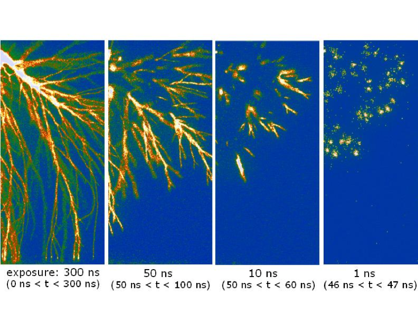
Figure 1: ICCD photographs in the present Eindhoven experiments of positive streamers in ambient air between point electrode in the upper left corner and plane electrode below. Only the right halves of the figures are shown. The gap spacing is 4 cm, the applied voltage is 28 kV. The exposure times of the photographs is 300, 50, 10 and $\sim$1 ns, the actual time intervals are given in brackets where $t=0$ is the approximate time when the streamers emerge from the upper point.

Most experimental work has been carried out on positive streamers in air [20, 24, 25, 26]. We wish to draw the reader’s attention to the work by Yi and Williams [23], who investigated the propagation of both anode and cathode-directed streamers, in almost pure N₂ and in N₂/O₂ mixtures. We will briefly interprete their results in Section 3.

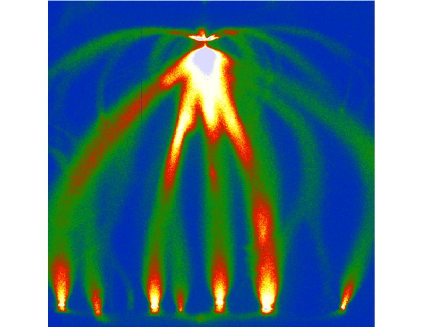
Figure 2: ICCD photograph of a positive streamer in ambient air in the same electrode configuration as in Fig. 1, but now powered with a transmission line transformer and a peak voltage of 60 kV [27]. The voltage pulse lasts about $\sim 100$ ns and limits the duration of the discharge; the exposure time of 20 $\mu$s accounts for the jitter of the voltage switching.

The experimental results depend not only on applied voltage, but also on further features of the external power supply. A glimpse is given in Fig. 2. For a further discussion of this feature, we refer to [24, 25, 26] and future analysis. Furthermore the results depend on the gas pressure [24] as will be further discussed below.

2.2 Applications

There are numerous applications of streamers in corona discharges [1]. Dust precipitators use DC corona to charge small particles and draw them out of a gas stream. This process is used in industry for already more than a century. Another wide spread application is charging photoconductors in copiers and laser printers. The first use of a pulsed discharge has been the production of ozone with a barrier configuration in 1854. This method is still being used [1] but pulsed corona discharges obtain the same ozone yield [28].

In the 1980’s the chemical activity of pulsed corona was recognized and investigated for the combined removal of SO₂, NO_x and fly ash [29, 30]. In the same period also the first experiments on water cleaning by pulsed corona were performed [31]. More results on combined SO₂/NO_x removal can be found in [1], recent results on degradation of phenol in water are given in [28] and [32]. More recently, the chemical reactivity is further explored for example in odor removal [33], tar removal from biogas [34] and killing of bacteria in water [35].

A new field is the combination of chemical and hydrodynamic effects. This can be used in plasma-assisted combustion [36] and flame control [37]. Purely electrohydrodynamic forces are studied in applications such as aerodynamic flow acceleration [3, 38] for aviation and plasma-assisted mixing [39].

Basically, these applications are based on at least one of three principles: 1) the deposition of streamer charge in the medium, 2) molecular excitations in the streamer head that initiate chemical processes, and 3) the coupling of moving space charge regions to gas convection [3]. The chemical applications are based on the exotic properties of the plasma in the streamer head that acts as a self-organized reactor: a space charge wave carries a confined amount of high energetic electrons that effectively ionize and excite the gas molecules. It is this active region that is seen in ICCD pictures like Fig. 1.

2.3 Sprite discharges above thunderclouds

Streamers can also be observed in nature. They play a role in creating the paths of sparks and lightning [4, 5, 40], and sensitive cameras showed the existence of so-called sprites [6, 41, 42] and blue jets [8, 43, 44] in the higher regions of the atmosphere above thunderclouds. With luck and experience, sprites can also be seen with naked eye. A scheme of sprites, jets and elves as the most frequently observed lightning related transious luminous events above lightning clouds is given in Fig. 3a.

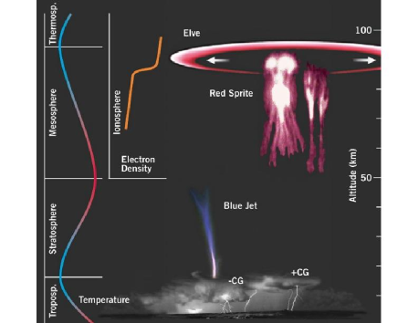
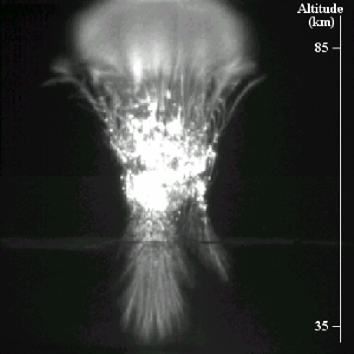
Figure 3: a) Scheme of transient luminous events above thunderclouds [45]. b) Photograph of a sprite. The altitude is indicated on the right. Courtesy of H.C. Stenbaek-Nielsen, Dept. Geophys., Univ. Fairbanks, Alaska.

Sprites have been observed between about 40 and 90 km height in the atmosphere. Above about 90 km, solar radiation maintains a plasma region, the so-called ionosphere. In this region, so-called elves can occur which are expanding rings created by electromagnetic resonances in the ionospheric plasma. Sprites, on the other hand, require a lowly or non-ionized medium, they can propagate from the ionosphere downwards or from some lower base upwards, or they can emerge at some immediate height and propagate upwards and downwards like in the event shown in Fig. 3b. A variety of sprite forms have been reported [7, 46]. The propagation direction and approximate velocity – their speed can exceed 10⁷ m/s [47] –, is known since researchers succeeded in taking movies [9]. A sequence of movie pictures can be found in this volume [5]. Telescopic images of sprites show that they are composed of a multitude of streamers (see Fig. 4). Blue jets propagate upwards from the top of thunderclouds, at speeds that are typically two orders of magnitude lower than those of sprites, and they have a characteristic conical shape and appear in a blueish color [43, 44]. Sprite discharges are the most frequent of these phenomena.

The approximate similarity relations between streamers and sprites are discussed in the next section. Sprites could therefore have similar physical and chemical effects as those discussed for streamer applications in the previous section. In fact, charge deposition in the medium and molecular excitations with subsequent chemical processes can be expected as well. On the other hand, we will show below by dimensional analysis that generation of gas convection is unlikely in sprites.

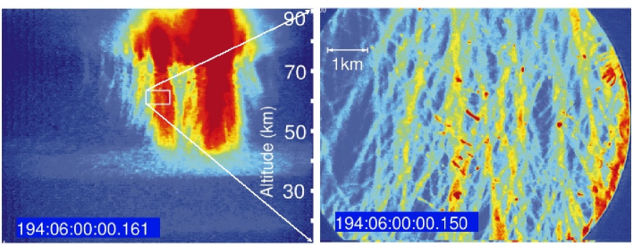
Figure 4: Telescopic image of a sprite discharge. The right photograph zooms into the white rectangle of the left photograph. These pictures are taken from [7].

3 Microscopic modelling

3.1 An overview of modelling aspects

The basic microscopic ingredients for a streamer discharge are
1) the generation of electrons and ions in regions of high electric field,
2) drift and diffusion of the electrons in the local field, and
3) the modification of the externally applied field by the generated space charges.
While avalanches evolve in a given background field, streamers have a characteristic nonlinear coupling between densities and fields: The space charges change the field, and the field determines the drift and reaction rates. More specifically, the streamer creates a self-consistent field enhancement at its tip which allows it to penetrate into regions where the background field is too low for an efficient ionization reaction to take place. In this sense, streamers are similar to mechanical fractures in solid media: either the electric or the mechanical forces focus at the tips of the extending structures.

While these general features are the same, models vary in the following aspects:
$\bullet$ the number of species and reactions included in a model [48, 49, 50, 53],
$\bullet$ the choice for “fluid models” with continuous particle densities [48, 50, 51, 52, 53, 54] versus models that trace single particles or super-particles [55, 56]
$\bullet$ local versus nonlocal modelling of drift and ionization rates (by electron impact and photo-ionization), and
$\bullet$ assumptions about background ionization from natural radioactivity or from previous streamer events in a pulsed streamer mode, and choices of electrode configuration, plasma-electrode interaction, initial ionization seed and external circuit [48, 49, 50, 57, 58].
$\bullet$ There are so-called 1.5-dimensional models that include assumptions about radial properties into an effectively 1D numerical calculations [59, 60], so-called 2D models, that solve the 3D problem assuming cylindrical symmetry [48, 49, 50, 51, 52, 53, 54], and a few results on fully 3D models have been reported [61, 58].

It also should be recalled, that the result of a numerical computation does not necessarily resemble the solution of the original equations: results can depend on spatial grid spacing and time stepping, on the computational scheme etc. Adding many more species with not well-known reaction rates might force a computation to use a lower spatial resolution and lead to worse results than a reduced model. Model reduction techniques therefore should be applied to problems with a complex spatio-temporal structure like streamers; they can be based on a large difference of inherent length and time scales, key techniques are adiabatic elimination, singular perturbation theory etc. Furthermore, considering a single streamer with cylindrical symmetry, the results of a 2D calculation will be numerically much more accurate than those of a 3D calculation, and a fluid or continuum approximation should be sufficient. On the other hand, a really quantitative model of streamer branching should include single-particle statistics (not super-particles!) in the leading edge of the 3D ionization front. All in all, it can be concluded that the model choice also depends on the physical questions to be addressed.

3.2 The minimal model

All quantitative numerical results in the present paper are obtained for negative streamers with local impact ionization reaction in a fluid approximation for three species densities: the electron density $n_{e}$ and the densities of positive and negative ions $n_{\pm}$ coupled to an electric field $\boldsymbol{\cal E}$ in electrostatic aproximation ${\boldsymbol{\cal E}}=-\nabla_{\bf R}\Phi$. The model reads

$$\partial_{\tau}\,n_{e} = D_{e}\nabla_{\bf R}^{2}n_{e}+\nabla_{\bf R}\cdot\left(\mu_{e}\,n_{e}\,{\boldsymbol{\cal E}}\right)$$

$$+(\mu_{e}\,|{\boldsymbol{\cal E}}|\,\alpha(|{\boldsymbol{\cal E}}|)-\nu_{a})\,n_{e},$$

$$\partial_{\tau}\,n_{+} = \mu_{e}\,{\boldsymbol{\cal E}}\,\alpha({\boldsymbol{\cal E}})\,n_{e},$$

$$\partial_{\tau}\,n_{-} = \nu_{a}\,n_{e},$$

$$\nabla_{\bf R}^{2}\Phi = \frac{\rm e}{\epsilon_{0}}\;(n_{e}+n_{-}-n_{+})~{}~{}~{},~{}~{}~{}{\boldsymbol{\cal E}}=-\nabla_{\bf R}\Phi.$$ (1)

Here $D_{e}$ and $\nu_{a}$ are the electron diffusion coefficient and the electron attachment rate, $\mu_{e}$ and $D_{e}$ are the electron mobility and diffusion constant. We assume that the impact ionization rate $\alpha(\boldsymbol{\cal E})$ is a function of the electric field, and that it defines characteristic scales for cross-section $\alpha_{0}$ and field strength ${\cal E}_{0}$, similarly as in the Townsend approximation $\alpha(|{\boldsymbol{\cal E}}|)=\alpha_{0}\exp(-{\cal E}_{0}/{|\boldsymbol{\cal E}}|)$. (The Townsend approximation together with $\nu_{a}=0$ is actually used in our presented computational results.) Electrons drift in the field and diffuse, while positive and negative ions are considered to be immobile on the time scales investigated in this paper.

3.3 Dimensional analysis

Dimensionless parameters and fields are introduced as

$${\bf r}=\alpha_{0}\;{\bf R}, t=\alpha_{0}\mu_{e}{\cal E}_{0}\;\tau,$$

$$\sigma=\frac{{\rm e}\;n_{e}}{\epsilon_{0}\alpha_{0}{\cal E}_{0}}, \rho=\frac{{\rm e}\;(n_{+}-n_{-})}{\epsilon_{0}\alpha_{0}{\cal E}_{0}},$$

$${\bf E}=\frac{\boldsymbol{\cal E}}{{\cal E}_{0}}, f(|{\bf E}|,\nu)=|{\bf E}|\;\frac{\alpha(|{\bf E}|\;{\cal E}_{0})}{\alpha_{0}}-\nu,$$

$$D=\frac{D_{e}\alpha_{0}}{\mu_{e}{\cal E}_{0}}, \nu=\frac{\nu_{a}}{\alpha_{0}\mu_{e}{\cal E}_{0}},$$ (2)

which brings the system of equations (1) into the dimensionless form

$$\partial_{t}\,\sigma = D\nabla^{2}\sigma+\nabla(\sigma{\bf E})+f(|{\bf E}|,\nu)\,\sigma\,,$$ (3)

$$\partial_{t}\,\rho = f(|{\bf E}|,\nu)\,\sigma\,,$$ (4)

$$\nabla^{2}\phi = -\nabla\cdot{\bf E}=\sigma-\rho\,.$$ (5)

It is interesting to note that even for several charged species $n_{e}$ and $n_{\pm}$, the computations can be reduced to only two density fields: one for the mobile electrons $\sigma$ and one for the space charge density of all immobile ions $\rho$.

The intrinsic parameters depend on neutral particle density $N$ and temperature $T$, for N₂ they are with the parameter values from [48, 49] given by

$$\alpha_{0}^{-1}\approx\frac{2.3~{}{\rm\mu m}}{N/N_{0}}, ~{}~{}~{}{\cal E}_{0}\approx 200~{}\frac{\rm kV}{\rm cm}\;\frac{N}{N_{0}},$$ (6)

$$\mu_{e}{\cal E}_{0}\approx 760\;\frac{\rm km}{\rm s}=760\;\frac{\mu\rm m}{\rm ns}, ~{}~{}~{}D\approx 0.12\;\frac{T}{T_{0}},$$ (7)

$$\frac{\epsilon_{0}\alpha_{0}{\cal E}_{0}}{\rm e}\approx\frac{5\cdot 10^{14}}{{\rm cm}^{3}}\;\left(\frac{N}{N_{0}}\right)^{2} = 2\cdot 10^{-5}\frac{N}{N_{0}}\;N,$$ (8)

where $N_{0}$ and $T_{0}$ are gas density and temperature under normal conditions.

Based on this dimensional analysis, it can be stated immediately that the ionization within the streamer head will be of the order of $10^{14}$/cm${}^{-3}(N/N_{0})^{2}$, the velocity will be of the order 1000 km/s etc. The natural units for length, time, field and particle density depend on gas density $N$, the dimensionless diffusion coefficient depends on temperature $T$ through the Einstein relation, and the characteristic streamer velocity is independent of both $N$ and $T$. As far as the minimal model is applicable, these equations identify the scaling relation between streamers and sprites. While lab streamers propagate at about atmospheric pressure, sprites at a height of 70 km propagate through air with density about 5 orders of magnitude lower. Sprite streamers are therefore about 5 decades larger (one streamer-cm corresponds to one sprite-km etc.), but their velocities are similar.

It should be noted that all particle interactions taken into account within the minimal model are two particle collisions between one electron or ion and one neutral particle, therefore the intrinsic parameters simply scale with neutral particle density $N$. Applying the minimal model to a different gas type at different temperature or density can simply be taken into account by adapting the intrinsic scales (6)–(8), while the dimensionless model (3)–(5) stays unchanged. This is true for the fast two particle processes in the front, for corrections compare, e.g., [62, 63].

3.4 Additional mechanisms: photo and background ionization, gas convection

The present model is suitable to describe negative or anode directed streamers in gases with negligible photo-ionization like pure nitrogen. Negative streamers move in the same direction as the electrons drift. It should be noted that they hardly have been studied experimentally in recent years except by Yi and Williams [23] who carefully studied the influence of small oxygen concentrations on streamers in nitrogen. Their negative streamers approach an oxygen-independent limit when the oxygen concentration becomes sufficiently small. This supports our view that the minimal model suffices to describe negative streamers in pure nitrogen.

However, positive streamers in nitrogen do depend even on very small oxygen concentrations [23]. This can also be understood: The head of a positive or cathode directed streamer would be depleted from electrons within the minimal model and hardly move while a negative streamer keeps propagating through electron drift [64, 65]. On the other hand, photo-ionization or a substantial amount of background ionization supply electrons ahead of the streamer tip and do allow a positive streamer to move. A recent discussion of the relative importance of these two mechanisms has been given in [58]. The main conclusion is that in repetitive discharges, the background ionization is important.

A very interesting feature contained in none of these models is gas convection. Typically, it is assumed that the relative density of charged particles $n_{e}/N$ is so small — according to dimensional analysis (8), it is of the order of $10^{-5}$ under normal conditions — that the neutral gas stays at rest. However, streamer induced gas convection recently has become a relevant issue in airplane hydrodynamics! Actually, streamers might efficiently accelerate the air in the boundary layer above a wing and therefore decrease the velocity gradient and allow the flow over the wing to stay laminar. For these exciting results with relevance also for general streamer studies, we refer to [3, 38]. We finally remark that this effect should not be relevant for sprite discharges, as the characteristic degree of ionization is $2\cdot 10^{-5}\;N/N_{0}$ according to dimensional analysis, so it decreases to the order of $10^{-10}$ at 70 km height.

4 Numerical solutions of the minimal model

4.1 The stages of streamer evolution

The solutions of the minimal model in Fig. 5 show the characteristic states of streamer evolution. Shown is a negative streamer in a high background field of 0.5 in dimensionless units as presented in [51, 52, 66, 67, 68].

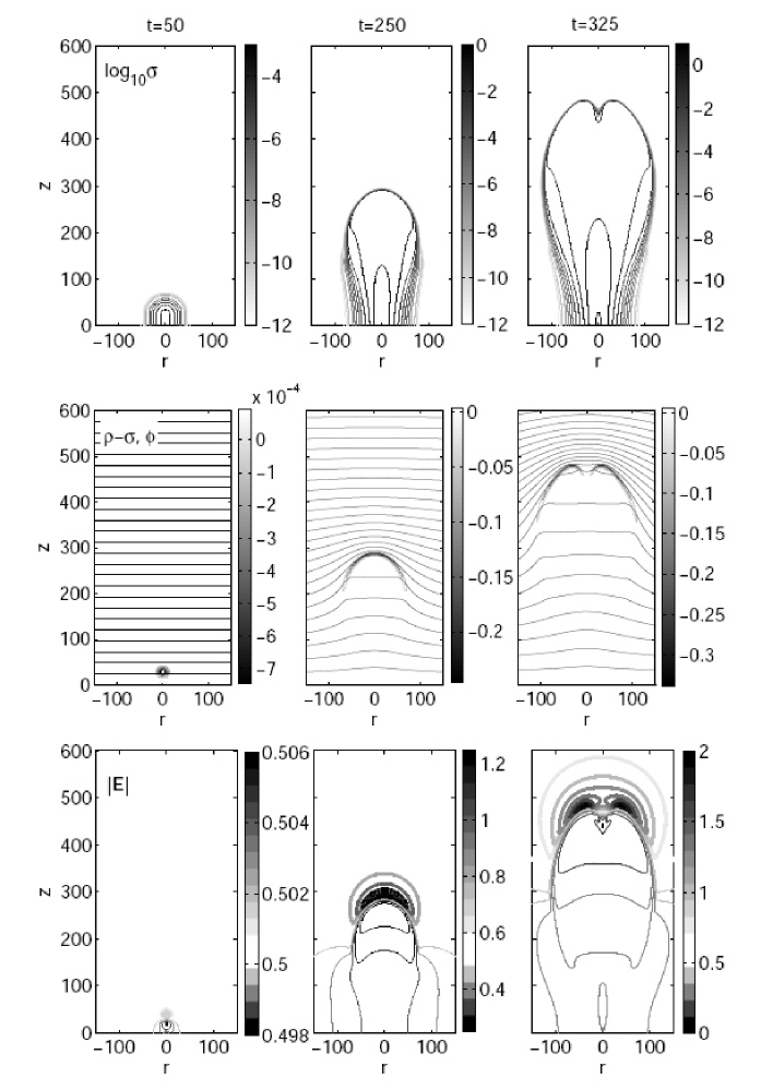
Figure 5: Evolution of the electron density distribution (upper row), net charge density and equipotential lines (middle row) and electric field strength (lower row), when an ionization seed attached to the cathode ($z$=0) is released in a background field of 0.5 in dimensionles units. The thick lines in the lower panel indicate where the field is higher than the background value, the thin lines where it is lower. The snapshots are taken at dimensionless times $t$=50, 250 and 325. Note that the quality and size of this figure (and some others) has been substantially reduced for the arxiv submission and will be better in the journal publication.

In the first column, a streamer just emerges from an avalanche. At this stage the space charges are smeared out over the complete streamer head and resemble very much the historical sketches of Raether [12] (cf. Fig. 10(a) below), as they also can be found in the textbooks of Loeb and Meek [13] or Raizer [69].

In the second column, the space charge region has contracted to a thin layer around the head, as also can be seen in many other studies of positive or negative streamers in nitrogen or air; now the electric field is suppressed in the ionized interior and substantially enhanced ahead of the streamer tip. As Raether’s estimate in [12] shows (cf. Fig. 10(a)), the field cannot be substantially enhanced in the initial stage of streamer evolution. However, it can in the second stage when the thin layer is formed. In this stage, the enhanced field in our calculation also easily can exceed the theoretical value suggested by Dyakonov and Kachorovskii [70, 71], and by Raizer and Simakov [72].

In the third column, the streamer head becomes unstable and branches. When we first published these results in [51], doubts were raised about the physical nature of the branching event [73, 74], refering also to an earlier debate of a similar observation [53, 75, 76]. This debate motivates our analysis and discussion in Section 5.

4.2 The multiscale nature of streamers

It is important to note the very different inherent scales of a propagating streamer, even within the minimal model. They are shown in Fig. 6: there is a wide non-ionized outer space where only the electrostatic Laplace equation $\nabla^{2}\phi=0$ has to be solved to determine the electric field. There are one or several streamer channels that are long and narrow. Around the streamer head, there is a layered structure with an ionization region and a screening space charge region.

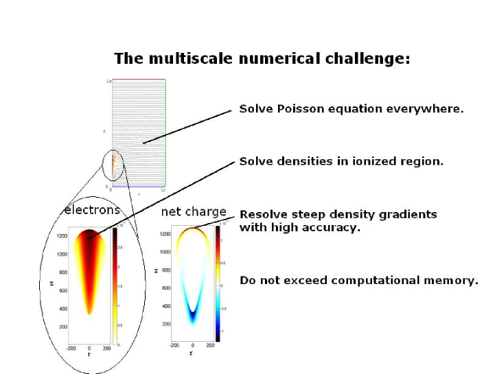
Figure 6: Sketch of the inherent scales of a propagating streamer.

Furthermore, in future work more regions should be distinguished: there is the leading edge of the front where the particle density is so low that the stochastic particle distribution leads to substantial fluctuations, and there is the interior ionized region where statistical fluctuations of particle densities are negligible: the characteristic number of charged particles within a characeristic volume $\alpha_{0}^{-3}$ is according to dimensional analysis

$$\frac{\epsilon_{0}\alpha_{0}{\cal E}_{0}}{\rm e}\cdot\alpha_{0}^{-3}\approx\frac{6000}{N/N_{0}}.$$ (9)

An immediate consequence is that stochastic density fluctuations are more important for high pressure discharges like streamers than for sprites. Whether this leads to different branching rates has to be investigated.

A large separation of length scales can be a benefit for analysis as it allows to use their ratios as small parameters and to develop a ladder of reduced models, see Section 5. On the other hand, it is a major challenge for numerical calculatioms.

4.3 Adaptive grid refinement

These numerical challenges can be met by adaptive grid refinement. Such a code has recently been constructed. It computes the evolution of a streamer on a relatively coarse grid and refines the mesh where the fine spatial structure of the solution requires. For preliminary and more extended results, we refer to [54, 66, 67, 68] and future papers. The distribution of the grid at different time steps is illustrated in Fig. 7. Here the evolution of a streamer in a long, undervolted gap is shown. More specifically, we consider a plane parallel electrode geometry, with an inter electrode distance of approximately 65000 in dimensionless units. The applied background electric field is uniform, and has a strength of 0.15. For N₂ under normal conditions this corresponds to a gap of about 15 cm with a background field of 30 kV/cm.

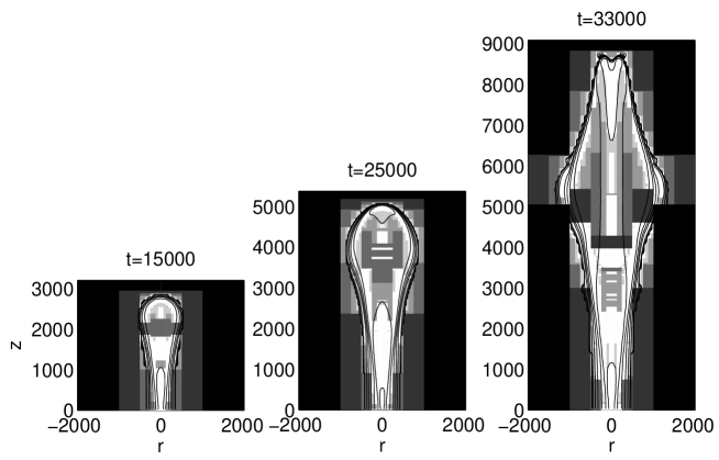
Figure 7: Evolution of the logarithm of the electron density together with the computational grids for a streamer evolving in a background field of 0.15, with an inter-electrode distance of approx. 65000. In pure molecular nitrogen under normal conditions this corresponds to a $\approx$15 cm gap with a background field of 30 kV/cm. The initial seed is attached to the cathode, allowing for a net electron inflow. The coarsest grid, in black, has a mesh size of 64, and is refined up to a mesh size of 2 (white domains).

We remark that the grid size used in the computation of the results shown in Fig. 7 is the same as that used by Vitello et al. [49] for a much smaller gap (0.5 cm) at a higher background field (50 kV/cm). In these simulations streamer branching was not seen, probably due to the shortness of the gap. On the contrary, a large gap as in the above examples enables the streamer to reach the instability even at a relatively low field.

Moreover, our previous calculations that showed streamer branching in a high background field of 0.5, were performed on a uniform numerical grid with grid spacing $\Delta x=2$ in [51] and with $\Delta x=1$ in [52]. We now are able to perform computations on a grid that adapts locally down to $\Delta x=1/8$ [67, 68].

For both background fields 0.5 and 0.15, the numerical results show that the time of streamer branching reaches a fixed value when using finer numerical meshes. We therefore conclude that streamer branching indeed is physical, and we will further support this statement with different arguments in the next section. We notice that in our cylindrically symmetric system, the streamer branches into rings, which obviously is rather unphysical. Therefore it is not meaningful to follow the further evolution of the streamer after branching. However, the effectively two-dimensional setting suppresses destablizing modes that break the cylindrical symmetry, and the time of branching in a cylindrically symmetric system therefore gives an upper bound for the branching time in the real three-dimensional system [74].

5 Analytical results on propagating and branching streamers

5.1 Nonlinear analysis of ionization fronts

The question of streamer branching can be addressed analytically, using concepts developed in other branches of science: Combustion, e.g., for decades is a very active area of applied nonlinear analysis, pattern formation and large scale computations. Chemical species are processed/burned when fuel is available and the temperature exceeds a threshold. The temperature is enhanced by the combustion front itself. Quite similarly, ionization is created is there are free electrons and if the electric field exceeds a threshold. The field is enhanced by the (curved) ionization front itself [64, 65, 51].

It is therefore attractive to develop analysis of streamers along the same lines, hence complementing numerical results with an analytical counterpart. This is particularly important for addressing questions of branching, long time evolution and multi-streamer structures. In particular, the structures of many interacting streamers in the near future will remain numerically inaccessible without model reduction.

5.2 The moving ionization boundary

In recent work, we have elaborated streamer evolution on two levels of refinement: the properties of a planar ionization front within the minimal model [64, 65, 51, 77], and the evolution of curved ionization boundaries [54, 78, 79]. A front solution is a solution of the full fluid model (3)–(5) zooming into the inner structure of the front. Ionization boundaries are formulated on the outer scale where the ionization front is reduced to a moving boundary between ionized and nonionized region.

If there is no initial ionization in the system, planar negative ionization fronts within the minimal model move with asymptotic velocity

$$v^{*}(E^{+})=|E^{+}|+2\sqrt{D\;f(|E^{+}|,\nu)}$$ (10)

into a field $E^{+}$ immediately ahead of the front. The degree of ionization $\sigma^{-}=\rho^{-}$ behind the front is a function of the field $E^{+}$. For large fields, the front velocity is dominated by the electron drift velocity $v^{*}(E^{+})\approx|E^{+}|$. For details about analyzing streamer fronts, we refer to [64, 65, 51, 77].

On the outer level of ionized and non-ionized region, a simple evolution model for the phase boundary can be formulated as shown in Fig. 8: assume the Lozansky Firsov approximation [80] that the streamer interior (indicated with an upper index ^-) is equipotential: $\phi^{-}=$ const. The exterior is free of space charges, hence $\nabla^{2}\phi^{+}=0$. Every piece of the boundary moves with the local velocity $v^{*}(E^{+})$ determined by the local field $E^{+}$ ahead of the front.

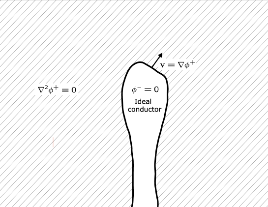
Figure 8: The moving boundary approximation for an ideally conducting streamer.

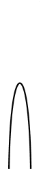
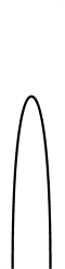
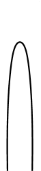
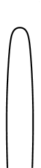
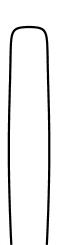
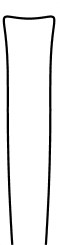
Figure 9: Temporal evolution of the streamer in the moving boundary approximation for an ideally conducting body, as shown in Fig. 8. The solution was computed assuming that the electric potential accross the ionization boundary is continuous $\phi^{-}=\phi^{+}$ and using conformal mapping methods [78].

If one assumes that the electric potential across the ionization boundary is continuous $\phi^{+}=\phi^{-}$ everywhere along the boundary, one arrives at a model that has been studied previously in the hydrodynamic context of viscous fingering. Our solutions of the model [54, 78] show that the transition from convex to concave streamer head indeed is dynamically possible (see Fig. 9); this is the onset of streamer branching. While these solutions demonstrate the onset of branching, they have the unphysical property that the local curvature of the boundary can become infinite within finite time. This cusp formation is suppressed in viscous fingering by a regularizing boundary condition. Our analysis [79] of streamer fronts suggests a new boundary condition

$$\phi^{+}-\phi^{-}=F(|E^{+}|),~{}~{}~{}F(|E^{+}|)\approx|E^{+}|~{}~{}~{}{\rm for}~{}|E^{+}|>2,$$ (11)

for the potential jump accross the boundary. This boundary condition aproximates the pde’s (3)–(5); it can be understood as a floating potential on the non-ionized side of the ionization boundary, if the potential on the ionized side is fixed. First results [79] with purely analytical methods indicate that this boundary condition indeed prevents cusp formation, i.e., it regularizes the problem.

We conclude that streamer branching is generic even for deterministic streamer models when they approach a state when the width of the space charge layer is much smaller than its radius of curvature, as in the second and third column of Fig. 5. A sketch of the distribution of surface charges and field is given by Fig. 8. A streamer in this state is likely to branch due to a Laplacian instability. A more precise characterization of the unstable state of the streamer head is under way.

5.3 How branching works and how it doesn’t

$\begin{array}[]{c}\includegraphics[height=128.0374pt]{psst10a.eps}\\ {\rm(a)}\\ \includegraphics[height=99.58464pt]{psst10b.eps}\\ {\rm(b)}\end{array}$

$\begin{array}[]{c}\includegraphics[height=156.49014pt]{psst10c.eps}\\ {\rm(c)}\end{array}$

Figure 10: (a) Space charge distribution in the emerging streamer head and (b) streamer propagation by photoionization according to Raether 1939 [12]. Fig. (b) was reproduced identically in [13] with English labels. Figure (c) shows the pictorial concept of streamer branching by rare and long-range photoionization events and successive avalanches as it can be found in many textbooks like [4]. It is a minor variation of Fig. b with the avalanches not aligned, but placed around the streamer head. The present version of the figure is taken from [11] where it motivates the dielectric breakdown model [10]. Find our critique of this concept in the text.

It came as a surprise to many that a fully deterministic model like our fluid model would exhibit branching, since another branching concept based on old pictures of Raether [12] is very well known. It is illustrated in Fig. 10. We remark on this concept:
1) The distribution and shape of avalanches ahead of the streamer head as shown in Fig. 10 c to the best of our knowledge have never been substantiated by further analysis.
2) Even if this avalanche distribution is realized, it has not been shown that it would evolve into several new streamer branches. Our major point of critique is that a space charge distributed over the full streamer head as in the figure would be self-stabilizing and not destabilizing, cf. a comparable recent analysis [81].

On the contrary, our main statement is: The formation of a thin space charge layer is necessary for streamer branching while stochastic fluctuations are not necessary.

Furthermore, for the question whether branching is possible in a deterministic fluid model, we remind the reader that chaos is possible in fully deterministic nonlinear models when their evolution approaches bifurcation points. Moreover, tip splitting in Laplacian growth problems as described in Fig. 8 is well established in viscous fingering in two fluid flow and other branches of physics.

5.4 The importance of charge transport and a remark on dielectric breakdown models

We have identified a state of the streamer head where it can branch. This state is characterized by a weakly curved ionization front, i.e., the radius of curvature is much larger than the width of the front. The width of the front is determined by the field $E^{+}$ ahead of it [65], for high fields the width saturates [65, 77]. The formation of such a weakly curved front requires a sufficiently high potential difference between streamer tip and distant electrode and an appropriate charge content of the streamer head. Charge is a conserved quantity. The consideration of charge conservation misses in the streamer concepts suggested in [70, 71, 72].

These considerations lead us to the general idea that a streamer tip is characterized by electric potential $\phi$, curvature $R$, field enhancement $E^{+}$ and total charge content $Q$. Only two of these four parameters are independent.

In contrast, dielectric barrier models (DBM) [10, 11] for multiply branched discharge structures are characterized only by potential and longitudinal spatial structure. We argue that a quantitative DBM model should also include the width of the streamer channel and the related charge content as a model variable. This would allow an appropriate characterization of streamer velocity and branching probability.

We remark that studies of streamer width and charge content are also crucial for determining the electrostatic interaction of streamers — or of leaders as their large relatives.

6 Summary and outlook

The purpose of the present paper was to review the presently available methods to investigate streamer discharges, in particular, those methods presently developed at TU Eindhoven and CWI Amsterdam. The paper summarizes a talk given at the XXVII’th International Conference on Phenomena in Ionized Gases (ICPIG) 2005.

Obviously, the complexity and the many scales of the phenomenon pose challenges to experiments, simulations, modeling and analytical theory if one wants to proceed to the quantitative understanding of more than a single non-branching streamer. In the present stage, we have developped reliable methods in each discipline, they are reviewed in the present paper. In the next stage, results of different methods should be compared: simulations should be compared with experiments, and simulations should be checked on consistency with analytical results. Analysis can also be used to extrapolate tediously generated numerical results, once the emergence of larger scale coherent structures — like complete streamer heads with their inner layers — has been demonstrated.

We have reviewed nanosecond resolved measurements of streamers and the surprising influence of the power supply, streamer applications and the relation to sprite discharges above thunderclouds. We have summarized the physical mechanisms of streamer formation and a minimal continuum density model that contains the essentials of the process. We have shown that a propagating and branching streamer even within the minimal continuum model consists of very different length scales that can be appropriately simulated with a newly developed numerical code with adaptive grids. Finally, we have summarized our present understanding of streamer branching as a Laplacian instability and compared it to earlier branching concepts.

On the experimental side, future tasks are precise measurements of streamer widths, velocities and branching characteristics and their dependence on gas type and power supply as well as quantitative comparison of streamers and sprites. On the theoretical side, both microscopic and macroscopic models should be developed further. Microscopically, the particle dynamics in the limited region of the ionization front will be investigated in more detail. Macroscopically, the quantitative understanding of streamer head dynamics should be incorporated into new dielectric breakdown models with predictive power. In particular, charge transport and conservation should be included. The theoretical tasks can only be treated succesfully, if a hierarchy of models on different length scales is developed: from the particle dynamics in the streamer ionization front up to the dynamics of a streamer head as whole. Elements of such a hierarchy are presented in the present paper.

Acknowledgements: This paper summarizes work by a number of researchers in a number of disciplines, therefore it has a number of authors. Beyond that, we acknowledge inspiration and thought exchange with the pattern formation group of Wim van Saarloos at Leiden Univ., with numerical mathematicians at cluster MAS at CWI Amsterdam, with colleagues in physics and electroengineering at TU Eindhoven, as well as with the many international colleagues and friends whom we met at conferences on gas discharges, atmospheric discharges and nonlinear dynamics in physics and applied mathematics. We thank Hans Stenbaek-Nielsen and Elisabeth Gerken for making sprite figures 3 and 4 available.

The experimental Ph.D. work of Tanja Briels in Eindhoven is supported by a Dutch technology grant (NWO-STW), the computational Ph.D. work of Carolynne Montijn is supported by the Computational Science program of FOM and GBE within NWO. The analytical Ph.D. work of Bernard Meulenbroek was supported by CWI. The postdoc position of Andrea Rocco was payed by FOM-projectruimte and the Dutch research school “Center for Plasma Physics and Radiation Technology” (CPS).

References

References

- [1] van Veldhuizen E M 2000 Electrical Discharges for Environmental Purposes: Fundamentals and Applications (Huntington, NY: Nova Science Publishers)
- [2] Bogaerts A, Neyts E, Gijbels R and van der Mullen J J A M 2002, Spectrochim. Acta B 57 609
- [3] Boeuf J-P, Lagmich Y and Pitchford L C 2005 Proc. XXVII Int. Conf. Phenomena in Ionized Gases (Eindhoven: The Netherlands) p 04-295
- [4] Bazelyan E M and Raizer Yu P 2000 Lightning Physics and Lightning Protection (Bristol: Institute of Physics Publishing)
- [5] Williams E R 2006 Plasma Sources Sci. Technol.[contribution in this volume].
- [6] Sentman D D, Wescott E M, Osborne D L and Heavner M J 1995 Geophys. Res. Lett. 22 1205
- [7] Gerken E A and Inan U S and Barrington-Leigh C P 2000 Geophys. Res. Lett. 27 2637
- [8] Pasko V P and Stenbaek-Nielsen H C 2002 Geophys. Res. Lett. 29 82
- [9] Pasko V P, Stanley M A, Mathews J D, Inan U S and Wood T G 2002, Nature 416 152
- [10] Niemeyer L, Pietronero L and Wiesman H J 1984 Phys. Rev. Lett.52 1033
- [11] Niemeyer L, Ullrich L and Wiegart N 1989 IEEE Trans. Electrical Insulation 24, 309
- [12] Raether H 1939 Z. Phys.112 464
- [13] Loeb L B and Meek J M 1941 The Mechanism of the Electric Spark (Stanford: Stanford University Press)
- [14] Wagner K H 1966 Z. Phys.189 465
- [15] Wagner K H 1967 Z. Phys.204 177
- [16] Chalmers I D, Duffy H and Tedford D J 1972 Proc. R. Soc. Lond. A 329 171
- [17] Creyghton Y L M 1994 Pulsed positive corona discharges, Ph.D. thesis, Eindhoven Universiy of Technology, The Netherlands
- [18] Blom P P M 1997, High-Power Pulsed Coronas, Ph.D. thesis, Eindhoven Universiy of Technology, The Netherlands
- [19] van Velduizen E M, Baede A H F M, Hayashi D and Rutgers W R 2001 APP Spring Meeting (Bad Honnef: Germany) p 231
- [20] van Veldhuizen E M, Kemps P C M and Rutgers W R 2002 IEEE Trans. Plasma Sci. 30 162
- [21] van Veldhuizen E M, Rutgers W T 2002 J. Phys. D: Appl. Phys.35 2169
- [22] van Veldhuizen E M, Rutgers W T and Ebert U 2002 Proc. XIV Int. Conf. Gas Discharges and their Appl. (Liverpool: England)
- [23] Yi W J and Williams P F 2002 J. Phys. D: Appl. Phys.35 205
- [24] Briels T M P, van Veldhuizen E M and Ebert U 2005 IEEE Trans. Plasma Sci. 33 264
- [25] Pancheshnyi S V, Nudovna M and Starikovskii A Y 2005 Phys. Rev. E 71 016407
- [26] Briels T M P, van Veldhuizen E M and Ebert U 2005 Proc. XXVII Int. Conf. Phenomena in Ionized Gases (Eindhoven: The Netherlands)
- [27] Grabowski L R, Briels T M P, van Veldhuizen E M and Pemen A J M 2005 Proc. XXVII Int. Conf. Phenomena in Ionized Gases (Eindhoven: The Netherlands)
- [28] Grabowski L R, van Veldhuizen E M and Rutgers W R 2005 J. Adv. Oxid. Technol. 8 142
- [29] Clements J S, Mizuno A, Finney W C and Davis R H 1989 IEEE Trans. Ind. Appl. 25 62
- [30] Dinelli G, Civitano L and Rea M 1990 IEEE Trans. Ind. Appl. 26 535
- [31] Clements J S, Sato M and Davis R H 1987 IEEE Trans. Ind. Appl. 23 224
- [32] Grymonpre, D R Sharma A K, Finney W C and Locke B R 2001 Chem. Eng. J. 82 189
- [33] Winands G J J, Yan K, Nair S A, Pemen A J M and van Heesch E J M 2005 Plasma Proc. and Polymers 2 232
- [34] Nair S A, Yan K, Pemen A J M, Winands G J J, van Gompel F M, van Leuken H E M, van Heesch E J M, Ptasinski K J and Drinkenburg A A H 2004 J. Electrostatics 61 117
- [35] Abou-Ghazala A, Katsuki S, Schoenbach K H, Dobbs F C and Moreira K R 2002 IEEE Trans. Plasma Sci. 30 1449
- [36] Rosocha L A, Coates D M, Platts D and Stange S 2004 Phys. Plasmas 11 2950
- [37] Krasnochub A V, Mintoussov E I, Nudnova M M and Starikovskii A Yu 2005 Proc. XXVII Int. Conf. on Phenom. in Ionized Gases (Eindhoven: The Netherlands) file 18-311
- [38] Starikovskii A 2005 private communication.
- [39] Klementeva I, Bocharov A, Bityurin V A and Klimov A 2005 Proc. XXVII Int. Conf. on Phenom. in Ionized Gases (Eindhoven: The Netherlands) file 05-444
- [40] Mazur V, Krehbiel P R and Shao X 1995 J. Geophys. Res. 100 25731
- [41] Franz R C, Nemzek R J and Winckler J R 1990 Science 249 48
- [42] Lyons W A 1996 J. Geophys. Res. 101 29641
- [43] Wescott E M, Sentman D D, Osborne D L and Heavner M J 1995 Geophys. Res. Lett. 22 1209
- [44] Wescott E M, Sentman D D, Heavner M J, Hampton D L and Vaughan Jr O H 1998 J. Atmos. Solar-Terr. Phys. 60 713
- [45] Neubert T 2003 Science 300 747
- [46] Stenbaek-Nielsen H C, Moudry D R, Wescott E M, Sentman D D and Sao Sabbas F T 2000 Geophys. Res. Lett. 27 3827
- [47] Stanley M, Krehbiel P, Brook M, Moore C, Rison W and Abrahams B 1999 Geophys. Res. Lett 26 pages 3201
- [48] Dhali S K and Williams P F 1987 J. Appl. Phys. 62 4696
- [49] Vitello P A, Penetrante B M and Bardsley J N 1994 Phys. Rev.E 49 5574
- [50] Babaeva N Yu and Naidis G V 1996 J. Phys. D: Appl. Phys.29 2423
- [51] Arrayás M, Ebert U and Hundsdorfer W 2002 Phys. Rev. Lett.88 174502
- [52] Rocco A, Ebert U and Hundsdorfer W 2002 Phys. Rev.E 66 035102(R)
- [53] Pancheshnyi S V and Starikovskii A Yu 2003 J. Phys. D: Appl. Phys.36 2683
- [54] Montijn C, Meulenbroek B, Ebert U and Hundsdorfer W 2005 IEEE Trans. Plasma Sci. 33 260
- [55] Qin B and Pedrow P D 1994 IEEE Trans. Dielect. Elect. Insulation 1 1104
- [56] Soria C, Pontiga F and Castellanos A 2001 J. Comp. Phys. 171 47
- [57] Pancheshnyi S V, Starikovskaia S M and Starikovskii A Yu 2001 J. Phys. D: Appl. Phys.34 105
- [58] Pancheshnyi S 2005 Plasma Sources Sci. Technol. 14 645
- [59] Davies A J and Evans C J 1967 Proc. IEE 114 1547
- [60] Morrow R and Lowke J J 1997 J. Phys. D: Appl. Phys.30 614
- [61] Kulikovsky A A 1998 Phys. Lett A 245 445
- [62] Liu N and Pasko V P 2004 J. Geophys. Res. 109 A04301
- [63] Liu N and Pasko V P 2006 J. Phys. D: Appl. Phys.39 327
- [64] Ebert U, van Saarloos W and Caroli C 1996 Phys. Rev. Lett.77 4178
- [65] Ebert U, van Saarloos W and Caroli C 1997 Phys. Rev.E 55 1530
- [66] Montijn C, Ebert U and Hundsdorfer W 2005 Proc. XXVII Int. Conf. Phenomena in Ionized Gases (Veldhoven: The Netherlands) 17-313
- [67] Montijn C, Ph.D. thesis, TU Eindhoven, Dec. 2005
- [68] Montijn C, Hundsdorfer W and Ebert U 2006 J. Comp. Phys. [to be accepted after revision], Preprint http://arxiv.org/abs/physics/0603070
- [69] Raizer Yu P 1991 Gas Discharge Physics (Berlin: Springer)
- [70] D’yakonov M I and Kachorovskii V Yu 1988 Sov. Phys. JETP 67 1049
- [71] D’yakonov M I and Kachorovskii V Yu 1989 Sov. Phys. JETP 68 1070
- [72] Raizer Yu P and Simakov A N 1998 PLasma Phys. Rep. 24 700
- [73] Kulikovsky A A 2002, Phys. Rev. Lett.89 229401
- [74] Ebert U and Hundsdorfer W 2002 Phys. Rev. Lett.89 229402
- [75] Kulikovsky A A 2000 J. Phys. D: Appl. Phys.33 1514
- [76] Pancheshnyi S V and Starikovskii A Yu 2001 J. Phys. D: Appl. Phys.34 248
- [77] Arrayás M and Ebert U 2004 Phys. Rev.E 69 036214
- [78] Meulenbroek B, Rocco A and Ebert U 2004 Phys. Rev.E 69 067402
- [79] Meulenbroek B, Ebert U and Schäfer L 2005 Phys. Rev. Lett.95 195004
- [80] Lozansky E D and Firsov O B 1973 J. Phys. D: Appl. Phys.6 976
- [81] Luiten O J, van der Geer S B, de Loos M J, Kiewiet F B and van der Wiel M J 2004 Phys. Rev. Lett 93 094802
- [82] Montijn C and Ebert U 2005 Diffusion correction to the avalanche–to–streamer transition Preprint http://arxiv.org/abs/physics/0508109