A Qualitative Description of Boundary Layer Wind Speed Records

Abstract

The complexity of the atmosphere endows it with the property of turbulence by virtue of which, wind speed variations in the atmospheric boundary layer (ABL) exhibit highly irregular fluctuations that persist over a wide range of temporal and spatial scales. Despite the large and significant body of work on microscale turbulence, understanding the statistics of atmospheric wind speed variations has proved to be elusive and challenging. Knowledge about the nature of wind speed at ABL has far reaching impact on several fields of research such as meteorology, hydrology, agriculture, pollutant dispersion, and more importantly wind energy generation. In the present study, temporal wind speed records from twenty eight stations distributed through out the state of North Dakota (ND, USA), ($\sim$ 70,000 square-miles) and spanning a period of nearly eight years are analyzed. We show that these records exhibit a characteristic broad multifractal spectrum irrespective of the geographical location and topography. The rapid progression of air masses with distinct qualitative characteristics originating from Polar regions, Gulf of Mexico and Northern Pacific account for irregular changes in the local weather system in ND. We hypothesize that one of the primary reasons for the observed multifractal structure could be the irregular recurrence and confluence of these three air masses.

keywords : wind speed, self-similarity, multifractal scaling, atmosphere, boundary layer

1 Introduction

Atmospheric phenomena are accompanied by variations at spatial and temporal scales. In the present study, qualitative aspects of temporal wind speed data recorded at an altitude of 10 ft from the earth’s surface are discussed. Such recordings fall under the ABL, which is the region 1-2 km from the earths surface [1]. Flows in the ABL, which are generally known to be turbulent, are influenced by a number of factors including shearing stresses, convective instabilities, surface friction and topography [1, 2]. The study of laboratory scale turbulent velocity fields has received a lot of attention in the past (see [3] for a summary). A. N. Kolmogorov [4, 5], (K41) proposed a similarity theory where energy in the inertial sub-range is cascaded from the larger to smaller eddies under the assumption of local isotropy. For the same, K41 statistics is also termed as small-scale turbulence statistics. The seminal work of Kolmogorov encouraged researchers to investigate scaling properties of turbulent velocity fields using the concepts of fractals [6]. Subsequent works of Parisi and Frisch [7], Meneveau and Srinivasan, [8, 9, 10] provided a multifractal description of turbulent velocity fields. While there has been a precedence of scaling behavior in turbulence at microscopic scales [4, 5, 6, 7, 8, 9, 10, 11] it is not necessary that such a scaling manifest itself at macroscopic scales, although there have been indications of “unified scaling” models of atmospheric dynamics, [12]. Several factors can significantly affect the behavior of a complex system such as ABL [2, 1]. Thus, an extension of these earlier findings [4, 5, 6, 7, 8, 9, 10, 11] to the present study is neither immediate, nor obvious. Attempts have also been made to simulate the behavior of the ABL [13, 14]. However, there are implicit assumptions made in these studies and often, there can be significant discrepancies between simulated flows and the actual phenomenon when these assumptions are violated [3]. On the other hand, knowledge about the nature of wind speed at ABL has far reaching impact on several fields of research. In particular, the need to obtain accurate statistical descriptions of flows in the ABL from actual site recordings is both urgent and important, given its utility in the planning, design and efficient operation of wind turbines, [15]. Therefore, analysis of wind speed records based on numerical techniques is gaining importance in the recent years. In [16], long term daily records of wind speed and direction were represented as a two dimensional random walk and the results reinforce the important role that memory effects have on the dynamics of complex systems. In [17], the short term memory of recorded surface wind speed records is utilized to build $m$’th order Markov chain models, from which probabilistic forecasts of short time wind gusts are made. In [18], the authors study the correlations in wind speed data sets over a span of 24 hours, using detrended fluctuation analysis (DFA), [19] and its extension, multifractal-DFA (MF-DFA)[20]. Their studies show that the records display long range correlations with a fluctuation exponent of $\alpha\sim 1.1$ along with a broad multifractal spectrum. In addition, they also suggest the need for detailed analysis of data sets from several other stations to ascertain whether such features are characteristic of wind speed records. In [21], it is shown that rare events such as wind gusts in wind speed data sets that are long range correlated are themselves long range correlated. In [22], it is shown that surface layer wind speed records can be characterized by multiplicative cascade models with different scaling relations in the microscale inertial range and the mesoscale. Our previous studies, [23] suggest that at short time scales, hourly average wind speed records are characterized by a scaling exponent $\alpha\sim 1.4$ and at large time scales, by an exponent of $\alpha\sim 0.7$. A deeper examination of the data sets in [26] using MF-DFA indicated that the records also admitted a broad multifractal spectrum under the assumption of a binomial multiplicative cascade model. Interestingly, scaling phenomena have also been found in fluctuations of meteorological variables that influence wind speed such as air humidity, [24], temperature records and precipitation [25]. In [25], it is observed that while temperature records display long range correlations ($\alpha\sim 0.7$), they do not display a broad multifractal spectrum. On the other hand, precipitation records display a very weak degree of correlation with ($\alpha\sim 0.5$, [25]). While it is difficult to directly relate the scaling results of these variables to that of wind speed, greater insight can be gained by analyzing data sets that are recorded over long spans from different meteorological stations. Motivated by these findings, we chose to investigate the temporal aspects of wind speed records dispersed over a wide geographical area. In the present study, we follow a systematic approach in determining the nature of the scaling of wind speed records recorded at an altitude of 10 ft across 28 spatially separated locations spanning an area of approximately 70,000 sq.mi and recorded over a period of nearly 8 years in the state of North Dakota.

As noted earlier, convective instabilities and topography can have a prominent impact of the flow in ABL. The air motion over North Dakota is governed by the flow of three distinct air masses with distinct qualities, namely from : (i) the polar regions to the north (cold and dry) (ii) the Gulf of Mexico to the south (warm and moist) and (iii) the northern pacific region (mild and dry). The rapid progression and interaction of these air masses results in the region being subject to considerable climactic variability. These in turn can have a significant impact on the convective instabilities which governs the flow in ABL. On the other hand, the topography of the region has sharp contrasts on the eastern and western parts of the state because of their approximate separation by the boundary of continental glaciation. The eastern regions have a soft topography compared to the western region which comprises mostly of rugged bedrock. In the present study, we show that the qualitative characteristics of the wind speed records do not change across the spatially separated locations despite the contrasting topography. This leads us to hypothesize that the confluence of the air masses as opposed to the topography plays a primary role in governing the wind dynamics over ND.

2 Methods

Spectral analysis of stationary processes is related to correlations in it by the Wiener-Khinchin theorem, [27] and has been used for detecting possible long-range correlations. In the present study, we observed broad-band power-law decay superimposed with peaks. This spectral signature was consistent across all the 28 stations (Fig. 1(b)). Such power-law processes lack well-defined scales and have been attributed to self-organized criticality, intermittency, self-similarity [28, 29] and multiscale randomness [30]. Superimposed on the power-law spectrum, were two high frequency peaks which occur at $t_{1}=24$ and $t_{2}=12$ hours corresponding to diurnal and semi-diurnal cycles respectively.

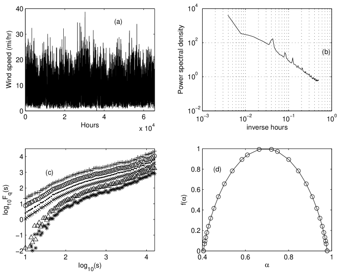
Figure 1: (a) Temporal trace of hourly average wind speed record (miles/hour) at one of the representative stations (Baker 1N, refer to Table 1 for details) over a period of nearly 8 years. (b) The corresponding power spectrum exhibits a power law decay of the form ($S(f)\sim 1/f^{\beta}$). Superimposed on the power spectrum are prominent peaks which correspond to multiple sinusoidal trends. (c) Log-Log plots of the fluctuation function versus time scale, $F_{q}(s)\;$vs$\;s$ for the moments $q=-10($*$)$, -6 (triangle ), -0.2$(\times)$ , 2 (.), 6$(\circ)$ and $q=10(+)$ (d) Multifractal spectrum of the record determined under the assumption of a binomial multiplicative cascade model.

Power-law decay of the power-spectrum (Fig. 1(b)) can provide cues to possible long-range correlations, but, however, it is susceptible to trends and non-stationarities which are ubiquitous in recordings of natural phenomena. While several estimators [31, 32] have been proposed in the past for determining the scaling exponents from the given data, detrended fluctuation analysis (DFA), [19] and its extension, generalized multifractal-DFA (MF-DFA)[20] have been widely used to determine the nature of the scaling in data obtained from diverse settings [20, 33, 34, 35, 36]. In DFA, the scaling exponent for the given monofractal data is determined from least-squares fit to the log-log plot of the second-order fluctuation functions versus the time-scale, i.e. $F_{q}(s)\;$vs$\;s$ where $q=2$. For MF-DFA, the variation of the fluctuation function with time scale is determined for varying $q\;(q\neq 0$). The superiority of DFA and MF-DFA to other estimators along with a complete description is discussed elsewhere [33]. DFA and MF-DFA procedures follow a differencing approach that can be useful in eliminating local trends [19]. However, recent studies have indicated the susceptibility of DFA and MF-DFA to higher order polynomial trends. Subsequently, DFA-$n$ [37] was proposed to eliminate polynomial trends up to order $n-1$. In the present, study we have used polynomial detrending of order four. However, such an approach might not be sufficient to remove sinusoidal trends which can be periodic [39] or quasiperiodic (see discussion in Appendix A).

Data sets spanning a number of years, as discussed here, are susceptible to seasonal trends that can be periodic or quasiperiodic in nature. Such trends manifest themselves as peaks in the power spectrum and their power is a fraction of the broad-band noise. These trends can also introduce spurious crossovers as reflected by log-log plot of $F_{q}(s)\;$vs$\;s$ and prevent reliable estimation of the scaling exponent. Such crossovers indicate spurious existence of multiple scaling exponents at different scales and shift towards higher time scales with increasing order of polynomial detrending [37]. Thus, it is important to discern correlations that are an outcome of trends from those of the power-law noise. In a recent study, [38], a singular-value decomposition (SVD) based approach was proposed to minimize the effect of the various types of trends superimposed on long-range correlated noise. However, SVD is a linear transform and may be susceptible when linearity assumptions are violated. Therefore, we provide a qualitative argument to identify multifractality in wind speed records superimposed with periodic and/or quasiperiodic trends. Multifractality is reflected by a change in the slope of the log-log fluctuation plots with varying $q$ with $(q\neq 0)$ [20]. For a fixed $q$, one observes spurious crossovers in monofractals well as multifractal data sets superimposed sinusoidal trends. Thus nonlinearity or a crossover of the log-log plot for a fixed $q$ might be due to trends as opposed to the existence of multiple scaling exponents at different scales. However, we show (see discussion under Appendix A) that the nature of log-log plot of $F_{q}(s)\;$vs$\;s$ does not change with varying $q$ for monofractal data superimposed with sinusoidal trends. However, a marked change in the nature if the log-log plots $F_{q}(s)\;$vs$\;s$ with varying $q$ is observed for multifractal data superimposed with trends. Therefore, in the present study, the log-log plot of $F_{q}(s)$ vs $s$ with varying $q$ is used as a qualitative description of multifractal structure in the given data. For the wind-speed records across the 28 stations, we found the peaks in the power spectrum to be consistent across all the 28 stations. Thus any effects due to the trend on the multifractal structure, we believe would be consistent across the 28 stations.

3 Results

MF-DFA was applied to the data sets recorded at the 28 stations. The log-log plots of the fluctuation functions ($F_{q}(s)\;$ vs $\;s$) with varying moments $q$ = -10, -6, -0.2, 2, 6, 10) using fourth order polynomial detrending for one of the representative records is shown in Fig.1(c). From Fig.1(c), it can be observed that the data sets exhibit different scaling behavior with varying $q$, characteristic of a multifractal process. This has to be contrasted with monofractal data whose scaling behavior is indifferent to the choice of $q$ in the presence or absence of sinusoidal trends.

To compute the $q$ dependence of the scaling exponent $h(q)$, we select the time scale in the range [2.2 - 3.7] where the scaling was more or less constant for a given $q$. Note that this corresponds to variations in a time span of $[10^{2.2}-10^{3.7}]\sim[158-5012]$ hours, for a given $q$. In this range, the slope of the fluctuation curves $h(q)$ was calculated for every $q$ and for ever station. The mean of the generalized exponents $h(q)$ over all the twenty eight stations along with the standard deviation bars are shown in Fig. 2(a).

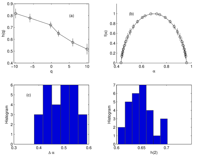
Figure 2: (a) The mean (circle) and the standard deviation (vertical lines) of the generalized Hurst exponent, $h(q)$ vs $q$ across the 28 stations (b) The mean (circle) and the standard deviation (vertical lines) of the multifractal spectrum $f(\alpha)$ across the 28 stations. (c) Histogram of the multifractal widths $(\Delta\alpha)$ across the 28 stations (d) Histogram of the Hurst exponent $h(2)$.

It can be noted from Fig. 2(a) that the slopes $h(q)$ decrease as the moment $q$ varies from negative to positive values which signifies that wind speed fluctuations are heterogeneous and thus, a range of exponents is necessary to completely describe their scaling properties. To capture this notion of multifractality, we estimate the classical Renyi exponents $\tau(q)$ and the singularity spectrum [40] under the assumption of binomial multiplicative process [41, 40, 20] (see Appendix A for details). The singularity spectrum of one of the representative stations (Baker, 1N) is shown in Fig.1(d) and its variation across the 28 stations is shown in Fig. 2(b). The fitting parameters $a,b$ for the cascade model, the Hurst exponent $h(2)$ and the multifractal width $\Delta\alpha$ for all the stations are summarized in Table 1.

Table 1: Names and locations of the 28 recording stations. The fitting parameters $(a,b)$ of the cascade model, the Hurst exponent $h(2)$ and the multifractal width $(\Delta\alpha)$ are also indicted.

Station Number	Name	$a$	$b$	$h(2)$	$\Delta\alpha$
1	Baker 1N	0.513	0.710	0.702	0.469
2	Beach 9S	0.523	0.76	0.643	0.539
3	Bottineau 14W	0.525	0.720	0.699	0.456
4	Carrington 4N	0.521	0.721	0.638	0.468
5	Dazey 2E	0.551	0.722	0.609	0.390
6	Dickinson 1NW	0.535	0.715	0.670	0.418
7	Edgeley 4SW	0.531	0.752	0.573	0.510
8	Fargo 1NW	0.505	0.719	0.641	0.510
9	Forest River 7WSW	0.556	0.739	0.670	0.411
10	Grand Forks 3S	0.527	0.757	0.646	0.522
11	Hazen 2W	0.544	0.733	0.672	0.430
12	Hettinger 1NW	0.523	0.748	0.610	0.516
13	Hillsboro 7SE	0.522	0.751	0.620	0.526
14	Jamestown 10 W	0.547	0.739	0.636	0.434
15	Langdon 1E	0.545	0.710	0.644	0.381
16	Linton 5N	0.531	0.711	0.623	0.422
17	Minot 4S	0.550	0.706	0.629	0.459
18	Oakes 4S	0.507	0.755	0.657	0.574
19	Prosper 5NW	0.504	0.720	0.671	0.513
20	Mohall 1W	0.513	0.753	0.654	0.554
21	Streeter 6NW	0.521	0.742	0.675	0.509
22	Turtle Lake 4N	0.546	0.729	0.693	0.418
23	Watford City 1W	0.524	0.768	0.631	0.551
24	St. Thomas 2WSW	0.550	0.744	0.633	0.434
25	Sidney 1NW	0.518	0.772	0.635	0.593
26	Cavalier 5W	0.506	0.736	0.651	0.539
27	Williston 5SW	0.514	0.759	0.635	0.562
28	Robinson 3NNW	0.514	0.739	0.620	0.525

These results indicate multifractal scaling consistent across the stations. Earlier studies [42, 43, 20] have suggested the choice of random shuffled surrogates to rule out the possibility that the observed fractal structure is due to correlations as opposed to broad probability distribution function. The wind speeds in the present study follow a two-parameter asymmetric Weibull distribution whose parameters were also similar across the 28 stations. MF-DFA on the random shuffle surrogates of the original records Fig.2(d) indicate a scaling of the form $F_{q}(s)\sim s^{0.5}$ with varying $q$, characteristic of random noise and loss of multifractal structure. The width of the multifractal spectrum was used to characterize the strength of multifractality. The histogram of the multifractal widths obtained across the 28 stations, Fig. 2(c), was narrow with mean and standard deviation $\Delta(\alpha)=(0.4866\pm 0.0599)$. The multifractal widths and the Hurst exponent $h(2)$ across the twenty eight stations is also shown in Fig.3.

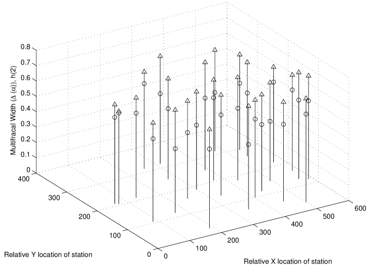
Figure 3: The multifractal width for each of the 28 stations is indicated by circles. The Hurst exponent $h(2)$ is indicated by upright triangles. The x-y plane represents the x and y coordinate in the of North Dakota.

In the present study a systematic approach was used to determine possible scaling in the temporal wind-speed records over 28 spatially separated stations in the state of North Dakota. Despite the spatial expanse and contrasting topography the multifractal qualitative characteristics of the wind speed records as reflected by singularity spectrum, were found to be similar. Thus multifractality may be an invariant feature in describing the dynamics long-term motion of wind speed records in ABL over North Dakota. We also believe that the irregular recurrence and confluence of the air masses from Polar, Gulf of Mexico and the northern Pacific may play an important role in explaining the observed multifractal structure.

Appendix A Data Acquisition, MF-DFA algorithm and Discussion

A.1 Data Acquisition

The wind speed records at the 28 stations spanning nearly 8 years were obtained from part of the climatological archives of the state of North Dakota. Stations were selected to represent the general climate of the surrounding area. Wind speeds were recorded by means of conventional cup type anemometers located at a height of 10 ft. The anemometers have a range of 0 to 100 mph with an accuracy of $\pm 0.25$ mph. Wind speeds acquired every five seconds are averaged over a 10 minute interval to compute the 10 minute average wind speed. The 10 minute average wind speeds are further averaged over a period of one hour to obtain the hourly average wind speed.

A.2 Multifractal Detrended Fluctuation Analysis (MF-DFA):

MF-DFA, [20] a generalization of DFA has been shown to reliably extract more than one scaling exponent from a time series. A brief description of the algorithm is provided here for completeness. A detailed explanation can be found elsewhere [20]. Consider a time series $\{x_{k}\},k=1\dots N$. The MF-DFA algorithm consists of the following steps.

1. The series $\{x_{k}\}$ is integrated to form the integrated series $\{y_{k}\}$ given by

   $$y(k)=\sum_{i=1}^{i=k}[x(i)-\bar{x}]\;\;\;k=1,\dots N$$ (1)

   where $\bar{x}$ represents the average value.

2. The series $\{y_{k}\}$ is divided in to $n_{s}$ non-overlapping boxes of equal length$s$ where $n_{s}=int(N/s)$. To accommodate the fact that some of the data points may be left out, the procedure is repeated from the other end of the data set [20].

3. The local polynomial trend $y_{v}$ with order $v$ is fit to the data in each box, the corresponding variance is given by

   $$F^{2}(v,s)=\left\{\frac{1}{s}\sum_{i=1}^{i=s}\{y[N-(v-n_{s})s+i]-y_{v}(i)\right\}^{2}$$ (2)

   for $v=1,\dots n_{s}$. Polynomial detrending of order m is capable of eliminating trends up to order m-1. [20]

4. The $qth$ order fluctuation function is calculated from averaging over all segments.

   $$F_{q}(s)=\left\{\frac{1}{2n_{s}}\sum_{i=1}^{i=2n_{s}}[F^{2}(v,s)]^{q/2}\right\}^{1/q}$$ (3)

   In general, the index $q$ can take any real value except zero.

5. Step 3 is repeated over various time scales $s$. The scaling of the fluctuation functions $F_{q}(s)$ versus the time scale $s$ is revealed by the log-log plot.

6. The scaling behavior of the fluctuation functions is determined by analyzing the log-log plots $F_{q}(s)$ versus $s$ for each $q$. If the original series $\{x_{k}\}$ is power-law correlated, the fluctuation function will vary as

   $$F_{q}(s)\sim s^{h(q)}$$ (4)

The MF-DFA algorithm [20] was used to compute the multifractal fluctuation functions. The slopes of the fluctuation functions ($h(q)$) for each
$q=(-10,-6,-0.2,2,6,10)$ was estimated by linear regression over the time scale range $s=[2.2,3.7]$. The generalized Hurst exponents ($h(q)$) are related to the Renyi exponents $\tau(q)$ by $qh(q)=\tau(q)+1$. The multifractal spectrum $f(\alpha_{h})$ defined by, [40] $\alpha_{h}=\frac{d\tau(q)}{dq},\;\;f(\alpha_{h})=q\alpha_{h}-\tau(q)$. Under the assumption of a binomial multiplicative cascade model [40] the generalized exponents $h(q)$ can be determined from $h(q)=\frac{1}{q}-\frac{ln(a^{q}+b^{q})}{qln2}$. The parameters $a$ and $b$ for each station was determined using a nonlinear least squares fit of the preceding formula with those calculated numerically. Finally, the multifractal width was calculated using $\Delta\alpha=\Delta\alpha_{h}=h(-\infty)-h(\infty)=\frac{(ln(b)-ln(a))}{ln2}$, [20].

A.3 Discussion

The power spectrum of the wind speed records considered in the present study exhibited a power law decay of the form ($S(f)\sim 1/f^{\beta}$) superimposed with prominent peaks which corresponds to multiple sinusoidal trends. Such a behavior is to expected on data sets spanning several years. The nature of the power spectral signature was consistent across all stations. This enables us to compare the nature of scaling across the 28 stations. Recent studies had indicated the susceptibility of MF-DFA to sinusoidal trends in the given data, [39]. Sinusoidal trends can give rise to spurious crossovers and nonlinearity in the log-log plot that indicate the existence of more than one scaling exponent. In a recent study [38], we had successfully used the singular-value decomposition to minimize the effect of offset, power-law, periodic and quasi-periodic trends. However, SVD is a linear transform and may be susceptible when linearity assumptions are violated. Estimating the SVD for large-embedding matrices is computationally challenging. Therefore, in the present study we opted for a qualitative description of multifractal structure by inspecting the nature of the log-log plots of the fluctuation function versus time scale $F_{q}(s)\;$vs $\;s$ with varying moments $q$. We show that the nature of the log-log plot does not show appreciable change with varying moments $q$ for monofractal data superimposed with sinusoidal trends. However, a marked change in the nature of the log-log plot is observed for multifractal data superimposed with sinusoidal trends. Moreover, the nature of the trends as reflected by the power spectrum is consistent across the 28 stations. This enables us to compare the multifractal description obtained across the stations. The effectiveness of the qualitative description is demonstrated with synthetic monofractal and multifractal data sets superimposed with sinusoidal trends.

A.3.1 MF-DFA results of monofractal and multifractal data superimposed with sinusoidal trends

Consider a signal $y_{1}(n)$ consisting of monofractal data $s_{1}(n)$ superimposed with a sinusoidal trend $t_{1}(n)$. Let $y_{2}(n)$ be a signal consisting of multifractal data $s_{2}(n)$ superimposed with sinusoidal trend $t_{2}(n)$. The trends are described by,

$$t_{1}(n)=A_{1}\sin(2\pi n/T_{1})+A_{2}\sin(2\pi n/T_{2})+A_{3}\sin(2\pi n/T_{3}),n=1\dots N_{1}$$

$$t_{2}(n)=B_{1}\sin(2\pi n/T_{1b})+B_{2}\sin(2\pi n/T_{2b}),n=1\dots N_{2}$$

The signals are given by, $y_{i}(n)=s_{i}(n)+t_{i}(n),i=1,2$ where $s_{1}(n)$ is monofractal data with $\alpha=0.9$ and $s_{2}(n)$ is multifractal data is that of internet log traffic, [44]. The dominant spectral peaks Fig.4(a) and Fig.4(b) reflect the presence of these trends in signals $y_{1}$ and $y_{2}$ respectively. The MF-DFA plots $F_{q}(s)\;$ vs $\;s$ with fourth order detrending and $q=-10,-8,-6,-4,-2,2,4,6,8,10$ for signals $y_{1}$ and $y_{2}$ are shown in Fig.4(c) and Fig.4(d) respectively. For the monofractal data, the trends introduce spurious crossover at $s\sim 2.2$ in the log-log plot of the $F_{q}(s)\;$vs $\;s$ for a given $q$. However, the nature of the log-log plots fail to show appreciable change with varying $q$, Fig.4(c). For multifractal data with trends, spurious crossovers are still noted at $s\sim 2.2$ in the log-log plot of the $F_{q}(s)\;$vs $\;s$ for a given $q$. However, in this case, Fig.4(d), the nature of the log-log plots show a significant change with varying $q$ indicating multifractal scaling in the given data, unlike the case with monofractal data with trends.

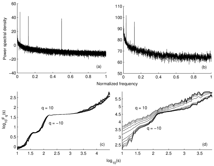
Figure 4: MF-DFA studies of monofractal and multifractal data sets superimposed with multiple sinusoidal trends.

Parameters:

$A_{1}=6,\;A_{2}=3,\;A_{3}=2,\;T_{1}=2^{6},\;T_{2}=2^{4},\;T_{3}=2^{2},N_{1}=2^{17},\;B_{1}=6000,\;B_{2}=3000,\;T_{1b}=2^{6},\;T_{2b}=2^{4},N_{2}=2^{15}$.

The data sets are available from
http://www.physionet.org/physiobank/database/synthetic/tns/.

References

- [1] J. R. Garratt, The Atmospheric Boundary Layer, Cambridge Univ. Press, (1994).
- [2] A. A. Monin and A. M. Obukhov, Basic laws of turbulent mixing in the ground layer of the atmosphere, Trans. Geophys. Inst. Akad. Nauk. USSR 151, 163-187, (1954).
- [3] Z. Warhaft, Turbulence in nature and in the laboratory, PNAS 99, 2481-2486, (2002).
- [4] A. N. Kolmogorov, The local structure of turbulence in incompressible viscous fluid for very large Reynolds numbers, Dokl. Acad. Nauk. SSSR 30, 301-305, (1941).
- [5] A. N. Kolmogorov, Dissipation of energy in the locally isotropic turbulence, Dokl. Akad. Nauk. SSSR 31, 538-540, (1941).
- [6] B. Mandelbrot, Intermittent turbulence in self-similar cascades : divergence of high moments and dimension of the carrier, J. Fluid Mech. 62, 331-358, (1974).
- [7] G. Parisi and U. Frisch, On the singularity structure of fully developed turbulence, Turbulence and Predictability in Geophysical Fluid Dynamics and Climate Dynamics. (eds: M. Ghil, R. Benzi and G. Parisi) 71, (1985).
- [8] C. Meneveau and K. R. Sreenivasan, Simple multifractal cascade model for fully developed turbulence, Phy. Rev. Lett 59, 1424-1427, (1987).
- [9] C. Meneveau and K. R. Sreenivasan, The multifractal spectrum of the dissipation field in turbulent flows, Nuclear Physics B (Proc. Suppl.) 2, 49-76, (1987).
- [10] C. Meneveau and K. R. Sreenivasan, The multifractal nature of turbulent energy dissipation, Journal of Fluid Mechanics 224, 429-484, (1991)
- [11] F. Argoul, Wavelet analysis of turbulence reveals the multifractal nature of the Richardson cascade, Nature 338, 51-53, (1989).
- [12] S. Lovejoy, D. Schertzer and J. D. Stanway, Direct evidence of multifractal atmospheric cascades from planetary scales down to 1 km, Phy. Rev. Lett 86, 5200-5203, (2001).
- [13] F. Ding, S. Pal Arya and Y. L. Lin, Large eddy simulations of atmospheric boundary layer using a new sub-grid scale model, Environmental Fluid Mechanics 1, 49-69, (2001).
- [14] C-H. Moeg, A large eddy simulation model for the study of planetary boundary layer, J. Atmos. Sci. 41, 2052-2062, (1984).
- [15] J. Peinke, S. Barth, F. Bottcher, D. Heinemann and B. Lange, Turbulence, a challenging problem for wind energy, Physica A, 338, 187-193, (2004).
- [16] B. M. Schulz, M. Schulz and S. Trimper, Wind direction and strength as a two dimensional random walk, Physics Letters A, 291, 87-91, (2001).
- [17] H. Kantz, D. Holstein, M. Ragwitz and N. K. Vitanov, Markov chain model for turbulent wind speed data, Physica A, 342, 315-321, (2004).
- [18] R. B. Govindan and H. Kantz, Long term correlations and multifractality in surface wind, Europhysics Letters, 68, 184-190, (2004).
- [19] C. K. Peng et.al., Mosaic organization of DNA nucleotides, Phys. Rev. E 49, 1685-1689, (1994)
- [20] J. W. Kantelhardt, S. A. Zschiegner, S. Havlin, A. Bunde and H. E. Stanley, Multifractal detrended fluctuation analysis of nonstationary time series, Physica A 316, 87-114, (2002).
- [21] M. S. Santhanam and H. Kantz, Long range correlations and rare events in boundary layer wind fields, Physica A, 345, 713-721, (2005).
- [22] M. K. Lauren, M. Menabde and G. L. Austin, Analysis and simulation of surface layer winds using multiplicative cascaded models with self similar probability densities, Boundary Layer Meteorology, 100, 263-286, (2001).
- [23] R. G. Kavasseri and R. Nagarajan, Evidence of crossover phenomena in wind speed data, IEEE Trans. on Circuits and Systems. Fundam. Theory and Apps. 51(11), 2251 - 2262, (2004).
- [24] G. Vattay and A. Harnos, Physical Review Letters, Scaling behavior in daily air humidity fluctuations, 73(5), 768-771, 1994.
- [25] A. Bunde, J. Eichner, R. Govindan, S. Havlin, E. K. Bunde, D. Rybski and D. Vjushin, Power law persistence in the atmosphere : analysis and applications, In Nonextensive Entropy - Interdisciplinary Applications - edited by M. Gell-Mann and C. Tsallis, New York Oxford University Press, (2003).
- [26] R. G. Kavasseri and R. Nagarajan, A multifractal description of wind speed records, Chaos, Solitons and Fractals, vol. 24, No.1, 165 - 173, (2005).
- [27] A. Papoulis, Random Variables and Stochastic Processes, Mc Graw Hill (1994).
- [28] P. Bak, C. Tang and K. Wiesenfeld, Self-organized criticality: an explanation of 1/f Noise, Phys. Rev. Lett. 59, 381-384, (1987).
- [29] P. Manneville, Intermittency, self-similarity and 1/f spectrum in dissipative dynamical systems, Journal de Physique 41, 1235-1243, (1980).
- [30] J. M. Haussdorf and C-K. Peng, Multiscaled randomness: A possible source of 1/f scaling in biology, Physical Review E 54, 2154-2157, (1994).
- [31] H. E. Hurst, Long-term storage capacity of reservoirs, Trans. Amer. Soc. Civ. Engrs. 116, 770-808, (1951)
- [32] P. Abry and D. Veitch, Wavelet analysis of long-range-dependent traffic, IEEE Trans. on Information Theory 44, 2-15, (1998).
- [33] J. W. Kantelhardt et.al, Multifractality of river runoff and precipitation: Comparison of fluctuation analysis and wavelet methods, Physica A 33, 240-245, (2003)
- [34] V. Livina et.al, Physica A 330, 283-290, (2003).
- [35] S. Havlin et.al, Physica A 274, 99-110, (1999).
- [36] Y. Ashkenazy et.al, Phy. Rev. Lett 86, 1900-1903, (2001).
- [37] J. W. Kantelhardt et.al, Detecting long-range correlations with detrended fluctuation analysis, Physica A 295, 441-454, (2001).
- [38] R. Nagarajan and R. G. Kavasseri, Physica A, 354, pp : 182-198, (2005)
- [39] K. Hu. et.al, Effects of trends on detrended fluctuation analysis, Phy. Rev. E 64, 011114:1-19, (2001).
- [40] J. Feder, Fractals, Plenum Press, New York (1988).
- [41] A. Barabasi and T. Vicsek, Multifractality of self-affine fractals, Ph. Rev. A 44, 2730-2733, (1991)
- [42] B. Mandelbrot and J. Wallis, Noah, Joseph and operational hydrology, Water Resources Research 4, 909-918, (1968).
- [43] P. Ch. Ivanov et.al, Multifractality in human heartbeat dynamics, Nature 399, 461-465, (1999).
- [44] J. Levy Vehel and R. Reidi, Fractional Brownian motion and data traffic modeling: The other end of the spectrum, Fractals in Engineering, (Eds. J. Levy Vehel, E. Lutton and C. Tricot), Springer Verlag, (1996).