Simplified Variational Principles for Barotropic Fluid Dynamics

Abstract

We introduce a three independent functions variational formalism for stationary and non-stationary barotropic flows. This is less than the four variables which appear in the standard equations of fluid dynamics which are the velocity field $\vec{v}$ and the density $\rho$. It will be shown how in terms of our new variable the Euler and continuity equations can be integrated in the stationary case.

Keywords: Fluid dynamics, Variational principles

PACS number(s): 47.10.+g

1 Introduction

Variational principles for non-magnetic barotropic fluid dynamics an Eulerian variational principle are well known. Initial attempts to formulate Eulerian fluid dynamics in terms of a variational principle, were described by Herivel [2], Serrin [3], Lin [4]. However, the variational principles developed by the above authors were very cumbersome containing quite a few ”Lagrange multipliers” and ”potentials”. The range of the total number of independent functions in the above formulations ranges from eleven to seven which exceeds by many the four functions appearing in the Eulerian and continuity equations of a barotropic flow. And therefore did not have any practical use or applications. Seliger & Whitham [5] have developed a variational formalism which can be shown to depend on only four variables for barotropic flow. Lynden-Bell & Katz [6] have described a variational principle in terms of two functions the load $\lambda$ (to be described below) and density $\rho$. However, their formalism contains an implicit definition for the velocity $\vec{v}$ such that one is required to solve a partial differential equation in order to obtain both $\vec{v}$ in terms of $\rho$ and $\lambda$ as well as its variations. Much the same criticism holds for their general variational for non-barotropic flows [7]. In this paper we overcome this limitation by paying the price of adding an additional single function. Our formalism will allow arbitrary variations and the definition of $\vec{v}$ will be explicit. Furthermore, we will show that for stationary flows using somewhat different three variational variables the Euler and continuity equations may be reduced to a single non-linear algebraic equation for the density and thus can be integrated.

We anticipate applications for this study both for stability analysis of known fluid dynamics configurations and for designing efficient numerical schemes for integrating the equations of fluid dynamics [8, 9, 10, 11].

The plan of this paper is as follows: We will review the basic equations of Eulerian fluid dynamics and give a somewhat different derivation of Seliger & Whitham’s variational principle. Then we will describe the three function variational principle for non-stationary fluid dynamics. Finally we will give a different variational principle for stationary fluid dynamics and we will show how in terms the new variational variables the stationary equations of fluid dynamics that is the stationary Euler and continuity equations can be reduced to a solution of a single non-linear algebraic equation for the density.

2 Variational principle of non-stationary fluid dynamics

Barotropic Eulerian fluids can be described in terms of four functions the velocity $\vec{v}$ and density $\rho$. Those functions need to satisfy the continuity and Euler equations:

$$\frac{\partial{\rho}}{\partial t}+\vec{\nabla}\cdot(\rho\vec{v})=0$$ (1)

$$\frac{d\vec{v}}{dt}=\frac{\partial\vec{v}}{\partial t}+(\vec{v}\cdot\vec{\nabla})\vec{v}=-\frac{\vec{\nabla}p(\rho)}{\rho}$$ (2)

In which the pressure $p(\rho)$ is assumed to be a given function of the density. Taking the curl of equation (2) will lead to:

$$\frac{\partial{\vec{\omega}}}{\partial t}=\vec{\nabla}\times(\vec{v}\times\vec{\omega})$$ (3)

in which:

$$\vec{\omega}=\vec{\nabla}\times\vec{v}$$ (4)

is the vorticity. Equation (3) describes the fact that the vorticity lines are ”frozen” within the Eulerian flow.

A very simple variational principle for non-stationary fluid dynamics was described by Seliger & Whitham [5] and is brought here mainly for completeness using a slightly different derivation than the one appearing in the original paper. This will serve as a starting point for the next section in which we will show how the variational principle can be simplified further. Consider the action:

$$A \equiv \int{\cal L}d^{3}xdt$$

$${\cal L} \equiv {\cal L}_{1}+{\cal L}_{2}$$

$${\cal L}_{1} \equiv \rho(\frac{1}{2}\vec{v}^{2}-\varepsilon(\rho)),\qquad{\cal L}_{2}\equiv\nu[\frac{\partial{\rho}}{\partial t}+\vec{\nabla}\cdot(\rho\vec{v})]-\rho\alpha\frac{d\beta}{dt}$$ (5)

in which $\varepsilon(\rho)$ is the specific internal energy. Obviously $\nu,\alpha$ are Lagrange multipliers which were inserted in such a way that the variational principle will yield the following equations:

$$\frac{\partial{\rho}}{\partial t}+\vec{\nabla}\cdot(\rho\vec{v})=0$$

$$\rho\frac{d\beta}{dt}=0$$ (6)

Provided $\rho$ is not null those are just the continuity equation (1) and the conditions that $\beta$ is comoving. Let us take an arbitrary variational derivative of the above action with respect to $\vec{v}$, this will result in:

$$\delta_{\vec{v}}A = \int d^{3}xdt\rho\delta\vec{v}\cdot[\vec{v}-\vec{\nabla}\nu-\alpha\vec{\nabla}\beta]$$ (7)

$$+ \oint d\vec{S}\cdot\delta\vec{v}\rho\nu$$

Provided that the above boundary term vanishes, as in the case of astrophysical flows for which $\rho=0$ on the free flow boundary, or the case in which the fluid is contained in a vessel which induces a no flux boundary condition $\delta\vec{v}\cdot\hat{n}=0$ ($\hat{n}$ is a unit vector normal to the boundary), $\vec{v}$ must have the following form:

$$\vec{v}=\hat{\vec{v}}\equiv\alpha\vec{\nabla}\beta+\vec{\nabla}\nu$$ (8)

this is nothing but Clebsch representation of the flow field (see for example [15], [16, page 248]). Let us now take the variational derivative with respect to the density $\rho$, we obtain:

$$\delta_{\rho}A = \int d^{3}xdt\delta\rho[\frac{1}{2}\vec{v}^{2}-w-\frac{\partial{\nu}}{\partial t}-\vec{v}\cdot\vec{\nabla}\nu]$$ (9)

$$+ \oint d\vec{S}\cdot\vec{v}\delta\rho\nu+\int d^{3}x\nu\delta\rho|^{t_{1}}_{t_{0}}$$

in which $w=\frac{\partial(\rho\varepsilon)}{\partial\rho}$ is the specific enthalpy. Hence provided that $\delta\rho$ vanishes on the boundary of the domain and in initial and final times the following equation must be satisfied:

$$\frac{d\nu}{dt}=\frac{1}{2}\vec{v}^{2}-w$$ (10)

Finally we have to calculate the variation with respect to $\beta$ this will lead us to the following results:

$$\delta_{\beta}A = \int d^{3}xdt\delta\beta[\frac{\partial{(\rho\alpha)}}{\partial t}+\vec{\nabla}\cdot(\rho\alpha\vec{v})]$$ (11)

$$- \oint d\vec{S}\cdot\vec{v}\rho\alpha\delta\beta-\int d^{3}x\rho\alpha\delta\beta|^{t_{1}}_{t_{0}}$$

Hence choosing $\delta\beta$ in such a way that the temporal and spatial boundary terms vanish in the above integral will lead to the equation:

$$\frac{\partial{(\rho\alpha)}}{\partial t}+\vec{\nabla}\cdot(\rho\alpha\vec{v})=0$$ (12)

Using the continuity equation (1) this will lead to the equation:

$$\rho\frac{d\alpha}{dt}=0$$ (13)

Hence for $\rho\neq 0$ both $\alpha$ and $\beta$ are comoving coordinates. Since the vorticity can be easily calculated from equation (8) to be:

$$\vec{\omega}=\vec{\nabla}\times\vec{v}=\vec{\nabla}\alpha\times\vec{\nabla}\beta$$ (14)

Calculating $\frac{\partial{\vec{\omega}}}{\partial t}$ in which $\omega$ is given by equation (14) and taking into account both equation (13) and equation (6) will yield equation (3).

2.1 Euler’s equations

We shall now show that a velocity field given by equation (8), such that the functions $\alpha,\beta,\nu$ satisfy the corresponding equations (6,10,13) must satisfy Euler’s equations. Let us calculate the material derivative of $\vec{v}$:

$$\frac{d\vec{v}}{dt}=\frac{d\vec{\nabla}\nu}{dt}+\frac{d\alpha}{dt}\vec{\nabla}\beta+\alpha\frac{d\vec{\nabla}\beta}{dt}$$ (15)

It can be easily shown that:

$$\frac{d\vec{\nabla}\nu}{dt} = \vec{\nabla}\frac{d\nu}{dt}-\vec{\nabla}v_{k}\frac{\partial\nu}{\partial x_{k}}=\vec{\nabla}(\frac{1}{2}\vec{v}^{2}-w)-\vec{\nabla}v_{k}\frac{\partial\nu}{\partial x_{k}}$$

$$\frac{d\vec{\nabla}\beta}{dt} = \vec{\nabla}\frac{d\beta}{dt}-\vec{\nabla}v_{k}\frac{\partial\beta}{\partial x_{k}}=-\vec{\nabla}v_{k}\frac{\partial\beta}{\partial x_{k}}$$ (16)

In which $x_{k}$ is a Cartesian coordinate and a summation convention is assumed. Inserting the result from equations (16) into equation (15) yields:

$$\frac{d\vec{v}}{dt} = -\vec{\nabla}v_{k}(\frac{\partial\nu}{\partial x_{k}}+\alpha\frac{\partial\beta}{\partial x_{k}})+\vec{\nabla}(\frac{1}{2}\vec{v}^{2}-w)$$ (17)

$$= -\vec{\nabla}v_{k}v_{k}+\vec{\nabla}(\frac{1}{2}\vec{v}^{2}-w)=-\frac{\vec{\nabla}p}{\rho}$$

This proves that the Euler equations can be derived from the action given in equation (5) and hence all the equations of fluid dynamics can be derived from the above action without restricting the variations in any way. Taking the curl of equation (17) will lead to equation (3).

2.2 Simplified action

The reader of this paper might argue that the authors have introduced unnecessary complications to the theory of fluid dynamics by adding three more functions $\alpha,\beta,\nu$ to the standard set $\vec{v},\rho$. In the following we will show that this is not so and the action given in equation (5) in a form suitable for a pedagogic presentation can indeed be simplified. It is easy to show that the Lagrangian density appearing in equation (5) can be written in the form:

$${\cal L} = -\rho[\frac{\partial{\nu}}{\partial t}+\alpha\frac{\partial{\beta}}{\partial t}+\varepsilon(\rho)]+\frac{1}{2}\rho[(\vec{v}-\hat{\vec{v}})^{2}-\hat{\vec{v}}^{2}]$$ (18)

$$+ \frac{\partial{(\nu\rho)}}{\partial t}+\vec{\nabla}\cdot(\nu\rho\vec{v})$$

In which $\hat{\vec{v}}$ is a shorthand notation for $\vec{\nabla}\nu+\alpha\vec{\nabla}\beta$ (see equation (8)). Thus ${\cal L}$ has three contributions:

$${\cal L} = \hat{\cal L}+{\cal L}_{\vec{v}}+{\cal L}_{boundary}$$

$$\hat{\cal L} \equiv -\rho[\frac{\partial{\nu}}{\partial t}+\alpha\frac{\partial{\beta}}{\partial t}+\varepsilon(\rho)+\frac{1}{2}(\vec{\nabla}\nu+\alpha\vec{\nabla}\beta)^{2}]$$

$${\cal L}_{\vec{v}} \equiv \frac{1}{2}\rho(\vec{v}-\hat{\vec{v}})^{2}$$

$${\cal L}_{boundary} \equiv \frac{\partial{(\nu\rho)}}{\partial t}+\vec{\nabla}\cdot(\nu\rho\vec{v})$$ (19)

The only term containing $\vec{v}$ is ${\cal L}_{\vec{v}}$, it can easily be seen that this term will lead, after we nullify the variational derivative, to equation (8) but will otherwise have no contribution to other variational derivatives. Notice that the term ${\cal L}_{boundary}$ contains only complete partial derivatives and thus can not contribute to the equations although it can change the boundary conditions. Hence we see that equations (6), equation (10) and equation (13) can be derived using the Lagrangian density $\hat{\cal L}$ in which $\hat{\vec{v}}$ replaces $\vec{v}$ in the relevant equations. Furthermore, after integrating the four equations (6,10,13) we can insert the potentials $\alpha,\beta,\nu$ into equation (8) to obtain the physical velocity $\vec{v}$. Hence, the general barotropic fluid dynamics problem is changed such that instead of solving the four equations (1,2) we need to solve an alternative set which can be derived from the Lagrangian density $\hat{\cal L}$.

2.3 The inverse problem

In the previous subsection we have shown that given a set of functions $\alpha,\beta,\nu$ satisfying the set of equations described in the previous subsections, one can insert those functions into equation (8) and equation (14) to obtain the physical velocity $\vec{v}$ and vorticity $\vec{\omega}$. In this subsection we will address the inverse problem that is, suppose we are given the quantities $\vec{v}$ and $\rho$ how can one calculate the potentials $\alpha,\beta,\nu$? The treatment in this section will follow closely (with minor changes) the discussion given by Lynden-Bell & Katz [6] and is given here for completeness.

Consider a thin tube surrounding a vortex line as described in figure 1,

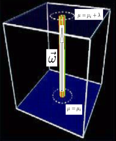
Figure 1: A thin tube surrounding a vortex line

the vorticity flux contained within the tube which is equal to the circulation around the tube is:

$$\Delta\Phi=\int\vec{\omega}\cdot d\vec{S}=\oint\vec{v}\cdot d\vec{r}$$ (20)

and the mass contained with the tube is:

$$\Delta M=\int\rho d\vec{l}\cdot d\vec{S}$$ (21)

in which $dl$ is a length element along the tube. Since the vortex lines move with the flow by virtue of equation (3) both the quantities $\Delta\Phi$ and $\Delta M$ are conserved and since the tube is thin we may define the conserved load:

$$\lambda=\frac{\Delta M}{\Delta\Phi}=\oint\frac{\rho}{\omega}dl$$ (22)

in which the above integral is performed along the field line. Obviously the parts of the line which go out of the flow to regions in which $\rho=0$ has a null contribution to the integral. Since $\lambda$ is conserved is satisfies the equation:

$$\frac{d\lambda}{dt}=0.$$ (23)

By construction surfaces of constant load move with the flow and contain vortex lines. Hence the gradient to such surfaces must be orthogonal to the field line:

$$\vec{\nabla}\lambda\cdot\vec{\omega}=0$$ (24)

Now consider an arbitrary comoving point on the vortex line and donate it by $i$, and consider an additional comoving point on the vortex line and donate it by $r$. The integral:

$$\mu(r)=\int_{i}^{r}\frac{\rho}{\omega}dl+\mu(i)$$ (25)

is also a conserved quantity which we may denote following Lynden-Bell & Katz [6] as the generalized metage. $\mu(i)$ is an arbitrary number which can be chosen differently for each vortex line. By construction:

$$\frac{d\mu}{dt}=0.$$ (26)

Also it is easy to see that by differentiating along the vortex line we obtain:

$$\vec{\nabla}\mu\cdot\vec{\omega}=\rho$$ (27)

At this point we have two comoving coordinates of flow, namely $\lambda,\mu$ obviously in a three dimensional flow we also have a third coordinate. However, before defining the third coordinate we will find it useful to work not directly with $\lambda$ but with a function of $\lambda$. Now consider the vortical flux $\Phi(\lambda)$ within a surface of constant load as described in figure 2

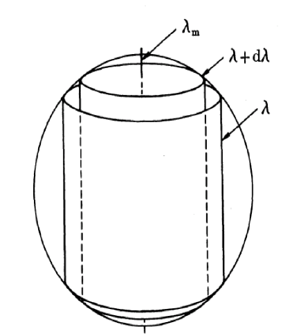
Figure 2: Surfaces of constant load

(the figure was given by Lynden-Bell & Katz [6]). The flux is a conserved quantity and depends only on the load $\lambda$ of the surrounding surface. Now we define the quantity:

$$\alpha=\frac{\Phi(\lambda)}{2\pi}=\frac{C(\lambda)}{2\pi}$$ (28)

$C(\lambda)$ is the circulation along lines on this surface. Obviously $\alpha$ satisfies the equations:

$$\frac{d\alpha}{dt}=0,\qquad\vec{\omega}\cdot\vec{\nabla}\alpha=0$$ (29)

Let us now define an additional comoving coordinate $\beta^{*}$ since $\vec{\nabla}\mu$ is not orthogonal to the $\vec{\omega}$ lines we can choose $\vec{\nabla}\beta^{*}$ to be orthogonal to the $\vec{\omega}$ lines and not be in the direction of the $\vec{\nabla}\alpha$ lines, that is we choose $\beta^{*}$ not to depend only on $\alpha$. Since both $\vec{\nabla}\beta^{*}$ and $\vec{\nabla}\alpha$ are orthogonal to $\vec{\omega}$, $\vec{\omega}$ must take the form:

$$\vec{\omega}=A\vec{\nabla}\alpha\times\vec{\nabla}\beta^{*}$$ (30)

However, using equation (4) we have:

$$\vec{\nabla}\cdot\vec{\omega}=\vec{\nabla}A\cdot(\vec{\nabla}\alpha\times\vec{\nabla}\beta^{*})=0$$ (31)

Which implies that $A$ is a function of $\alpha,\beta^{*}$. Now we can define a new comoving function $\beta$ such that:

$$\beta=\int_{0}^{\beta^{*}}A(\alpha,\beta^{{}^{\prime}*})d\beta^{{}^{\prime}*},\qquad\frac{d\beta}{dt}=0$$ (32)

In terms of this function we recover the representation given in equation (14):

$$\vec{\omega}=\vec{\nabla}\alpha\times\vec{\nabla}\beta$$ (33)

Hence we have shown how $\alpha,\beta$ can be constructed for a known $\vec{v},\rho$. Notice however, that $\beta$ is defined in a non unique way since one can redefine $\beta$ for example by performing the following transformation: $\beta\rightarrow\beta+f(\alpha)$ in which $f(\alpha)$ is an arbitrary function. The comoving coordinates $\alpha,\beta$ serve as labels of the vortex lines. Moreover the vortical flux can be calculated as:

$$\Phi=\int\vec{\omega}\cdot d\vec{S}=\int d\alpha d\beta$$ (34)

Finally we can use equation (8) to derive the function $\nu$ for any point $s$ within the flow:

$$\nu(s)=\int_{i}^{s}(\vec{v}-\alpha\vec{\nabla}\beta)\cdot d\vec{r}+\nu(i)$$ (35)

in which $i$ is any arbitrary point within the flow, the result will not depend on the trajectory taken in the case that $\nu$ is single valued. If $\nu$ is not single valued on should introduce a cut, which the integration trajectory should not cross.

2.4 Stationary fluid dynamics

Stationary flows are a unique phenomena of Eulerian fluid dynamics which has no counter part in Lagrangian fluid dynamics. The stationary flow is defined by the fact that the physical fields $\vec{v},\rho$ do not depend on the temporal coordinate. This however does not imply that the stationary potentials $\alpha,\beta,\nu$ are all functions of spatial coordinates alone. Moreover, it can be shown that choosing the potentials in such a way will lead to erroneous results in the sense that the stationary equations of motion can not be derived from the Lagrangian density $\hat{\cal L}$ given in equation (19). However, this problem can be amended easily as follows. Let us choose $\alpha,\nu$ to depend on the spatial coordinates alone. Let us choose $\beta$ such that:

$$\beta=\bar{\beta}-t$$ (36)

in which $\bar{\beta}$ is a function of the spatial coordinates. The Lagrangian density $\hat{\cal L}$ given in equation (19) will take the form:

$$\hat{\cal L}=\rho\left(\alpha-\varepsilon(\rho)-\frac{1}{2}(\vec{\nabla}\nu+\alpha\vec{\nabla}\beta)^{2}\right)$$ (37)

Varying the Lagrangian $\hat{L}=\int\hat{\cal L}d^{3}x$ with respect to $\alpha,\beta,\nu,\rho$ leads to the following equations:

$$\vec{\nabla}\cdot(\rho\hat{\vec{v}})=0$$

$$\rho\hat{\vec{v}}\cdot\vec{\nabla}\alpha=0$$

$$\rho(\hat{\vec{v}}\cdot\vec{\nabla}\bar{\beta}-1)=0$$

$$\alpha=\frac{1}{2}\hat{\vec{v}}^{2}+h$$ (38)

$\alpha$ is thus the Bernoulli constant (this was also noticed in [8]). Calculations similar to the ones done in previous subsections will show that those equations lead to the stationary Euler equations:

$$\rho(\hat{\vec{v}}\cdot\vec{\nabla})\hat{\vec{v}}=-\vec{\nabla}p(\rho)$$ (39)

3 A simpler variational principle of non-stationary fluid dynamics

Lynden-Bell & Katz [6] have shown that an Eulerian variational principle for non-stationary fluid dynamics can be given in terms of two functions the density $\rho$ and the non-magnetic load $\lambda$ defined in equation (22). However, their velocity was given an implicit definition in terms of a partial differential equation and its variations was constrained to satisfy this equation. In this section we will propose a three function variational principle in which the variations of the functions are not constrained in any way, part of our derivation will overlap the formalism of Lynden-Bell & Katz. The three variables will include the density $\rho$, the non-magnetic load $\lambda$ and an additional function to be defined in the next subsection. This variational principle is simpler than the Seliger & Whitham variational principle [5] which is given in terms of four functions and is more convenient than the Lynden-Bell & Katz [6] variational principle since the variations are not constrained.

3.1 Velocity representation

Consider equation (24), since $\vec{\omega}$ is orthogonal to $\vec{\nabla}\lambda$ we can write:

$$\vec{\omega}=\vec{K}\times\vec{\nabla}\lambda$$ (40)

in which $\vec{K}$ is some arbitrary vector field. However, since $\vec{\nabla}\cdot\vec{\omega}=0$ it follows that $\vec{K}=\vec{\nabla}\theta$ for some scalar function theta. Hence we can write:

$$\vec{\nabla}\times\vec{v}=\vec{\omega}=\vec{\nabla}\theta\times\vec{\nabla}\lambda$$ (41)

This will lead to:

$$\vec{v}=\theta\vec{\nabla}\lambda+\vec{\nabla}\nu$$ (42)

For the time being $\nu$ is an arbitrary scalar function, the choice of notation will be justified later. Consider now equation (23), inserting into this equation $\vec{v}$ given in equation (42) will result in:

$$\frac{d\lambda}{dt}=\frac{\partial\lambda}{\partial t}+\vec{v}\cdot\vec{\nabla}\lambda=\frac{\partial\lambda}{\partial t}+(\theta\vec{\nabla}\lambda+\vec{\nabla}\nu)\cdot\vec{\nabla}\lambda=0.$$ (43)

This can be solved for $\theta$, the solution obtained is:

$$\theta=-\left(\frac{\frac{\partial\lambda}{\partial t}+\vec{\nabla}\lambda\cdot\vec{\nabla}\nu}{|\vec{\nabla}\lambda|^{2}}\right)$$ (44)

Inserting the above expression for $\theta$ into equation (42) will yield:

$$\vec{v}=-\frac{\frac{\partial\lambda}{\partial t}}{|\vec{\nabla}\lambda|}\hat{\lambda}+\vec{\nabla}\nu-\hat{\lambda}(\hat{\lambda}\cdot\vec{\nabla}\nu)\equiv-\frac{\frac{\partial\lambda}{\partial t}}{|\vec{\nabla}\lambda|}\hat{\lambda}+\vec{\nabla}^{*}\nu$$ (45)

in which $\hat{\lambda}=\frac{\vec{\nabla}\lambda}{|\vec{\nabla}\lambda|}$ is a unit vector perpendicular to the load surfaces and $\vec{\nabla}^{*}\nu=\vec{\nabla}\nu-\hat{\lambda}(\hat{\lambda}\cdot\vec{\nabla}\nu)$ is the component of $\vec{\nabla}\nu$ parallel to the load surfaces. Notice that the vector $\vec{v}-\vec{\nabla}\nu$ is orthogonal to the load surfaces and that:

$$|\vec{v}-\vec{\nabla}\nu|=(\vec{v}-\vec{\nabla}\nu)\cdot\hat{\lambda}=\theta|\vec{\nabla}\lambda|\Rightarrow\theta=\frac{(\vec{v}-\vec{\nabla}\nu)\cdot\hat{\lambda}}{|\vec{\nabla}\lambda|}$$ (46)

Further more by construction the velocity field $\vec{v}$ given by equation (45) ensures that the load surfaces are comoving. Let us calculate the circulation along $\lambda$ surfaces:

$$C(\lambda)=\oint_{\lambda}\vec{v}\cdot d\vec{r}=\oint_{\lambda}\vec{\nabla}^{*}\nu\cdot d\vec{r}=\oint_{\lambda}\vec{\nabla}\nu\cdot d\vec{r}=[\nu]_{\lambda}$$ (47)

$[\nu]_{\lambda}$ is the discontinuity of $\nu$ across a cut which is introduced on the $\lambda$ surface. Hence in order that circulation $C(\lambda)$ on the load surfaces (and hence everywhere) will not vanish $\nu$ must be multiple-valued. Following Lamb [16, page 180, article 132, equation 1] we write $\nu$ in the form:

$$\nu=C(\lambda)\bar{\nu},\qquad[\bar{\nu}]_{\lambda}=1$$ (48)

in terms of $\bar{\nu}$ the velocity is given as:

$$\vec{v}=-\frac{\frac{\partial\lambda}{\partial t}}{|\vec{\nabla}\lambda|}\hat{\lambda}+C(\lambda)\vec{\nabla}^{*}\bar{\nu}$$ (49)

And the explicit dependence of the velocity field $\vec{v}$ on the circulation along the load surfaces $C(\lambda)$ is evident.

3.2 The variational principle

Consider the action:

$$A \equiv \int{\cal L}d^{3}xdt$$

$${\cal L} \equiv {\cal L}_{1}+{\cal L}_{2}$$

$${\cal L}_{1} \equiv \rho(\frac{1}{2}\vec{v}^{2}-\varepsilon(\rho)),\qquad{\cal L}_{2}\equiv\nu[\frac{\partial{\rho}}{\partial t}+\vec{\nabla}\cdot(\rho\vec{v})]$$ (50)

In which $\vec{v}$ is defined by equation (45). $\nu$ is not a simple Lagrange multiplier since $\vec{v}$ is dependent on $\nu$ through equation (45). Taking the variational derivative of ${\cal L}$ with respect to $\nu$ will yield:

$$\delta_{\nu}{\cal L}=\delta\nu[\frac{\partial{\rho}}{\partial t}+\vec{\nabla}\cdot(\rho\vec{v})]+\rho\vec{v}\cdot\delta_{\nu}\vec{v}+\nu\vec{\nabla}\cdot(\rho\delta_{\nu}\vec{v})$$ (51)

This can be rewritten as:

$$\delta_{\nu}{\cal L}=\delta\nu[\frac{\partial{\rho}}{\partial t}+\vec{\nabla}\cdot(\rho\vec{v})]+\rho(\vec{v}-\vec{\nabla}\nu)\cdot\delta_{\nu}\vec{v}+\vec{\nabla}\cdot(\rho\nu\delta_{\nu}\vec{v})$$ (52)

Now by virtue of equation (45):

$$\delta_{\nu}\vec{v}=\vec{\nabla}^{*}\delta\nu$$ (53)

which is parallel to the load surfaces, while from equation (42) we see that $\vec{v}-\vec{\nabla}\nu$ is orthogonal to the load surfaces. Hence, the scalar product of those vector must be null and we can write:

$$\delta_{\nu}{\cal L}=\delta\nu[\frac{\partial{\rho}}{\partial t}+\vec{\nabla}\cdot(\rho\vec{v})]+\vec{\nabla}\cdot(\rho\nu\vec{\nabla}^{*}\delta\nu)$$ (54)

Thus the action variation can be written as:

$$\delta_{\nu}A = \int d^{3}xdt\delta\nu[\frac{\partial{\rho}}{\partial t}+\vec{\nabla}\cdot(\rho\vec{v})]$$ (55)

$$+ \oint d\vec{S}\cdot\rho\nu\vec{\nabla}^{*}\delta\nu$$

This will yield the continuity equation using the standard variational procedure. Notice that the surface should include also the ”cut” since the $\nu$ function is in general multi valued. Let us now take the variational derivative with respect to the density $\rho$, we obtain:

$$\delta_{\rho}A = \int d^{3}xdt\delta\rho[\frac{1}{2}\vec{v}^{2}-w-\frac{\partial{\nu}}{\partial t}-\vec{v}\cdot\vec{\nabla}\nu]$$ (56)

$$+ \oint d\vec{S}\cdot\vec{v}\delta\rho\nu+\int d^{3}x\nu\delta\rho|^{t_{1}}_{t_{0}}$$

Hence provided that $\delta\rho$ vanishes on the boundary of the domain and in initial and final times the following equation must be satisfied:

$$\frac{d\nu}{dt}=\frac{1}{2}\vec{v}^{2}-w$$ (57)

This is the same equation as equation (10) and justifies the use of the symbol $\nu$ in equation (42). Finally we have to calculate the variation of the Lagrangian density with respect to $\lambda$ this will lead us to the following results:

$$\delta_{\lambda}{\cal L} = \rho\vec{v}\cdot\delta_{\lambda}\vec{v}+\nu\vec{\nabla}\cdot(\rho\delta_{\lambda}\vec{v})=\rho(\vec{v}-\vec{\nabla}\nu)\cdot\delta_{\lambda}\vec{v}+\vec{\nabla}\cdot(\rho\nu\delta_{\lambda}\vec{v})$$ (58)

$$= \rho\theta|\vec{\nabla}\lambda|(\hat{\lambda}\cdot\delta_{\lambda}\vec{v})+\vec{\nabla}\cdot(\rho\nu\delta_{\lambda}\vec{v})$$

in equation (46) was used. Let us calculate $\delta_{\lambda}\vec{v}$, after some straightforward manipulations one arrives at the result:

$$\delta_{\lambda}\vec{v}=-\frac{\hat{\lambda}}{|\vec{\nabla}\lambda|}\left[\frac{\partial(\delta\lambda)}{\partial t}+\vec{v}\cdot\vec{\nabla}\delta\lambda\right]+\theta\vec{\nabla}^{*}\delta\lambda$$ (59)

Inserting equation (59) into equation (58) and integrating by parts will yield:

$$\delta_{\lambda}{\cal L}=\delta\lambda\left[\frac{\partial(\rho\theta)}{\partial t}+\vec{\nabla}\cdot(\rho\theta\vec{v})\right]+\vec{\nabla}\cdot[\rho(\delta_{\lambda}\vec{v}\nu-\theta\vec{v}\delta\lambda)]-\frac{\partial(\rho\theta\delta\lambda)}{\partial t}$$ (60)

Hence the total variation of the action will become:

$$\delta_{\lambda}A = \int d^{3}xdt\delta\lambda\left[\frac{\partial(\rho\theta)}{\partial t}+\vec{\nabla}\cdot(\rho\theta\vec{v})\right]$$ (61)

$$+ \oint d\vec{S}\cdot(\delta_{\lambda}\vec{v}\nu-\theta\vec{v}\delta\lambda)\rho-\int d^{3}x\rho\theta\delta\lambda|^{t_{1}}_{t_{0}}$$

Hence choosing $\delta\lambda$ in such a way that the temporal and spatial boundary terms vanish in the above integral will lead to the equation:

$$\frac{\partial{(\rho\theta)}}{\partial t}+\vec{\nabla}\cdot(\rho\theta\vec{v})=0$$ (62)

Using the continuity equation (1) will lead to the equation:

$$\rho\frac{d\theta}{dt}=0$$ (63)

Hence for $\rho\neq 0$ both $\lambda$ and $\theta$ are comoving. Comparing equation (8) to equation (42) we see that $\alpha$ is analogue to $\theta$ and $\beta$ is analogue to $\lambda$ and all those variables are comoving. Furthermore, the $\nu$ function in equation (42) satisfies the same equation as the $\nu$ appearing in equation (8) which is equation (57). It follows immediately without the need for any additional calculations that $\vec{v}$ given in equation (42) satisfies Euler’s equations (2), the proof for this is given in subsection 2.1 in which one should replace $\alpha$ with $\theta$ and $\beta$ with $\lambda$. Thus all the equations of fluid dynamics can be derived from the action (50) without restricting the variations in any way. The reader should notice an important difference between the current and previous formalism. In the current formalism $\theta$ is a dependent variable defined by equation (44), while in the previous formalism the analogue quantity $\alpha$ was an independent variational variable. Thus equation (63) should be considered as some what complicated second-order partial differential equation (in the temporal coordinate $t$) for $\lambda$ which should be solved simultaneously with equation (57) and equation (1).

3.3 Simplified action

The Lagrangian density ${\cal L}$ given in equation (50) can be written explicitly in terms of the three variational variables $\rho,\lambda,\nu$ as follows:

$${\cal L} = \hat{\cal L}+{\cal L}_{boundary}$$

$$\hat{\cal L} \equiv \rho\left[\frac{1}{2}\left(\frac{\frac{\partial{\lambda}}{\partial t}+\vec{\nabla}\lambda\cdot\vec{\nabla}\nu}{|\vec{\nabla}\lambda|}\right)^{2}-\frac{1}{2}(\vec{\nabla}\nu)^{2}-\frac{\partial\nu}{\partial t}-\varepsilon(\rho)\right]$$

$${\cal L}_{boundary} \equiv \frac{\partial{(\nu\rho)}}{\partial t}+\vec{\nabla}\cdot(\nu\rho\vec{v})$$ (64)

Notice that the term ${\cal L}_{boundary}$ contains only complete partial derivatives and thus can not contribute to the equations although it can change the boundary conditions. Hence we see that equation (1), equation (57) and equation (63) can be derived using the Lagrangian density $\hat{\cal L}$ in which $\vec{v}$ is given in terms of equation (45) in the relevant equations. Furthermore, after integrating those three equations we can insert the potentials $\lambda,\nu$ into equation (45) to obtain the physical velocity $\vec{v}$. Hence, the general barotropic fluid dynamics problem is altered such that instead of solving the four equations (1,2) we need to solve an alternative set of three equations which can be derived from the Lagrangian density $\hat{\cal L}$. Notice that the specific choice of the labelling of the $\lambda$ surfaces is not important in the above Lagrangian density one can replace: $\lambda->\Lambda(\lambda)$, without changing the Lagrangian functional form. This means that only the shape of the $\lambda$ surface is important not their labelling. In group theoretic language this implies that the Lagrangian is invariant under an infinite symmetry group and hence should posses an infinite number of constants of motion. In terms of the Lamb type function $\bar{\nu}$ defined in equation (48), the Lagrangian density given in equation (50) can be rewritten in the form:

$${\cal L} = \hat{\cal L}+{\cal L}_{boundary}$$

$$\hat{\cal L} \equiv \rho\left[\frac{1}{2}\left(\frac{\frac{\partial{\lambda}}{\partial t}+C(\lambda)\vec{\nabla}\lambda\cdot\vec{\nabla}\bar{\nu}}{|\vec{\nabla}\lambda|}\right)^{2}-\frac{1}{2}(C(\lambda)\vec{\nabla}\bar{\nu})^{2}-C(\lambda)\frac{\partial\bar{\nu}}{\partial t}-\varepsilon(\rho)\right]$$

$${\cal L}_{boundary} \equiv \frac{\partial{(C(\lambda)\bar{\nu}\rho)}}{\partial t}+\vec{\nabla}\cdot(C(\lambda)\bar{\nu}\rho\vec{v})$$ (65)

Which emphasize the dependence of the Lagrangian on the the circulations along the load surfaces $C(\lambda)$ which are given as initial conditions.

3.4 Stationary fluid dynamics

For stationary flows we assume that both the density $\rho$ and the load $\lambda$ are time independent. Hence the velocity field given in equation (45) can be written as:

$$\vec{v}=\vec{\nabla}\nu-\hat{\lambda}(\hat{\lambda}\cdot\vec{\nabla}\nu)=\vec{\nabla}^{*}\nu=C(\lambda)\vec{\nabla}^{*}\bar{\nu}$$ (66)

thus the stationary flow is parallel to the load surfaces. From the above equation we see that in the stationary case $\nu$ can be written in the form:

$$\nu=\nu_{0}-f(\lambda,t)$$ (67)

in which $f(\lambda,t)$ is an arbitrary function and $\nu_{0}$ is independent of the temporal coordinate. Hence we can rewrite the velocity $\vec{v}$ as:

$$\vec{v}=\vec{\nabla}^{*}\nu_{0}=C(\lambda)\vec{\nabla}^{*}\bar{\nu}_{0}$$ (68)

Inserting equation (67) and equation (68) into equation (57) will yield:

$$\frac{\partial f(\lambda,t)}{\partial t}=\frac{1}{2}\vec{v}^{2}+w=B(\lambda)$$ (69)

in which $B(\lambda)$ is the Bernoulli constant. Integrating we obtain:

$$f(\lambda,t)=B(\lambda)t+g(\lambda)$$ (70)

the arbitrary $g(\lambda)$ function can be absorbed into $\nu_{0}$ and thus we rewrite equation (67) in the form:

$$\nu=\nu_{0}-B(\lambda)t$$ (71)

Further more we can rewrite the conserved quantity $\theta$ given in equation (44) as:

$$\theta=-\left(\frac{\vec{\nabla}\lambda\cdot\vec{\nabla}\nu}{|\vec{\nabla}\lambda|^{2}}\right)=-\left(\frac{\hat{\lambda}\cdot\vec{\nabla}\nu_{0}}{|\vec{\nabla}\lambda|}\right)+t\frac{dB(\lambda)}{d\lambda}$$ (72)

The Lagrangian density ${\cal L}$ given in equation (50) can be written in the stationary case taking into account equation (68) and equation (71) as follows:

$$\hat{\cal L} = \rho\left[\frac{1}{2}(\hat{\lambda}\cdot\vec{\nabla}\nu)^{2}-\frac{1}{2}(\vec{\nabla}\nu)^{2}+B(\lambda)-\varepsilon(\rho)\right]$$ (73)

$$= \rho\left[B(\lambda)-\frac{1}{2}(\vec{\nabla}^{*}\nu_{0})^{2}-\varepsilon(\rho)\right]$$

$$= \rho\left[B(\lambda)-\frac{1}{2}(C(\lambda)\vec{\nabla}^{*}\bar{\nu}_{0})^{2}-\varepsilon(\rho)\right]$$

Taking the variational derivative of the Lagrangian density $\hat{\cal L}$ with respect to the mass density $\rho$ will yield the Bernoulli equation (69). The variation of the Lagrangian $\hat{L}=\int d^{3}x\hat{\cal L}$ with respect to $\nu_{0}$ will yield the mass conservation equation:

$$\vec{\nabla}^{*}\cdot(\rho\vec{v})=0$$ (74)

this form is equivalent to the standard stationary continuity equation
$\vec{\nabla}\cdot(\rho\vec{v})=0$ since there is no mass flux orthogonal to the load surfaces. Finally taking the variation of $\hat{L}$ with respect to $\lambda$ will yield:

$$\rho\left[\frac{dB}{d\lambda}-\vec{v}\cdot\vec{\nabla}^{*}\left(\frac{\hat{\lambda}\cdot\vec{\nabla}\nu_{0}}{|\vec{\nabla}\lambda|}\right)\right]=0$$ (75)

Which can be also obtained by inserting equation (72) into equation (63). Hence we obtained three equations (69,74,75) for the three spatial functions $\rho,\lambda$ and $\nu_{0}$. Admittedly those equations do not have a particularly simple form, we will obtain a somewhat better set of equations in the next section.

4 Simplified variational principle for stationary fluid dynamics

In the previous sections we have shown that fluid dynamics can be described in terms of four first order differential equations and in term of an action principle from which those equations can be derived. An alternative derivation in terms of three differential equations one of which (equation (63)) is second order has been introduced as well. Those formalisms were shown to apply to both stationary and non-stationary fluid dynamics. In the following a different three functions formalism for stationary fluid dynamics is introduced. In the suggested representation, the Euler and continuity equations can be integrated leaving only an algebraic equation to solve.

Consider equation (13), for a stationary flow it takes the form:

$$\vec{v}\cdot\vec{\nabla}\alpha=0$$ (76)

Hence $\vec{v}$ can take the form:

$$\vec{v}=\frac{\vec{\nabla}\alpha\times\vec{K}}{\rho}$$ (77)

However, since the velocity field must satisfy the stationary mass conservation equation equation (1):

$$\vec{\nabla}\cdot(\rho\vec{v})=0$$ (78)

We see that $\vec{K}$ must have the form $\vec{K}=\vec{\nabla}N$, where $N$ is an arbitrary function. Thus, $\vec{v}$ takes the form:

$$\vec{v}=\frac{\vec{\nabla}\alpha\times\vec{\nabla}N}{\rho}$$ (79)

Let us now calculate $\vec{v}\times\vec{\omega}$ in which $\vec{\omega}$ is given by equation (14), hence:

$$\vec{v}\times\vec{\omega} = (\frac{\vec{\nabla}\alpha\times\vec{\nabla}N}{\rho})\times(\vec{\nabla}\alpha\times\vec{\nabla}\beta)$$ (80)

$$= \frac{1}{\rho}\vec{\nabla}\alpha(\vec{\nabla}\alpha\times\vec{\nabla}N)\cdot\vec{\nabla}\beta$$

Now since the flow is stationary $N$ can be at most a function of the three comoving coordinates $\alpha,\bar{\beta},\mu$ defined in subsections 2.2 and 2.4, hence:

$$\vec{\nabla}N=\frac{\partial N}{\partial\alpha}\vec{\nabla}\alpha+\frac{\partial N}{\partial\bar{\beta}}\vec{\nabla}\bar{\beta}+\frac{\partial N}{\partial\mu}\vec{\nabla}\mu$$ (81)

Inserting equation (81) into equation (80) will yield:

$$\vec{v}\times\vec{\omega}=\frac{1}{\rho}\vec{\nabla}\alpha\frac{\partial N}{\partial\mu}(\vec{\nabla}\alpha\times\vec{\nabla}\mu)\cdot\vec{\nabla}\bar{\beta}$$ (82)

Rearranging terms and using vorticity formula (14) we can simplify the above equation and obtain:

$$\vec{v}\times\vec{\omega}=-\frac{1}{\rho}\vec{\nabla}\alpha\frac{\partial N}{\partial\mu}(\vec{\nabla}\mu\cdot\vec{\omega})$$ (83)

However, using equation (27) this will simplify to the form:

$$\vec{v}\times\vec{\omega}=-\vec{\nabla}\alpha\frac{\partial N}{\partial\mu}$$ (84)

Now let us consider equation (3), for stationary flows this will take the form:

$$\vec{\nabla}\times(\vec{v}\times\vec{\omega})=0$$ (85)

Inserting equation (84) into equation (85) will lead to the equation:

$$\vec{\nabla}(\frac{\partial N}{\partial\mu})\times\vec{\nabla}\alpha=0$$ (86)

However, since $N$ is at most a function of $\alpha,\bar{\beta},\mu$. It follows that $\frac{\partial N}{\partial\mu}$ is some function of $\alpha$:

$$\frac{\partial N}{\partial\mu}=-F(\alpha)$$ (87)

This can be easily integrated to yield:

$$N=-\mu F(\alpha)+G(\alpha,\bar{\beta})$$ (88)

Inserting this back into equation (79) will yield:

$$\vec{v}=\frac{\vec{\nabla}\alpha\times(-F(\alpha)\vec{\nabla}\mu+\frac{\partial G}{\partial{\bar{\beta}}}\vec{\nabla}\bar{\beta})}{\rho}$$ (89)

Let us now replace the set of variables $\alpha,\bar{\beta}$ with a new set $\alpha^{\prime},\bar{\beta}^{\prime}$ such that:

$$\alpha^{\prime}=\int F(\alpha)d\alpha,\qquad\bar{\beta}^{\prime}=\frac{\bar{\beta}}{F(\alpha)}$$ (90)

This will not have any effect on the vorticity presentation given in equation (14) since:

$$\vec{\omega}=\vec{\nabla}\alpha\times\vec{\nabla}\beta=\vec{\nabla}\alpha\times\vec{\nabla}\bar{\beta}=\vec{\nabla}\alpha^{\prime}\times\vec{\nabla}\bar{\beta}^{\prime}$$ (91)

However, the velocity will have a simpler presentation and will take the form:

$$\vec{v}=\frac{\vec{\nabla}\alpha^{\prime}\times\vec{\nabla}(-\mu+G^{\prime}(\alpha^{\prime},\bar{\beta}^{\prime}))}{\rho}$$ (92)

in which $G^{\prime}=\frac{G}{F}$. At this point one should remember that $\mu$ was defined in equation (25) up to an arbitrary constant which can very between vortex lines. Since the lines are labelled by their $\alpha^{\prime},\bar{\beta}^{\prime}$ values it follows that we can add an arbitrary function of $\alpha^{\prime},\bar{\beta}^{\prime}$ to $\mu$ without effecting its properties. Hence we can define a new $\mu^{\prime}$ such that:

$$\mu^{\prime}=\mu-G^{\prime}(\alpha^{\prime},\bar{\beta}^{\prime})$$ (93)

Inserting equation (93) into equation (92) will lead to a simplified equation for $\vec{v}$:

$$\vec{v}=\frac{\vec{\nabla}\mu^{\prime}\times\vec{\nabla}\alpha^{\prime}}{\rho}$$ (94)

In the following the primes on $\alpha,\bar{\beta},\mu$ will be ignored. It is obvious that $\vec{v}$ satisfies the following set of equations:

$$\vec{v}\cdot\vec{\nabla}\mu=0,\qquad\vec{v}\cdot\vec{\nabla}\alpha=0,\qquad\vec{v}\cdot\vec{\nabla}\bar{\beta}=1$$ (95)

to derive the right hand equation we have used both equation (27) and equation (14). Hence $\mu,\alpha$ are both comoving and stationary. As for $\bar{\beta}$ it satisfies equation (38).

By vector multiplying $\vec{v}$ and $\vec{\omega}$ and using equations (94,14) we obtain:

$$\vec{v}\times\vec{\omega}=\vec{\nabla}\alpha$$ (96)

this means that both $\vec{v}$ and $\vec{\omega}$ lie on $\alpha$ surfaces and provide a vector basis for this two dimensional surface.

4.1 The action principle

In the previous subsection we have shown that if the velocity field $\vec{v}$ is given by equation (94) than equation (1) is satisfied automatically for stationary flows. To complete the set of equations we will show how the Euler equations (2) can be derived from the Lagrangian:

$$L \equiv \int{\cal L}d^{3}x$$

$${\cal L} \equiv \rho(\frac{1}{2}\vec{v}^{2}-\varepsilon(\rho))$$ (97)

In which $\vec{v}$ is given by equation (94) and the density $\rho$ is given by equation (27):

$$\rho=\vec{\nabla}\mu\cdot\vec{\omega}=\vec{\nabla}\mu\cdot(\vec{\nabla}\alpha\times\vec{\nabla}\beta)=\frac{\partial(\alpha,\beta,\mu)}{\partial(x,y,z)}$$ (98)

In this case the Lagrangian density of equation (97) will take the form:

$${\cal L}=\rho\left(\frac{1}{2}(\frac{\vec{\nabla}\mu\times\vec{\nabla}\alpha}{\rho})^{2}-\varepsilon(\rho)\right)$$ (99)

and can be seen explicitly to depend on only three functions. The variational derivative of $L$ given in equation (97) is:

$$\delta L = \int\delta{\cal L}d^{3}x$$

$$\delta{\cal L} = \delta\rho(\vec{v}^{2}-w(\rho))+\rho\vec{v}\cdot\delta\vec{v}$$ (100)

Let us make arbitrary small variations $\delta\alpha_{i}=(\delta\alpha,\delta\beta,\delta\mu)$ of the functions $\alpha_{i}=(\alpha,\beta,\mu)$. Let us define the vector:

$$\vec{\xi}\equiv-\frac{\partial\vec{r}}{\partial\alpha_{i}}\delta\alpha_{i}$$ (101)

This will lead to the equation:

$$\delta\alpha_{i}=-\vec{\nabla}\alpha_{i}\cdot\vec{\xi}$$ (102)

Making a variation of $\rho$ given in equation (98) with respect to $\alpha_{i}$ will yield:

$$\delta\rho=-\vec{\nabla}\cdot(\rho\vec{\xi})$$ (103)

(for a proof see for example [13]). Calculating $\delta\vec{v}$ by varying equation (94) will give:

$$\delta\vec{v}=-\frac{\delta\rho}{\rho}\vec{v}+\frac{1}{\rho}\vec{\nabla}\times(\rho\vec{\xi}\times\vec{v})$$ (104)

Inserting equations (103,104) into equation (100) will yield:

$$\delta{\cal L} = \vec{v}\cdot\vec{\nabla}\times(\rho\vec{\xi}\times\vec{v})-\delta\rho(\frac{1}{2}\vec{v}^{2}+w)$$ (105)

$$= \vec{v}\cdot\vec{\nabla}\times(\rho\vec{\xi}\times\vec{v})+\vec{\nabla}\cdot(\rho\vec{\xi})(\frac{1}{2}\vec{v}^{2}+w)$$

Using the well known vector identity:

$$\vec{A}\cdot\vec{\nabla}\times(\vec{C}\times\vec{A})=\vec{\nabla}\cdot((\vec{C}\times\vec{A})\times\vec{A})+(\vec{C}\times\vec{A})\cdot\vec{\nabla}\times\vec{A}$$ (106)

and the theorem of Gauss we can write now equation (100) in the form:

$$\delta L = \oint d\vec{S}\cdot[(\vec{\xi}\times\vec{v})\times\vec{v}+(\frac{1}{2}\vec{v}^{2}+w)\vec{\xi}]\rho$$ (107)

$$+ \int d^{3}x\vec{\xi}\cdot[\vec{v}\times\vec{\omega}-\vec{\nabla}(\frac{1}{2}\vec{v}^{2}+w)]\rho$$

Suppose now that $\delta L=0$ for a $\vec{\xi}$ such that the boundary term in the above equation is null but that $\vec{\xi}$ is otherwise arbitrary, then it entails the equation:

$$\rho\vec{v}\times\vec{\omega}-\rho\vec{\nabla}(\frac{1}{2}\vec{v}^{2}+w)=0$$ (108)

Using the vector identity :

$$\frac{1}{2}\vec{\nabla}(\vec{v}^{2})=(\vec{v}\cdot\vec{\nabla})\vec{v}+\vec{v}\times(\vec{\nabla}\times\vec{v})$$ (109)

and rearranging terms we recover the stationary Euler equations:

$$\rho(\vec{v}\cdot\vec{\nabla})\vec{v}=-\vec{\nabla}p$$ (110)

4.2 The integration of the stationary Euler equations

Let us now combine equation (108) with equation (96), this will yield:

$$\vec{\nabla}\alpha=\vec{\nabla}(\frac{1}{2}\vec{v}^{2}+w)$$ (111)

which can easily be integrated to yield:

$$\alpha=\frac{1}{2}\vec{v}^{2}+w(\rho)$$ (112)

in which an arbitrary constant is absorbed into $\alpha$, this is consistent with equation (38) and implies that $\alpha$ is the Bernoulli constant. Let us now insert $\vec{v}$ given by equation (94) into the above equation:

$$\alpha=\frac{1}{2}\left(\frac{\vec{\nabla}\mu\times\vec{\nabla}\alpha}{\rho}\right)^{2}+w(\rho)$$ (113)

This can be rewritten as:

$$w(\rho)\rho^{2}-\rho^{2}\alpha+\frac{1}{2}(\vec{\nabla}\mu\times\vec{\nabla}\alpha)^{2}=0$$ (114)

By defining:

$$\Pi \equiv \rho^{2}$$

$$W(\Pi) \equiv w(\rho)$$ (115)

We obtain:

$$W(\Pi)\Pi-\Pi\alpha+\frac{1}{2}(\vec{\nabla}\mu\times\vec{\nabla}\alpha)^{2}=0$$ (116)

If one chooses an $\alpha$ and $\mu$ functions such that the above nonlinear equation has a positive (or zero) solution for $\Pi$ at every point in space than one obtains a solution of both the Euler and continuity equations in which $\vec{v}$ is given by equation (94) and $\rho=+\sqrt{\Pi}$. One should notice, however, that $\alpha$ and $\mu$ are not arbitrary functions. $\alpha$ is a function of the load defined in equation (22) and thus according to equation (24) must satisfy the equation:

$$\vec{\nabla}\alpha\cdot\vec{\omega}=0$$ (117)

that is both the velocity and vorticity fields must lie on the alpha surfaces. While for the velocity $\vec{v}$ this is assured by equation (94) this is not assured for the vorticity. Furthermore, $\mu$ is not an arbitrary function it is a metage function an thus must satisfy equation (27). Moreover, obtaining a solution does not imply that the obtained solution is stable. Having said that we notice that the technique requires only the solution of the algebraic equation (116) and does involve solving any differential equations.

5 Conclusion

In this paper we have reviewed Eulerian variational principles for non-stationary barotropic fluid dynamics and introduced a simpler three independent functions variational formalisms for stationary and non-stationary barotropic flows. This is less than the four variables which appear in the standard equations of fluid dynamics which are the velocity field $\vec{v}$ and the density $\rho$. We have shown how in terms of our new variables the stationary Euler and continuity equations can be integrated, such that the stationary Eulerian fluid dynamics problem is reduced to a non-linear algebraic equation for the density.

The problem of stability analysis and the description of numerical schemes using the described variational principles exceed the scope of this paper. We suspect that for achieving this we will need to add additional constants of motion constraints to the action as was done by [17, 18] see also [19], hopefully this will be discussed in a future paper.

References

- [1] 9
- [2] J. W. Herivel Proc. Camb. Phil. Soc., 51, 344 (1955)
- [3] J. Serrin, ‘Mathematical Principles of Classical Fluid Mechanics’ in Handbuch der Physik, 8, 148 (1959)
- [4] C. C. Lin , ‘Liquid Helium’ in Proc. Int. School Phys. XXI (Academic Press) (1963)
- [5] R. L. Seliger & G. B. Whitham, Proc. Roy. Soc. London, A305, 1 (1968)
- [6] D. Lynden-Bell and J. Katz ”Isocirculational Flows and their Lagrangian and Energy principles”, Proceedings of the Royal Society of London. Series A, Mathematical and Physical Sciences, Vol. 378, No. 1773, 179-205 (Oct. 8, 1981).
- [7] J. Katz & D. Lynden-Bell 1982,Proc. R. Soc. Lond. A 381 263-274.
- [8] A. Yahalom, ”Method and System for Numerical Simulation of Fluid Flow”, US patent 6,516,292 (2003).
- [9] A. Yahalom, & G. A. Pinhasi, ”Simulating Fluid Dynamics using a Variational Principle”, proceedings of the AIAA Conference, Reno, USA (2003).
- [10] A. Yahalom, G. A. Pinhasi and M. Kopylenko, ”A Numerical Model Based on Variational Principle for Airfoil and Wing Aerodynamics”, proceedings of the AIAA Conference, Reno, USA (2005).
- [11] D. Ophir, A. Yahalom, G. A. Pinhasi and M. Kopylenko ”A Combined Variational & Multi-grid Approach for Fluid Simulation” Proceedings of International Conference on Adaptive Modelling and Simulation (ADMOS 2005), pages 295-304, Barcelona, Spain (8-10 September 2005).
- [12] D. Lynden-Bell 1996, Current Science 70 No 9. 789-799.
- [13] J. Katz, S. Inagaki, and A. Yahalom, ”Energy Principles for Self-Gravitating Barotropic Flows: I. General Theory”, Pub. Astro. Soc. Japan 45, 421-430 (1993).
- [14] A. Yahalom ”Energy Principles for Barotropic Flows with Applications to Gaseous Disks” Thesis submitted as part of the requirements for the degree of Doctor of Philosophy to the Senate of the Hebrew University of Jerusalem (December 1996).
- [15] C. Eckart 1960 The Physics of Fluids, 3, 421.
- [16] H. Lamb Hydrodynamics Dover Publications (1945).
- [17] V. I. Arnold ”A variational principle for three-dimensional steady flows of an ideal fluid”, Appl. Math. Mech. 29, 5, 154-163.
- [18] V. I. Arnold ”On the conditions of nonlinear stability of planar curvilinear flows of an ideal fluid”, Dokl. Acad. Nauk SSSR 162 no. 5.
- [19] Yahalom A., Katz J. & Inagaki K. 1994, Mon. Not. R. Astron. Soc. 268 506-516.