Inversion formula of multifractal energy dissipation in 3D fully developed turbulence

Abstract

The concept of inverse statistics in turbulence has attracted much attention in the recent years. It is argued that the scaling exponents of the direct structure functions and the inverse structure functions satisfy an inversion formula. This proposition has already been verified by numerical data using the shell model. However, no direct evidence was reported for experimental three dimensional turbulence. We propose to test the inversion formula using experimental data of three dimensional fully developed turbulence by considering the energy dissipation rates in stead of the usual efforts on the structure functions. The moments of the exit distances are shown to exhibit nice multifractality. The inversion formula between the direct and inverse exponents is then verified.

Intermittency of fully developed isotropic turbulence is well captured by highly nontrivial scaling laws in structure functions and multifractal nature of energy dissipation rates Frisch (1996). The direct (longitudinal) structure function of order $q$ is defined by $S_{q}({r})\equiv\langle\Delta{v}_{\parallel}({r})^{q}\rangle$, where $\Delta{v}_{\parallel}({r})$ is the longitudinal velocity difference of two positions with a separation of $r$. The anomalous scaling properties characterized by $S_{q}({r})\sim r^{\zeta(q)}$ with a nonlinear scaling exponent function $\zeta(q)$ were uncovered experimentally Anselmet et al. (1984).

While the direct structure functions consider the statistical moments of the velocity increments $\Delta{v}$ measured over a distance $r$, the inverse structure functions are concerned with the exit distance $r$ where the velocity fluctuation exceeds the threshold $\Delta{v}$ at minimal distance Jensen (1999). An alternative quantity is thus introduced, denoted the distance structure functions Jensen (1999) or inverse structure functions Biferale et al. (1999, 2001), that is, $T_{q}(\Delta v)\equiv\langle{{r}^{q}(\Delta v)}\rangle$. Due to the duality between the two methodologies, one can intuitively expected that there is a power-law scaling stating that $T_{p}({\Delta{v}})\sim{\Delta{v}}^{\phi(p)}$, where $\phi(p)$ is a nonlinear concave function. This point is verified by the synthetic data from the GOY shell model of turbulence exhibiting perfect scaling dependence of the inverse structure functions on the velocity threshold Jensen (1999). Although the inverse structure functions of two-dimensional turbulence exhibit sound multifractal nature Biferale et al. (2001), a completely different result was obtained for three-dimensional turbulence, where an experimental signal at high Reynolds number was analyzed and no clear power law scaling was found in the exit distance structure functions Biferale et al. (1999). Instead, different experiments show that the inverse structure functions of three-dimensional turbulence exhibit clear extended self-similarity Beaulac and Mydlarski (2004); Pearson and van de Water (2005); Zhou et al. (2005).

For the classical binomial measures, Roux and Jensen Roux and Jensen (2004) have proved an exact relation between the direct and inverse scaling exponents,

$$\left\{\begin{array}[]{lll}\zeta(q)&=&-p\\ \phi(p)&=&-q\end{array}\right.~{},$$ (1)

which is verified by the simulated velocity fluctuations from the shell model. This same relation is also derived intuitively in an alternative way for velocity fields Schmitt (2005). A similar derivation was given for Laplace random walks as well Hastings (2002). However, this prediction (1) is not confirmed by wind-tunnel turbulence experiments (Reynolds numbers ${\mbox{Re}}=400-1100$) Pearson and van de Water (2005). We argue that this dilemma comes from the ignoring of the fact that velocity fluctuation is not a conservative measure like the binomial measure. In other words, Eq. (1) can not be applied to nonconservative multifractal measures.

Actually, Eq. (1) is known as the inversion formula and has been proved mathematically for both discontinuous and continuous multifractal measures Mandelbrot and Riedi (1997); Riedi and Mandelbrot (1997). Let $\mu$ be a probability measure on $[0,1]$ with its integral function $M(t)=\mu([0,t])$. Then its inverse measure can be defined by

$$\mu^{\dagger}=M^{\dagger}(s)=\left\{\begin{array}[]{lll}\inf\{t:M(t)>s\},&&{\mbox{if }}s<1\\ 1,&&{\mbox{if }}s=1\end{array}\right.~{},$$ (2)

where $M^{\dagger}(s)$ is the inverse function of $M(t)$. If $\mu$ is self-similar, then the relation $\mu=\sum_{i=1}^{n}p_{i}\mu(m_{i}^{-1}(\cdot))$ holds, where $m_{i}$’s are similarity maps with scale contraction ratios $r_{i}\in(0,1)$ and $\sum_{i=1}^{n}p_{i}=1$ with $p_{i}>0$. The multifractal spectrum of measure $\mu$ is the Legendre transform $f(\alpha)$ of $\tau$, which is defined by

$$\sum_{i=1}^{n}p_{i}^{q}r_{i}^{-\tau}=1~{}.$$ (3)

It can be shown that Mandelbrot and Riedi (1997); Riedi and Mandelbrot (1997), the inverse measure $\mu^{\dagger}$ is also self-similar with ratio $r_{i}^{\dagger}=p_{i}$ and $p_{i}^{\dagger}=r_{i}$, whose multifractal spectrum $f^{\dagger}(\alpha^{\dagger})$ is the Legendre transform of $\theta$, which is defined implicitly by

$$\sum_{i=1}^{n}(p_{i}^{\dagger})^{p}(r_{i}^{\dagger})^{-\theta}=1~{}.$$ (4)

It is easy to verify that the inversion formula holds that

$$\left\{\begin{array}[]{lll}\tau(q)&=&-p\\ \theta(p)&=&-q\end{array}\right.~{}.$$ (5)

Two equivalent testable formulae follow immediately that

$$\tau(q)=-\theta^{-1}(-q)$$ (6)

and

$$\theta(p)=-\tau^{-1}(-p)~{}.$$ (7)

Due to the conservation nature of the measure and its inverse in the formulation outlined above, we figure that it is better to test the inverse formula in turbulence by considering the energy dissipation.

Very good quality high-Reynolds turbulence data have been collected at the S1 ONERA wind tunnel by the Grenoble group from LEGI Anselmet et al. (1984). We use the longitudinal velocity data obtained from this group. The size of the velocity time series that we analyzed is $N\approx 1.73\times 10^{7}$.

The mean velocity of the flow is approximately $\langle{v}\rangle=20$m/s (compressive effects are thus negligible). The root-mean-square velocity fluctuations is $v_{\mathtt{rms}}=1.7$m/s, leading to a turbulence intensity equal to $I={v_{\mathtt{rms}}}/{\langle{v}\rangle}=0.0826$. This is sufficiently small to allow for the use of Taylor’s frozen flow hypothesis. The integral scale is approximately $4\mathtt{m}$ but is difficult to estimate precisely as the turbulent flow is neither isotropic nor homogeneous at these large scales.

The Kolmogorov microscale $\eta$ is given by Meneveau and Sreenivasan (1991) $\eta=\left[\frac{\nu^{2}\langle{v}\rangle^{2}}{15\langle(\partial v/\partial t)^{2}\rangle}\right]^{1/4}=0.195\mathtt{mm}$, where $\nu=1.5\times 10^{-5}\mathtt{m^{2}s^{-1}}$ is the kinematic viscosity of air. $\partial v/\partial t$ is evaluated by its discrete approximation with a time step increment $\partial t=3.5466\times 10^{-5}\mathtt{s}$ corresponding to the spatial resolution $\epsilon=0.72\mathtt{mm}$ divided by $\langle{v}\rangle$, which is used to transform the data from time to space applying Taylor’s frozen flow hypothesis.

The Taylor scale is given by Meneveau and Sreenivasan (1991) $\lambda=\frac{\langle{v}\rangle v_{\mathtt{rms}}}{\langle(\partial v/\partial t)^{2}\rangle^{1/2}}=16.6\mathtt{mm}$. The Taylor scale is thus about $85$ times the Kolmogorov scale. The Taylor-scale Reynolds number is $Re_{\lambda}=\frac{v_{\mathtt{rms}}\lambda}{\nu}=2000$. This number is actually not constant along the whole data set and fluctuates by about $20\%$.

We have checked that the standard scaling laws previously reported in the literature are recovered with this time series. In particular, we have verified the validity of the power-law scaling $E(k)\sim k^{-\beta}$ with an exponent $\beta$ very close to $\frac{5}{3}$ over a range more than two decades, similar to Fig. 5.4 of Frisch (1996) provided by Gagne and Marchand on a similar data set from the same experimental group. Similarly, we have checked carefully the determination of the inertial range by combining the scaling ranges of several velocity structure functions (see Fig. 8.6 of (Frisch, 1996, Fig. 8.6)). Conservatively, we are led to a well-defined inertial range $60\leq{r}/\eta\leq 2000$.

The exit distance sequence $r(\delta{E})=\{r_{j}(\delta{E})\}$ for a given energy threshold $\delta E$ can be obtained as follows. For a velocity time series $\{v_{i}=v(t_{i}):i=1,2,\cdots\}$, the energy dissipation rate series is constructed as $\{E_{i}=(v_{i+1}-v_{i})^{2}\}$. We assume that $E_{i}$ is distributed uniformly on the interval $[t_{i},t_{i+1})$. A right continuous energy density function is constructed such that $e(t)=E_{i}~{}{\rm{for}}~{}t\in[t_{i},t_{i+1})$. The exit distance sequence $\{r_{j}(\delta{E})\}$ is determined successively by $\sum_{k=1}^{j}{r_{k}}/{\langle{v}\rangle}=\inf\{t:\int_{0}^{t}e(t)dt\geqslant j\cdot\delta{E}\}$. Since energy is conservative, we have

$$r_{j}(2\delta{E})=r_{2j-1}(\delta{E})+r_{2j}(\delta{E})~{}.$$ (8)

With this relation, we can reduce the computational time significantly. In order to determine $r_{i}(\delta{E})$, we choose a minimal threshold $E_{\min}$, one tenth of the mean of $\{E_{i}\}$, and obtain $r_{i}(E_{\min})$. Then other sequences of $r_{i}$ for integer $\delta{E}/E_{\min}$ can be easily determined with relation (8).

In Fig. 1 is shown the empirical probability density functions (pdf’s) of exit distance $r/\eta$ for energy increments $E_{\min}$, $2E_{\min}$, and $4E_{\min}$. At a fist glance, the probability density functions are roughly Gaussian, as shown by the continuous curves in Fig. 1. The value of $\mu_{0}$ is the fitted parameter of the mean $\mu$ in the Gaussian distribution. For $r/\eta<\mu_{0}$, the three empirical pdf’s collapse to a single curve. However, for large $r/\eta>\mu_{0}$, the three empirical pdf’s differ from each other, especially in the right-hand-side tail distributions. This discrepancy is the cause of the occurrence of multifractal behavior of exit distance, which we shall show below.

An intriguing feature in the empirical pdf is emergence of small peaks observed at $r/\epsilon=1,2,\cdots$ in the tail distributions. Comparably, the pdf of exit distance of multinomial measure exhibits clear singular peaks. Therefore, these small peaks in Fig. 1 can be interpreted as finite-size truncations of singular distributions, showing the underlying singularity of the dissipation energy, which is consistent with the multifractal nature of the exit distance of dissipation energy.

According to the empirical probability density functions, the moments of exit distance exist for both positive and negative orders. Figure 2 illustrates the double logarithmic plots of $[T_{p}(r/\sum{r})]^{1/(p-1)}$ versus $\delta{E}/E$ for different values of $p$. For all values of $p$, the power-law dependence is evident. The straight lines are best fits to the data, whose slopes are estimates of $\theta(p)/(p-1)$.

The inverse scaling exponent $\theta(p)$ is plotted as triangles in Fig. 3 against order $p$, while the direct scaling exponent $\tau(q)$ is shown as open circles. We can obtain the function $-\tau^{-1}(-p)$ numerically from the $\tau(q)$ curve, which is shown as a dashed line. One can observe that the two functions $\theta(p)$ and $-\tau^{-1}(-p)$ coincide remarkably, which verifies the inverse formulation (6). Similarly, we obtained $-\theta^{-1}(-q)$ numerically from the $\theta(p)$ curve, shown as a solid line. Again, a nice agreements between $\tau(q)$ and $-\theta^{-1}(-q)$ is observed, which verifies (7).

In summary, we have suggested to test the inversion formula in three dimensional fully developed turbulence by considering the energy dissipation rates in stead of the usual efforts on the structure functions. The moments of the exit distances exhibit nice multifractality. We have verified the inversion formula between the direct and inverse exponents.

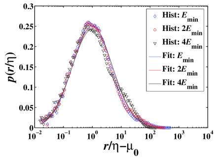
Figure 1: (Color online) Empirical probability density functions of exit distance $r/\eta$ for energy increments $\delta{E}=E_{\min}$, $2E_{\min}$, and $4E_{\min}$. The value of $\mu_{0}$ is the fitted parameter of $\mu$ in the Gaussian distribution.

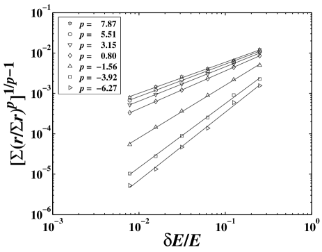
Figure 2: Double logarithmic plots of $[T_{p}(r/\sum{r})]^{1/(p-1)}$ versus $\delta{E}/E$ for different values of $p$. The straight lines are best fits to the data.

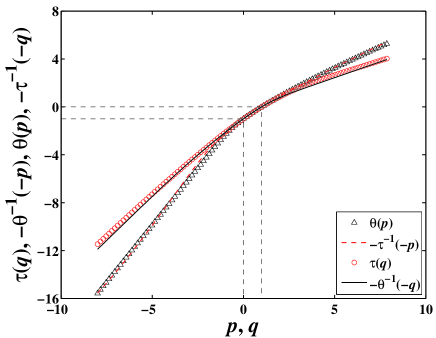
Figure 3: (Color online) Testing the inversion formula of turbulence dissipation energy.