Statistical properties of daily ensemble variables in the Chinese stock markets

Abstract

We study dynamical behavior of the Chinese stock markets by investigating the statistical properties of daily ensemble returns and varieties defined respectively as the mean and the standard deviation of the ensemble daily price returns of a portfolio of stocks traded in China’s stock markets on a given day. The distribution of the daily ensemble returns has an exponential form in the center and power-law tails, while the variety distribution is log-Gaussian in the bulk followed by a power-law tail for large varieties. Based on detrended fluctuation analysis, R/S analysis and modified R/S analysis, we find evidence of long memory in the ensemble returns and strong evidence of long memory in the evolution of variety.

,

1 Introduction

Financial markets are complex systems, in which participants interact with each other and react to external news attempting to gain extra earnings by beating the markets. In the last decades, econophysics has become to flourish since the pioneering work of Mantegna and Stanley in 1995 [1]. Econophysics is an emerging interdisciplinary field, where theories, concepts, and tools borrowed from statistical mechanics, nonlinear sciences, mathematics, and complexity sciences are applied to understand the self-organized complex behaviors of financial markets [2, 3, 4]. Econophysicists have discovered or rediscovered numerous stylized facts of financial markets [2, 5], such as fat tails of return distributions [6, 1, 7, 8, 9, 10, 11, 12, 13], absence of autocorrelations of returns [2], long memory in volatility [14, 15, 16], intermittency and multifractality [7, 17, 18, 19], and leverage effect [20, 21], to list a few.

Recently, Lillo and Mantegna have introduced the conception of ensemble variable treating a portfolio of stocks as a whole [22, 23, 24, 25]. They have defined two quantities, the ensemble return and the variety. The ensemble return ${\mu}$ is the mean of the returns of the portfolio at time $t$, which is a measure of the market direction, while the variety ${\sigma}$ is the standard deviation of all the the returns at time $t$, which characterizes how different the behavior of stocks is. In the time periods when the markets are very volatile, the ensemble returns have larger fluctuations and the varieties are larger as well. It is very interesting to note that there are sharp peaks in the variety time series when the market crashes [24, 25], which is reminiscent of the behavior of volatility. In addition, the daily ensemble return of stocks in the New York Stock Exchange is found to be uncorrelated, while the daily variety has long memory [23]. Despite of such remarkable similarities shared by the ensemble returns and the returns and by the varieties and the volatilities, there are significant difference between these “competing” quantities, especially the shapes of the corresponding distributions.

There are a huge number of studies in the literature showing that emerging stork markets behave differently other than the developed markets in many aspects. In most developed markets, the daily returns have well established fat tails, while the distributions of daily returns are exponential in several emerging markets, e.g., in China [26], Brazil [27], and India [28]. It is very interesting to investigate the statistical properties of the ensemble variables extracted in emerging stock markets, which is the main motivation of the current work. We shall focus on the Chinese stock markets in this paper.

The paper is organized as follows. In Sec. 2, we explain the data set analyzed and define explicitly the ensemble return and variety. Section 3 presents analysis on the probability distributions of the daily ensemble returns and varieties. We discuss in Sec. 4 the temporal correlations of the two quantities, where we adopt R/S analysis and detrended fluctuation analysis (DFA) to estimate the Hurst indexes and perform statistical tests using Lo’s modified R/S statistic. The last section concludes.

2 China’s stock markets

Before the foundation of People’s Republic of China in 1949, the Shanghai Stock Exchange was the third largest worldwide, after the New York Stock Exchange and the London Stock Exchange and its evolution over the period from 1919 to 1949 had enormous influence on other world-class financial markets [29]. After 1949, China implemented policies of a socialist planned economy and the government controlled entirely all investment channels. This proved to be efficient in the early stage of the economy reconstruction, especially for the heavy industry. However, planned economic policies have unavoidably led to inefficient allocation of resources. In 1981, the central government began to issue treasury bonds to raise capital to cover its financial deficit, which reopened the China’s securities markets. After that, local governments and enterprises were permitted to issue bonds. In 1984, 11 state-owned enterprises became share-holding corporations and started to provide public offering of stocks. The establishment of secondary markets for securities occurred in 1986 when over-the-counter markets were set up to trade corporation bonds and shares. The first market for government-approved securities was founded in Shanghai on November 26, 1990 and started operating on December 19 of the same year under the name of the Shanghai Stock Exchange (SHSE). Shortly after, the Shenzhen Stock Exchange (SZSE) was established on December 1, 1990 and started its operations on July 3, 1991. The historical high happened in 2000 when the total market capitalization reached 4,968 billion yuan (55.5% of GDP) with 1,535.4 billion yuan of float market capitalization (17.2% of GDP). The size of the Chinese stock market has increased remarkably.

The data set we used in this paper contains daily records of $n=500$ stocks traded in the SHSE and the SZSE in the period from February 1994 to September 2004. The total number of data points exceeds one million. For each stock price time series, we calculate the daily log-return as follows

$$r_{i}(t)=\ln[P_{i}(t)/P_{i}(t-1)]~{},$$ (1)

where $P_{i}(t)$ is the close price of stock $i$ on day $t$. The ensemble return $\mu(t)$ is then defined by

$$\mu(t)=\frac{1}{n}\sum_{i=1}^{n}r_{i}(t)~{},$$ (2)

while the variety $\sigma(t)$ is defined according to

$$\sigma^{2}(t)=\frac{1}{n}\sum_{i=1}^{n}[r_{i}(t)-\mu(t)]^{2}~{}.$$ (3)

The number of active stocks may vary along time $t$. When a stock $j$ is not traded at time $t$, it is not included in the calculation of $\mu$ and $\sigma$.

Figure 1 illustrates the daily ensemble returns ${\mu}$ and the daily variety ${\sigma}$ in the Chinese stock market as a function of time $t$ from Feb. 1994 to Sep. 2004. An striking feature is observed in both quantities that the amplitude of the envelop decreases along time, which indicates that the Chinese stock markets are becoming less volatile and more efficient.

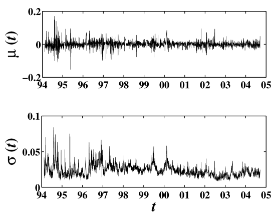
Figure 1: Evolution of the daily ensemble return ${\mu}$ (top) and the daily variety $\sigma$ (bottom) as a function of time.

3 Probability distributions of ensemble variables

The central parts of ensemble returns of NYSE stocks and Nasdaq stocks are exponentially distributed and the negative part decays slower than the positive part [23, 25], while the tails look like outliers in the sense that those ensemble returns are extremely large and can not be modeled by the same exponential distribution as the center part [4]. The Chinese stock markets have the same behavior qualitatively. Figure 2 shows the empirical probability density function of ${\mu}$. We find that the main part of the density function has the following form

$$f(\mu)\sim{\exp}[{-k_{\pm}\mu}]~{},$$ (4)

where $k_{-}=76.1\pm 3.3$ when $-0.06<\mu<0$ and $k_{+}=83.2\pm 3.5$ when $0<\mu<0.06$, which shows that the distribution is asymmetric with the skewness being 0.378. It is interesting to note that the Chinese stock markets have more large ensemble returns than the USA markets, which is consistent with the fact that the Chinese stock markets are extraordinarily volatile.

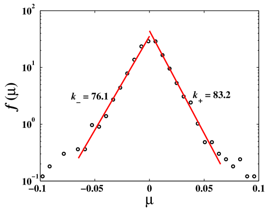
Figure 2: Empirical probability density function of ${\mu}$. The circles represent the real data. The sold lines are the least squares fits to the exponential (4) in the range $[-0.06,0]$ and $[0,0.06]$ and the slopes are $76.1\pm 3.3$ and $83.2\pm 3.5$, respectively.

In order to exploit the tail distribution of the ensemble returns, we adopt the rank-ordering approach [9, 30]. We first sort the $n$ observations in non-increasing order, that is $\mu_{1}\geq\mu_{2}\geq\cdots\geq\mu_{R}\geq\cdots\geq\mu_{n}$, where $R$ is the rank of the observations. Let $C(\mu)=\int_{\mu}^{\infty}f(\mu){\rm{d}}\mu$, then we have

$$nC(\mu_{R})=R$$ (5)

When the probability density of the ensemble variable $\mu$ scales as $f(\mu)\sim\mu^{-({1+\alpha})}$ in the tail, we have [9, 30]

$$\mu_{R}\sim R^{-1/{\alpha}}$$ (6)

for $R\ll N$. A rank-ordering plot of $\ln{\mu_{R}}$ against $\ln{R}$ thus allows us to check if the tails have power law form.

Figure 3 shows the rank-ordering plot of both positive and negative tails, which are approximately power laws. The fitted tail exponents are $\alpha_{-}=3.33\pm 0.06$ for the negative $\mu$ and $\alpha_{+}=2.86\pm 0.07$ for positive $\mu$. This is reminiscent of the inverse cubic law of returns [10, 31, 32].

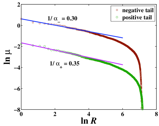
Figure 3: Log-log plot of the rank-ordering $\ln{\mu}$ as a function of $\ln{R}$ for both positive and negative tails(shown in the legend). The plot of the negative tail is translated vertically for clarity. The solid lines are the least squares fit to the data at the interval $0\leq\ln{R}\leq 4$ for the negative tail and $0\leq\ln{R}\leq 3.5$ for the positive tail, and the slopes of the two lines are $0.3\pm 0.005$ and $0.35\pm 0.009$, respectively.

In Fig. 4 is shown the distribution of varieties of the Chinese stock markets. It is evident that the main part of the distribution follows a log-normal form followed by a well established power law tail:

$$f(\sigma)\sim\left\{\begin{array}[]{ll}\exp\left[-\frac{(\ln\sigma-\ln\sigma_{0})^{2}}{2{\rm{Var}}(\sigma)}\right],&{\rm{~{}~{}~{}for~{}not~{}large~{}\sigma}}\\ \sigma^{-\beta},&{\rm{~{}~{}~{}for~{}large~{}\sigma}}\end{array}\right.$$ (7)

where the tail exponent is found to be $\beta=5.3\pm 0.2$. Again, the shape of the variety distribution in the Chinese stock markets is qualitatively the same as in the USA stock markets [23]. Note that the volatilities of most stock markets have log-normal distributions with power-law tails [16]. However, the tail distribution of varieties in China’s stock markets deviates from the inverse cubic law.

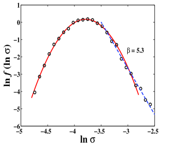
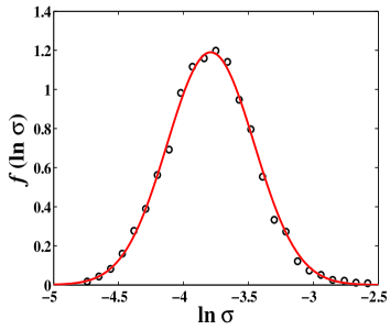
Figure 4: Left: Empirical probability density function of the variety $\sigma$ in double logarithmic coordinates. The continuous line is a parabolic fit while the dashed line shows a power-law distribution of larger varieties ($\ln\sigma>-3.5$). The tail exponent is $\beta=5.3\pm 0.2$. Right: Log-normal distribution of ${\sigma}$.

4 Long memory in the ensemble variables

4.1 Detrended fluctuation analysis

There are a lot of methods developed to extract temporal correlation in time series, among which the detrended fluctuation analysis (DFA) is the most popular method due to its easy implementation and robust estimation even for short time series [33, 34, 35]. DFA was invented originally to study the long-range dependence in coding and noncoding DNA nucleotides sequence [36] and then applied to various fields including finance. In order to investigate the dependence nature of ensemble variables in China’s stock markets, we first adopt the detrended fluctuation analysis.

The DFA is carried out as follows. Consider a time series $x(t)$, $t=1,2,\cdots,N$. We first construct the cumulative sum

$$u(t)=\sum_{i=1}^{t}{x(i)},~{}~{}t=1,2,\cdots,N~{}.$$ (8)

The time interval is then divided into disjoint subintervals of a same length $s$ and fit ${u(t)}$ in each subinterval with a polynomial function, which gives ${u_{s}(t)}$, representing the trend in the subintervals. The detrended fluctuation function $F(s)$ is then calculated

$$F^{2}(s)=\frac{1}{N}\sum_{i=1}^{N}[{u(i)-u_{s}(i)}]^{2}~{}.$$ (9)

Varying $s$, one is able to determine the scaling relation between the detrended fluctuation function ${F(s)}$ and time scale $s$. It is shown that

$$F(s)\sim s^{H}~{},$$ (10)

where $H$ is the Hurst index [33, 37], which is shown to be related to the power spectrum exponent $\eta$ by $\eta=2H-1$ [38, 39] and thus to the autocorrelation exponent $\gamma$ by $\gamma=2-2H$.

Figure 5 plots the detrended fluctuation functions $F(s)$ of the ensemble daily variables ${\mu}$ and ${\sigma}$ as a function of time scale $s$. There are two scaling laws in the curve for ${\mu}$, which are separated at the crossover time lag $\ln{s_{\times}}=3.6$. The Hurst indices for both scaling ranges are $H_{1}=0.66\pm 0.02$ and $H_{2}=0.87\pm 0.02$, respectively. For variety ${\sigma}$, a sound power law scaling relation is observed with a Hurst index $H_{3}=0.93\pm 0.01$. This strong correlation observed here is consistent with that in the USA markets, where the autocorrelation exponent is reported to be $\gamma=0.230\pm 0.006$ [23].

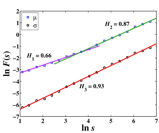
Figure 5: Log-log plot is of the detrended fluctuation functions $F(s)$ of the ensemble daily variables ${\mu}$ and ${\sigma}$ with respect to the time scale $s$. The squares stand for the results calculated from real data of ${\mu}$ and the circles represent the real data of ${\sigma}$. The plot for ${\mu}$ is translated vertically for clarity.

4.2 Rescaled range analysis

To further investigate the correlation structure in the ensemble returns and varieties, we adopt the well-known R/S analysis. R/S analysis was invented by Hurst [40] and then developed by Mandelbrot and Wallis [41, 42], known also as Hurst analysis or rescaled range analysis.

Assume that time series $\{y_{i}:i=1,2,\cdots,s\}$ is a sub-series taken from a longer time series $\{x_{i}:i=1,2,\cdots,N\}$ successively. The cumulative deviation of $\{y_{i}\}$ is defined by

$$X_{s,i}=\sum_{j=1}^{i}\left(y_{j}-\overline{y}\right)~{},$$ (11)

where $\overline{y}$ is the sample average of $\{y_{i}\}$, and the range is given by

$$R_{s}=\max_{1\leq i\leq s}X_{s,i}-\min_{1\leq i\leq s}X_{s,i}$$ (12)

For a time series with long memory, the range rescaled by the sample standard deviation

$$S_{s}=\left[{\frac{1}{n}\sum_{i=1}^{s}{(y_{j}-\overline{y})^{2}}}\right]^{1/2}$$ (13)

scales as a power law with respect to the time scale $s$

$$\frac{R(s)}{S(s)}\sim s^{H}~{},$$ (14)

when $s\to\infty$. There are different algorithms to implement the R/S analysis, based on the partition of sub-series $\{y_{i}\}$. We adopt an algorithm based on random choices of sub-series of size $s$ and averaging over them [43].

The results of the R/S analysis on the daily ensemble returns and varieties are presented in Fig. 6. We observe that both variables exhibit two scaling ranges. For the ensemble returns, the crossover occurs at $\ln{s_{\times}}=4.7$, which should be compared with the crossover at $\ln{s_{\times}}=3.6$ in Fig. 5. The Hurst index for small $s$ is $H_{1}=0.65\pm 0.004$, which is very close to $H_{1}=0.66\pm 0.02$ in Fig. 5. For larger $s$, we have $H_{2}=0.54\pm 0.01$, which is much smaller than $H_{2}=0.87\pm 0.02$ in the detrended fluctuation analysis. This calls for further investigate of possible long memory in the daily ensemble returns. For the daily, varieties, the crossover takes place at $\ln{s_{\times}}=2.8$. The Hurst index for $s\leqslant{s_{\times}}$ is $H_{3}=0.77\pm 0.01$, while for $s\geqslant{s_{\times}}$ we get $H_{4}=0.91\pm 0.003$, which is consistent with $H_{3}=0.93\pm 0.01$ in the detrended fluctuation analysis illustrated in Fig. 5.

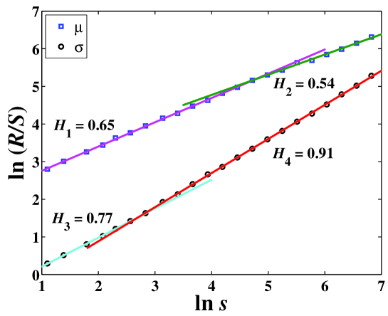
Figure 6: R/S analysis of the daily ensemble returns and the daily varieties. The squares stand for the results calculated from real data of ${\mu}$ and the circles represent the real data of ${\sigma}$. The two lines are the least squares fit to their results respectively. The plot for ${\mu}$ is translated vertically for clarity.

4.3 Statistical tests of long memory

The information extracted from the DFA and the R/S analysis performed on the variety is consistent, where both methods give a large value of Hurst index. However, the situation is quite different when the ensemble is concerned. The Hurst indexes for large time scale $s$ obtained from the two methods are both not far away from $H=0.5$. Due to the subtlety of the issue of long memory, we provide further statistical tests for both ensemble variables, adopting Lo’s modified R/S statistic [44].

Consider a stationary time series of size $n$. The modified R/S statistic is given by [44]

$$Q_{n}=R_{n}/\hat{S}_{n}(q)~{},$$ (15)

where $R_{n}$ is the range of cumulative deviations defined in Eq. (12) and $\hat{S}_{n}(q)$ is defined by

$$\hat{S}_{n}^{2}(q)=S_{n}^{2}+2\sum_{j=1}^{q}\omega_{j}(q)\rho_{j}=S_{n}^{2}+2\sum_{j=1}^{q}\left(1-\frac{j}{q-1}\right)\rho_{j}~{},$$ (16)

where $S_{n}$ is the standard deviation defined in Eq. (13) and $\rho_{j}=\frac{1}{n}\sum_{i=j+1}^{n}(y_{i}-\overline{y})(y_{i-j}-\overline{y})$ is the autocovariance of the time series. If the time series has short-term memory, the statistic variable

$$V_{n}(q)=\frac{1}{\sqrt{n}}Q_{n}(q)$$ (17)

has a finite positive value whose cumulative distribution reads

$$P(V)=1+2\sum_{k=1}^{\infty}(1-4k^{2}V^{2}){\rm{e}}^{k^{2}V^{2}}~{}.$$ (18)

The fractiles can be estimated from Eq. (18): for a bilateral test of 5% significance, we have $V_{0.025}=0.809$ and $V_{0.975}=1.862$. When the time series has long-term memory, it is proved that $R_{n}$ trends to the Brownian bridge variable $V_{H}$, while the variable $S_{n}^{2}/(n\hat{S}_{n}(q))$ tends to $0$ or $\infty$ for large $q$, that is

$$V_{n}(q)=\frac{1}{\sqrt{n}}Q_{n}(q)=\left\{\begin{array}[]{ll}0,&~{}~{}~{}~{}~{}H\in(0,0.5)\\ \infty,&~{}~{}~{}~{}~{}H\in(0.5,1)\end{array}\right.$$ (19)

These properties allow us to distinguish short memory from long memory. The null hypothesis and its alternative hypothesis may be expressed by

$H_{0}$: The time series under consideration has short memory;
$H_{1}$: The time series under consideration has long memory.

The test is performed at the $\alpha$ significant level to accept or reject the null hypothesis according to whether $V_{n}(q)$ is contained in the interval $[V_{\alpha},V_{1-\alpha}]$ or not, where $F(V_{\alpha})=\alpha/2$ and $F(V_{1-\alpha})=1-\alpha/2$. When $V_{n}(q)\notin[V_{\alpha},V_{1-\alpha}]$, the null hypothesis $H_{0}$ can be rejected such that the time series has long memory.

We have used $q=36$, $72$, $108$, and $144$ in the tests. The tests are performed on the whole time series from 1994/02/14 to 2004/09/15 and its subintervals. The results for ${\mu}$ are presented in Table 1. For the whole time series, the hypothesis that there is no long memory can not be rejected. However, the alternative long memory in several subintervals is significant at the $\alpha=5\%$ level. It is thus possible there exists long memory in ${\mu}$ in the Chinese stock markets intermittently, which is not unreasonable due to the inefficiency of the emerging markets.

Table 1: Statistical test of long memory in the daily ensemble return ${\mu}$ using the modified R/S statistic $V_{n}(q)=Q_{n}(q)/{\sqrt{n}}$, which is compared with the classical R/S statistic $\widetilde{V}_{n}=\widetilde{Q}_{n}/\sqrt{n}$, where $\widetilde{Q}_{n}=R/S$.

Time Period	$n$	$\widetilde{V}_{n}$	$V_{n}(36)$	$V_{n}(72)$	$V_{n}(108)$	$V_{n}(144)$
1994/02/14 - 2004/09/15	2568	1.81	1.66	1.70	1.70	1.72
1994/02/14 - 1999/05/18	1284	$2.11^{\star}$	$2.03^{\star}$	$2.17^{\star}$	$2.19^{\star}$	$2.16^{\star}$
1999/05/19 - 2004/09/15	1284	$1.93^{\star}$	1.55	1.47	1.46	1.50
1994/02/14 - 1996/09/19	642	$2.38^{\star}$	$2.35^{\star}$	$2.55^{\star}$	$2.66^{\star}$	$2.88^{\star}$
1996/09/20 - 1999/05/18	642	$2.00^{\star}$	$1.88^{\star}$	$2.00^{\star}$	$2.09^{\star}$	$1.96^{\star}$
1999/05/19 - 2002/01/14	642	$2.45^{\star}$	1.85	1.73	1.71	1.73
2002/01/15 - 2004/09/15	642	$2.89^{\star}$	$2.81^{\star}$	$2.77^{\star}$	$3.01^{\star}$	$3.47^{\star}$

Table 2 presents the tests for the daily varieties ${\sigma}$. The long memory hypothesis is significant at the $\alpha=5\%$ level for all values of $q$ in all subintervals investigated. For the whole time series, the null hypothesis $H_{0}$ is rejected for $q=36$ and $q=72$. For larger values of $q$, the tests show that there is no significant long memory. Since the definition of the statistic $V_{q}(n)$ amounts to remove “autocorrelation” up to $q$ trading days, the modified R/S test is biased to over-reject long memory [45]. Therefore, we argue that the daily varieties ${\sigma}$ are long-term correlated.

Table 2: Statistical test of long memory in the daily ensemble return using ${\sigma}$ the modified R/S statistic $V_{n}(q)$, which is compared with the classical R/S statistic $\widetilde{V}_{n}$.

Time Period	$n$	$\widetilde{V}_{n}$	$V_{n}(36)$	$V_{n}(72)$	$V_{n}(108)$	$V_{n}(144)$
1994/02/14 - 2004/09/15	2568	$11.18^{\star}$	$2.67^{\star}$	$2.07^{\star}$	1.81	1.64
1994/02/14 - 1999/05/18	1284	$19.17^{\star}$	$5.43^{\star}$	$4.50^{\star}$	$4.12^{\star}$	$3.85^{\star}$
1999/05/19 - 2004/09/15	1284	$20.11^{\star}$	$4.43^{\star}$	$3.48^{\star}$	$3.08^{\star}$	$2.84^{\star}$
1994/02/14 - 1996/09/19	642	$19.61^{\star}$	$5.70^{\star}$	$4.82^{\star}$	$4.59^{\star}$	$4.49^{\star}$
1996/09/20 - 1999/05/18	642	$30.15^{\star}$	$8.77^{\star}$	$7.66^{\star}$	$7.27^{\star}$	$6.94^{\star}$
1999/05/19 - 2002/01/14	642	$27.09^{\star}$	$6.09^{\star}$	$4.99^{\star}$	$4.67^{\star}$	$4.49^{\star}$
2002/01/15 - 2004/09/15	642	$42.99^{\star}$	$11.52^{\star}$	$9.49^{\star}$	$8.61^{\star}$	$8.14^{\star}$

5 Conclusion

The ensemble variables ${\mu}$ and ${\sigma}$ are important for studying the behavior of financial markets as a whole complex system, instead of individual stocks. In this paper, we have studied the statistical properties of the daily ensemble returns and daily varieties of 500 stocks traded in the Shanghai Stock Exchanges and the Shenzhen Stock Exchanges from 1994/02/14 to 2004/09/15.

The daily ensemble returns ${\mu}$ are found to have exponential distributions followed by power-law tails. The negative ensemble returns decay more slowly than the positive part. The negative and positive tail exponents are $\alpha_{-}=3.33\pm 0.06$ and $\alpha_{+}=2.86\pm 0.07$. On the other hand, the daily varieties ${\sigma}$ exhibit a log-normal distribution for not large values and a power-law form on the tail for large values. The tail exponent is estimated to be $\beta=5.3\pm 0.2$.

There are numerous controversies on the efficiency of the Chinese stock markets, with slight bias to inefficiency [29]. Using detrended fluctuation analysis, R/S analysis and modified R/S analysis, we have shown that the daily ensemble returns have long-term memory in several time periods, which is nevertheless insignificant in the whole time series. Specifically, the long memory disappears only in the time period from 1999/05/19 to 2002/01/14. This indicates that the Chinese stock markets do not follow random walks in most time periods. The long-term memory in the daily varieties is quite strong with a large hurst index $H=0.91\sim 0.93$.

Acknowledgments:

This work was supported by the Natural Science Foundation of China through Grant 70501011.

References

- [1] R. N. Mantegna, H. E. Stanley, Scaling behaviour in the dynamics of an economic index, Nature 376 (1995) 46–49.
- [2] R. N. Mantegna, H. E. Stanley, An Introduction to Econophysics: Correlations and Complexity in Finance, Cambridge University Press, Cambridge, 2000.
- [3] J.-P. Bouchaud, M. Potters, Theory of Financial Risks: From Statistical Physics to Risk Management, Cambridge University Press, Cambridge, 2000.
- [4] D. Sornette, Why Stock Markets Crash: Critical Events in Complex Financial Systems, Princeton University Press, Princeton, 2003.
- [5] R. Cont, Empirical properties of asset returns: Stylized facts and statistical issues, Quant. Finance 1 (2001) 223–236.
- [6] B. Mandelbrot, The variation of certain speculative prices, J. Business 36 (1963) 394–419.
- [7] S. Ghashghaie, W. Breymann, J. Peinke, P. Talkner, Y. Dodge, Turbulent cascades in foreign exchange markets, Nature 381 (1996) 767–770.
- [8] A. Johansen, D. Sornette, Stock market crashes are outliers, Eur. Phys. J. B 1 (1998) 141–143.
- [9] J. Laherrere, D. Sornette, Stretched exponential distributions in nature and economy: “Fat tails” with characteristic scales, Eur. Phys. J. B 2 (1998) 525–539.
- [10] P. Gopikrishnan, M. Meyer, L. A. N. Amaral, H. E. Stanley, Inverse cubic law for the distribution of stock price variations, Eur. Phys. J. B 3 (1998) 139–140.
- [11] P. Gopikrishnan, V. Plerou, L. Amaral, M. Meyer, H. Stanley, Scaling of the distribution of fluctuations of financial market indices, Phys. Rev. E 60 (1999) 5305–5316.
- [12] V. Plerou, P. Gopikrishnan, L. A. N. Amaral, M. Meyer, H. E. Stanley, Scaling of the distribution of price fluctuations of individual companies, Phys. Rev. E 60 (1999) 6519–6529.
- [13] Y. Malevergne, V. Pisarenko, D. Sornette, Empirical distributions of stock returns: Between the stretched exponential and the power law?, Quant. Finance 5 (2005) 379–401.
- [14] Y.-H. Liu, P. Cizeau, M. Meyer, C. Peng, H. E. Stanley, Correlations in economic time series, Physica A 245 (1997) 437–440.
- [15] A. Arnéodo, J.-F. Muzy, D. Sornette, “Direct” causal cascade in the stock market, Eur. Phys. J. B 2 (1998) 277–282.
- [16] Y.-H. Liu, P. Gopikrishnan, P. Cizeau, M. Meyer, C.-K. Peng, H. E. Stanley, Statistical properties of the volatility of price fluctuations, Phys. Rev. E 60 (1999) 1390–1400.
- [17] R. N. Mantegna, H. E. Stanley, Turbulence and financial markets, Nature 383 (1996) 587–588.
- [18] K. Ivanova, M. Ausloos, Low -moment multifractal analysis of Gold price, Dow Jones Industrial Average and BGL-USD exchange rate, Eur. Phys. J. B 8 (1999) 665–669.
- [19] B. B. Mandelbrot, Scaling in financial prices, II: Multifractals and the star equation, Quant. Finance 1 (2001) 124–130.
- [20] J.-P. Bouchaud, A. Matacz, M. Potters, Leverage effect in financial markets: The retarded volatility model, Phys. Rev. Lett. 87 (2001) 228701.
- [21] J.-P. Bouchaud, M. Potters, More stylized facts of financial markets: Leverage effect and downside correlations, Physica A 299 (2001) 60–70.
- [22] F. Lillo, R. N. Mantegna, Symmetry alteration of ensemble return distribution in crash and rally days of financial markets, Eur. Phys. J. B 15 (2000) 603–606.
- [23] F. Lillo, R. N. Mantegna, Valiety and volatility in financial markets, Phys. Rev. E 62 (2000) 6126–6134.
- [24] F. Lillo, R. N. Mantegna, Empirical properties of the variety of a financial portfolio and the single-index model, Eur. Phys. J. B 20 (2001) 503–509.
- [25] F. Lillo, R. N. Mantegna, Ensemble properties of securities traded in the NASDAQ market, Physica A 299 (2001) 161–167.
- [26] S.-J. Wang, C.-S. Zhang, Microscopic model of financial markets based on belief propagation, Physica A 354 (2005) 496–504.
- [27] L. C. Miranda, R. Riera, Truncated Lévy walks and an emerging market economic index, Physica A 297 (2001) 509–520.
- [28] K. Matia, M. Pal, H. Salunkay, H. E. Stanley, Scale-dependent price fluctuations for the Indian stock market, Europhys. Lett. 66 (2004) 909–914.
- [29] D.-W. Su, Chinese Stock Markets: A Research Handbook, World Scientific, Singapore, 2003.
- [30] D. Sornette, L. Knopoff, Y. Y. Kagan, C. Vanneste, Rank-ordering statistics of extreme events: Application to the distribution of large earthquakes, J. Geophys. Res. 101 (1996) 13883–13893.
- [31] X. Gabaix, P. Gopikrishnan, V. Plerou, H. E. Stanley, Understanding the cubic and half-cubic laws of financial fluctuations, Physica A 324 (2003) 1–5.
- [32] X. Gabaix, P. Gopikrishnan, V. Plerou, H. E. Stanley, A theory of power-law distributions in financial market fluctuations, Nature 423 (2003) 267–270.
- [33] M. Taqqu, V. Teverovsky, W. Willinger, Estimators for long-range dependence: An empirical study, Fractals 3 (1995) 785–798.
- [34] A. Montanari, M. S. Taqqu, V. Teverovsky, Estimating long-range dependence in the presence of periodicity: An empirical study, Mathematical and Computer Modelling 29 (10-12) (1999) 217–228.
- [35] B. Audit, E. Bacry, J.-F. Muzy, A. Arnéodo, Wavelet-based estimators of scaling behavior, IEEE Transactions on Information Theory 48 (2002) 2938–2954.
- [36] C.-K. Peng, S. V. Buldyrev, S. Havlin, M. Simons, H. E. Stanley, A. L. Goldberger, Mosaic organization of DNA nucleotides, Phys. Rev. E 49 (1994) 1685–1689.
- [37] J. W. Kantelhardt, E. Koscielny-Bunde, H. H. A. Rego, S. Havlin, A. Bunde, Detecting long-range correlations with detrended fluctuation analysis, Physica A 316 (2001) 441–454.
- [38] P. Talkner, R. Weber, Power spectrum and detrended fluctuation analysis: Application to daily temperatures, Phys. Rev. E 62 (2000) 150–160.
- [39] C. Heneghan, G. McDarby, Establishing the relation between detrended fluctuation analysis and power spectral density analysis for stochastic processes, Phys. Rev. E 62 (2000) 6103–6110.
- [40] H. E. Hurst, Long-term storage capacity of reservoirs, Transactions of American Society of Civil Engineers 116 (1951) 770 808.
- [41] B. Mandelbrot, J. Wallis, Computer experiments with fractional Gaussian noise. Part 2, rescaled ranges and spectra, Water Resource Research 5 (1969) 242–259.
- [42] B. Mandelbrot, J. Wallis, Robustness of the rescaled range R/S in the measurement of noncyclic long run statistical dependence, Water Resource Research 5 (1969) 967–988.
- [43] W.-X. Zhou, H.-F. Liu, X. Gong, F.-C. Wang, Z.-H. Yu, Long-term temporal dependence of droplets transiting through a fixed spatial point in gas-liquid two-phase turbulent jets, preprint (2005).
- [44] A. W. Lo, Long-term memory in stock market prices, Econometrica 59 (1991) 1279–1313.
- [45] V. Teverovsky, M. Taqqu, W. Willinger, A critical look at Lo’s modified R/S statistic, J. Stat. Plann. Inference 80 (1999) 211–227.