Analysis of Non-stationary Data for Heart-Rate Fluctuations in Terms of Drift and Diffusion Coefficients

Abstract

We describe a method for analyzing the stochasticity in the non-stationary data for the beat-to-beat fluctuations in the heart rates of healthy subjects, as well as those with congestive heart failure. The method analyzes the returns time series of the data as a Markov process, and computes the Markov time scale, i.e., the time scale over which the data are a Markov process. We also construct an effective stochastic continuum equation for the return series. We show that the drift and diffusion coefficients, as well as the amplitude of the returns time series for healthy subjects are distinct from those with CHF. Thus, the method may potentially provide a diagnostic tool for distinguishing healthy subjects from those with congestive heart failure, as it can distinguish small differences between the data for the two classes of subjects in terms of well-defined and physically-motivated quantities.

PACS: 05.10.Gg, 05.40.-a,05.45.Tp, 87.19.Hh

]

Introduction

Cardiac interbeat intervals fluctuate in a complex manner [1, 2, 3, 4, 5, 6, 7]. Recent studies reveal that under normal conditions, beat-to-beat fluctuations in the heart rate may display extended correlations of the type typically exhibited by dynamical systems far from equilibrium. It has been shown [2], for example, that the various stages of sleep may be characterized by long-range correlations in the heart rates, separated by a large number of beats.

The analysis of the interbeat fluctuations in the heart rates belong to a much broader class of many natural, as well as man-made, phenomena that are characterized by a degree of stochasticity. Turbulent flows, fluctuations in the stock market prices, seismic recordings, the internet traffic, pressure fluctuations in chemical reactors, and the surface roughness of many materials and rock [8], are but a few examples of such phenomena and systems. A long standing problem has been the development of an effective reconstruction method for such phenomena. That is, given a set of data for certain characteristics of such phenomena (for example, the interbeat fluctuations in the heart rates), one would like to develop an effective equation that can reproduce the data with an accuracy comparable to the measured data. Although many methods have been suggested in the past, and considerable progress has been made, the problem remains, to a large extent, unsolved.

In many cases the stochastic process to be analyzed is non-stationary. If the process also exhibits extended correlations, then deducing its statistical properties by the standard methods of analyzing such processes is very difficult. One approach to analyze such processes was proposed by Stanley and co-workers [1, 3, 5, 20, 21, 22, 23, 24] and others [25, 26, 27, 28, 29]. They studied data for heart-rate fluctuations, for both healthy subjects and those with congestive heart failure (CHF), in terms of self-affine fractal distributions, such as the fractional Brownian motion (FBM). The FBM is a non-stationary stochastic process which induces long-range correlations, the successive increments of which are, however, stationary and follow a Gaussian distribution. The power spectrum of a FBM is given by, $S(f)\propto f^{-(2H+1)}$, where $H$ is the Hurst exponent that characterizes the type of the correlations that the data contain. Thus, one may distinguish healthy subjects from those with CHF in terms of the numerical value of $H$ associated with the data: negative or antipersistent correlations for $H<1/2$, as opposed to positive or persistent correlations for $H>1/2$. The analysis of Stanley and co-workers indicated that there may indeed be long-range correlations in heart-rate fluctuations data that can be characterized by the FBM and similar fractal distributions. In addition, the data for healthy subjects seem to be characterized by $H<1/2$, whereas those with CHF by $H>1/2$. This was a significant discovery over the traditional methods of analyzing non-stationary data for heart-rate fluctuations.

However, values of the Hurst exponent $H$ associated with the two groups of subjects are non-universal. Thus, it would, for example, be difficult to distinguish the two groups of subjects if their associated Hurst exponents are both close to 1/2. In addition, the FBM is a non-self-averaging distribution, i.e., given a fixed Hurst exponent $H$, each realization of a FBM may be significantly different from its other realizations with the same $H$. As a result, estimating $H$ alone and characterizing the data by a FBM cannot enable one to predict the future trends of the data. One may also analyze such data by the deterended fluctuating analysis [2, 3, 4, 5] which, in many cases, is capable of yielding accurate and insightful information about the nature of the data.

Recently, a novel method of analyzing stochastic processes was introduced [9, 10, 11, 12]. It was shown that by analyzing stochastic phenomena as Markov processes and computing their Markov time (or length) scale (that is, the time scale over which the process can be thought of as Markov), one may reconstruct the original process with similar statistical properties by constructing an effective equation that governs the process. The constructed equation helps one to understand the nature and properties of the stochastic process. The method utilizes a set of experimental data for a phenomenon which contains a degree of stochasticity, and constructs a simple equation that governs the phenomenon [9, 10, 11, 12, 13, 14, 15, 16]. The method is quite general; it is capable of providing a rational explanation for complex features of the phenomenon. More significantly, it requires no scaling feature.

In this paper we describe a method for analyzing non-stationary data, and then utilize it to study the interbeat fluctuations in the heart rates. We show that the application of the method to the analysis of interbeat fluctuations in the heart rates may potentially lead to a novel method for distinguishing healthy subjects from those with CHF.

The plan of this paper is as follows. In the next section, we describe the method. We then utilize the method to analyze data for heart-rate fluctuations in human subjects.

Markov Analysis of Non-Stationary Data

Given a (discrete) non-stationary time series $r_{i}$, we introduce a quantity $x_{i}$, called the return of $r_{i}$, defined by

$$x_{i}=\ln(r_{i+1}/r_{i})\;,$$ (1)

where $r_{i}$ is the value of the stochastic quantity at step $i$. If there are long-range positive correlations in the series, then $r_{i}$ and $r_{i+1}$ are close in values and, therefore, we expect the series $x_{i}$ to have very small values for all $t$. For white noise, as well as data that exhibit negative or anti-correlations, $r_{i}$ and $r_{i+1}$ can be completely different and, therefore, the time series $x_{i}$ will fluctuate strongly.

Figures 1 and 2 present the typical data $r_{i}$ and the corresponding returns $x_{i}$ for healthy subjects and those with CHF. The number of data is of the order of 30,000-40,000, taken over a period of about 6 hours. It is evident that the returns series for the subjects with CHF has small amplitudes, implying that the $r_{i}$ data set has long-range positive correlations, which is consistent with the previous analysis [1]. It can be verified straightforwardly that the series $x_{i}$ is stationary, by measuring the stability of its average and variance in a moving window (that is, over a period of time which varies over the length of the series).

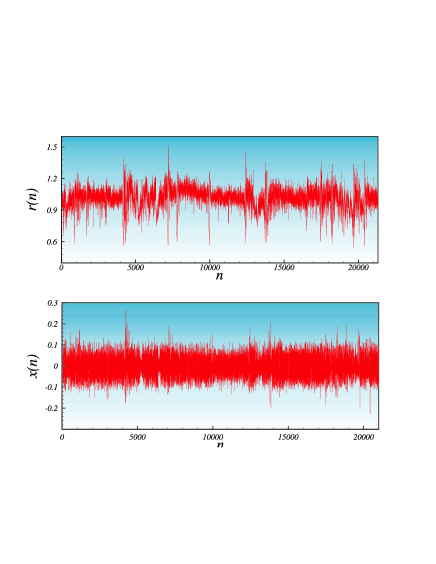
FIG. 1.: Interbeats fluctuations of healthy subjects (top), and its returns (bottom).

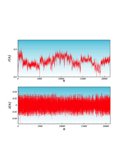
FIG. 2.: Interbeats fluctuations of subjects with congestive heart failure (top), and its returns (bottom).

Due to the stationarity of the series $x(t)$, we can construct an effective stochastic equation for the returns series of the two groups of subjects, and distinguish the data for healthy subjects from those with CHF. The procedure to do so involves two key steps:

(1) Computing the Markov time scale (MTS) $t_{M}$ constitutes the first step. $t_{M}$ is the minimum time interval over which the data can be considered as a Markov process [9, 10, 11, 12, 17]. As is well-known, a given stochastic process with a degree of randomness may have a finite or even an infinite $t_{M}$. To estimate the MTS $t_{M}$, we note that a complete characterization of the statistical properties of stochastic fluctuations of a quantity $x(t)$ in terms of a parameter $t$ requires the evaluation of the joint probability distribution function (PDF) $P_{n}(x_{1},t_{1};\cdots;x_{n},t_{n})$ for an arbitrary $n$, the number of the data points. If a stochastic phenomenon is a Markov process, an important simplification can be made as $P_{n}$, the $n$-point joint PDF, is generated by the product of the conditional probabilities, $p(x_{i+1},t_{i+1}|x_{i},t_{i})$, for $i=1,\cdots,n-1$.

The simplest way to determine $t_{M}$ for stationary data is by using the least-square test. The rigorous mathematical definition of a Markov process is given [18] by

$$P(x_{k},t_{k}|x_{k-1},t_{k-1};\cdots;x_{1},t_{1};x_{0},t_{0})$$ (2)

(3)

$$=P(x_{k},t_{k}|x_{k-1},t_{k-1})\;.$$ (4)

Intuitively, the physical interpretation of a Markov process is that it ”forgets its past.” In other words, only the closest ”event” to $x_{k}$, say $x_{k-1}$ at time $t_{k-1}$, is relevant to the probability of the event $x_{k}$ at $t_{k}$. Hence, the ability for predicting the event $x_{k}$ is not enhanced by knowing its values in steps prior to the the most recent one. Therefore, an important simplification that is made for a Markov process is that, the conditional multivariate joint PDF is written in terms of the products of simple two parameter conditional PDF’s [18] as (5)

$$P(x_{k},t_{k};x_{k-1},t_{k-1};\cdots;x_{1},t_{1}|x_{0},t_{0})$$ (5)

(6)

$$=\prod_{i=1}^{k}P(x_{i},t_{i}|x_{i-1},t_{i-1})\;.$$ (7)

Testing Eq. (5) for large values of $k$ is beyond the current computational capability. For $k=3$ (three points or events), however, the working equation, given by,

$$P(x_{3},t_{3}|x_{2},t_{2};x_{1},t_{1})=P(x_{3},t_{3}|x_{2},t_{2})\;,$$ (8)

should hold for any value of $t_{2}$ in the interval $t_{1}<t_{2}<t_{3}$. A process is then Markovian if Eq. (8) is satisfied for a certain time separation $t_{3}-t_{2}$, in which case, $t_{M}=t_{3}-t_{2}$. Thus, to compute the $t_{M}$ we use a fundamental theory of probability according to which we write any three-point PDF in terms of the conditional probability functions as,

$$P(x_{3},t_{3};x_{2},t_{2};x_{1},t_{1})$$ (9)

(10)

$$=P(x_{3},t_{3}|x_{2},t_{2};x_{1},t_{1})P(x_{2},t_{2};x_{1},t_{1}).$$ (11)

Using the properties of Markov processes to substitute Eq. (9), we obtain,

$$P_{\rm Markov}(x_{3},t_{3};x_{2},t_{2};x_{1},t_{1})$$ (12)

(13)

$$=P(x_{3},t_{3}|x_{2},t_{2})P(x_{2},t_{2};x_{1},t_{1}).$$ (14)

We then compare the deviation of $P_{\rm Markov}$ from that given by Eq. (9). Using the least square method [10], we write:

$$\chi^{2}=\int dx_{3}dx_{2}dx_{1}\times$$ (15)

(16)

$$\frac{[P(x_{3},t_{3};x_{2},t_{2};x_{1},t_{1})-P_{\rm Markov}(x_{3},t_{3};x_{2},t_{2};x_{1},t_{1})]^{2}}{\sigma^{2}+\sigma_{\rm Markov}^{2}}\;,$$ (17)

where $\sigma^{2}$ and $\sigma^{2}_{\rm Markov}$ are the corresponding variances of terms in the nominator. Thus, one should plot the reduced chi-square, $\chi^{2}_{\nu}=\chi^{2}/{\cal N}$ (with ${\cal N}$ being the number of degrees of freedom), as a function of the time scale $t_{3}-t_{2}$. Then, $t_{M}=t_{3}-t_{2}$ for that value of $t_{3}-t_{2}$ for which $\chi^{2}_{\nu}$ either achieves a minimum or becomes flat and does not change anymore; see Figure 3.

On the other hand, a necessary condition for a stochastic phenomenon to be a Markov process is that the Chapman-Kolmogorov (CK) equation (18),

$$P(x_{3},t_{3}|x_{1},t_{1})=\int\hbox{d}x_{2}\;P(x_{3},t_{3}|x_{2},t_{2})\;P(x_{2},t_{2}|x_{1},t_{1})\;,$$ (18)

should hold for the time separation $t_{3}-t_{2}$, in which case, $t_{M}=t_{3}-t_{2}$. Therefore, to test whether the time series $x(t)$ is a Matkov process, one should check the validity of the CK equation for describing the process using different $x_{1}$ by comparing the directly-evaluated conditional probability distributions $P(x_{3},t_{3}|x_{1},t_{1})$ with the one calculated according to right side of Eq. (18).

(2) Estimation of the Kramers-Moyal coefficients is the second step of constructing an effective equation for describing the series $x_{i}$. The CK equation is an evolution equation for the distribution function $P(x,t)$ at any time $t$. When formulated in differential form, the CK equation yields the Kramers-Moyal (KM) expansion [18], given by,

$$\frac{\partial}{\partial t}P(x,t)=\sum_{n=1}^{\infty}(-\frac{\partial}{\partial x})^{n}[D^{(n)}(x)P(x,t)]\;.$$ (19)

The coefficients $D^{(n)}(x,t)$ are called the KM coefficients. They are estimated directly from the data, the conditional probability distributions, and the moments $M^{(n)}$ defined by,

$$M^{(n)}=\frac{1}{\Delta t}\int dx^{\prime}(x^{\prime}-x)^{n}P(x^{\prime},t+\Delta t|x,t),$$ (20)

(21)

$$D^{(n)}(x,t)=\frac{1}{n!}\hskip 5.69046pt\lim_{\Delta t\to 0}M^{(n)}.$$ (22)

According to the Pawula’s theorem, for a process with $D^{(4)}\sim 0$ all the $D^{(n)}$ with $n\geq 3$ vanish, in which case the KM expansion reduces to the Fokker-Planck equation, also known as the Kolomogrov equation [18]:

$$\frac{\partial}{\partial t}P(x,t)=\left[-\frac{\partial}{\partial x}D^{(1)}(x,t)+\frac{\partial^{2}}{\partial x^{2}}D^{(2)}(x,t)\right]P(x,t)\;.$$ (23)

Here $D^{(1)}(x,t)$ is the drift coefficient, representing the deterministic part of the process, and $D^{(2)}(x,t)$ is the diffusion coefficient that represents the stochastic part.

We now apply the above method to the fluctuations in the human heartbeats of both healthy subjects and those with CHF. As mentioned in the Introduction, several studies [5, 6, 10, 11, 12, 19, 20, 21] indicate that, under normal conditions, the beat-to-beat fluctuations in the heart rate may display extended correlations of the type typically exhibited by dynamical systems far from equilibrium, and that the two groups of subjects may be distinguished from one another by a Hurst exponent. We show that the drift and diffusion coefficients (as defined above) of the interbeat fluctuations of healthy subjects and patients with CHF have distinct behavior, when analyzed by the method we propose in this paper, hence enabling one to distinguish the two groups of the subjects.

We analyzed both daytime (12:00 pm to 18:00 pm) and nighttime (12:00 am to 6:00 am) heartbeat time series of healthy subjects, and the daytime records of patients with CHF. Our data base includes 10 healthy subjects (7 females and 3 males with ages between 20 and 50, and an average age of 34.3 years), and 12 subjects with CHF (3 females and 9 males with ages between 22 and 71, and an average age of 60.8 years). Figures 1 and 2 present the data.

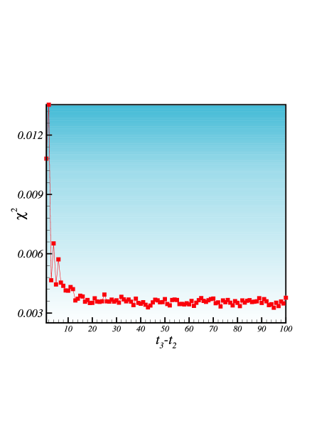
FIG. 3.: $\chi^{2}_{\nu}$ values for a typical subject with CHF for several time scales.

We first estimate the Markov time scale $t_{M}$ for the returns series of the interbeat fluctuations, using the chi-square method described above. In Figure 3 the results for the $\chi^{2}_{\nu}$ values for a subject with CHF are shown. For the healthy subjects we find the average $t_{M}$ for the returns, for both the day- and nighttime data, to be (all the values are measured in units of the average time scale for the beat-to-beat times of each subject), $t_{M}=10$. On the other hand, for the daytime records of the patients with CHF, the estimated average $t_{M}$ is, $t_{M}=20$. Therefore, the data for the healthy subjects are characterized by $t_{M}$ values that are smaller than that of the patients with CHF by a significant factor of 2.

We then check the validity of the CK equation for several $x_{1}$ triplets by comparing the directly-evaluated conditional probability distributions $P(x_{3},t_{3}|x_{1},t_{1})$ with the ones calculated according to right side of Eq. (18). Here, $x$ represents the returns. In Figure 4, the two differently-computed PDFs are compared. Assuming the statistical errors to be the square root of the number of events in each bin, we find that the two PDFs are statistically identical.

FIG. 4.: Test of Chapman-Kolmogorov equation for the time separation between $t_{3}$ and $t_{1}$ equal to the Markov time scale, for $x_{1}=-6\times 10^{-2}$, $x_{1}=0$, and $x_{1}=6\times 10^{-2}$. Squares and triangles represent, respectively, the directly-evaluated PDF and that computed according to the right side of Eq. (18). For clarity, the PDFs are shifted in the vertical directions.

Using Eq. (20) directly we calculate the drift and diffusion coefficients, $D^{(1)}(x)$ and $D^{(2)}(x)$, for the entire set of data for the healthy subjects, as well as those with CHF. The corresponding $D^{(1)}(x)$ and $D^{(2)}(x)$ are displayed in Figure 5. We find that, these coefficients provide another important indicator for distinguishing the ill from the healthy subjects: The drift $D^{(1)}$ and the diffusion coefficients $D^{(2)}(x)$ follow, respectively, linear and quadratic equations in $x$ with distinct coefficients for the healthy subjects and patients with CHF. The analysis of the data yields the following estimate for the healthy subjects (averaged over the samples),

$$D^{(1)}(x)=-0.1x\;,$$ (26)

$$D^{(2)}(x)=3.7\times 10^{-5}-6.6\times 10^{-5}x+0.06x^{2}\;,$$

with $-0.15<x<0.15$, whereas for the patients with CHF we find that,

$$D^{(1)}(x) = -0.06x\;,$$ (27)

$$D^{(2)}(x) = 8.6\times 10^{-6}-2.7\times 10^{-5}x+0.03x^{2}\;.$$ (29)

with $-0.04<x<0.04$.

We find two important differences between the heartbeat dynamics of the two classes of subjects:

(1) Compared with the healthy subjects, the drift and diffusion coefficients for the patients with CHF are small.

(2) The fluctuations of the returns for healthy subjects are distinct from those with CHF. They also fluctuate over different intervals, indicating that the returns data for the healthy subjects fluctuate over large interval. The fluctuations intervals are, $-0.04<x<0.04$ and $-0.15<x<0.15$ for patients with CHF and healthy subjects, respectively. Hence, we suggest that one may use the drift and diffusion coefficients magnitudes, as well as the fluctuations intervals for the returns, for characterizing the dynamics of human heartbeats, and to distinguish healthy subjects from those with CHF.

I Discussions

Lin [30] argued that the daytime heart rate variability of healthy subjects may exhibit discrete scale-invariance (DSI). A stochastic process $x(t)$ possesses continuous scale-invariant symmetry if its distribution is preserved under a change of variables, $t\to\lambda t$ and $x\to x/\mu$, where $\lambda$ and $\mu$ are real numbers, so that,

$$x(t)=\frac{1}{\mu}x(\lambda t)\;.$$ (30)

If Eq.(30) holds only for a countable (discrete) set of values of $\lambda$, $x(t)$ is said to possess DSI, which implies a power-law behavior for $x(t)$ that has a log-periodic correction of frequency $1/\log\lambda$, so that

$$x(t)=t^{\gamma}F(\log t/\log\lambda)\;,$$ (31)

with, $\gamma=\log\mu/\log\lambda$, with $F(x)=F(x+1)$ being a period scaling function. Generally speaking, one may write, $x(t)=c(t)t^{\zeta}$, with, $\zeta=\gamma+2n\pi i/\log\lambda$, with $n=1,2,\cdots$ The existence of log-periodicity was first suggested by Novikov [31] in small-scale energy cascade of turbulent flows. It has been argued [32] that log-periodicity may exist in the dynamics of stock market crashes [33], turbulence [34], earthquakes [35], diffusion in disordered materials [36, 37], and in fracture of materials near the macroscopic fracture point [38]. The log-periodicity, if it exists in the heart rate variability (HRV), implies the existence of a cascade for the multifractal spectrum of HRV, previously reported by others. However, Lin’s method, neither provides a technique for distinguishing the HRV of healthy people from those with CHF, nor can it predict the future behavior of HRV based on some data at earlier times.

The method proposed in the present paper is different from such analyses in that, the returns for the data are analyzed in terms of Markov processes. Our analysis does indicate the existence of correlations in the return which can be quite extended (and is characterized by the value of the Markov time scale $t_{M}$).

II Summary

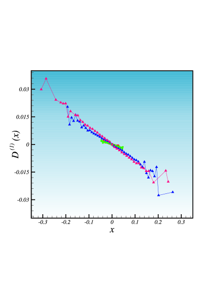
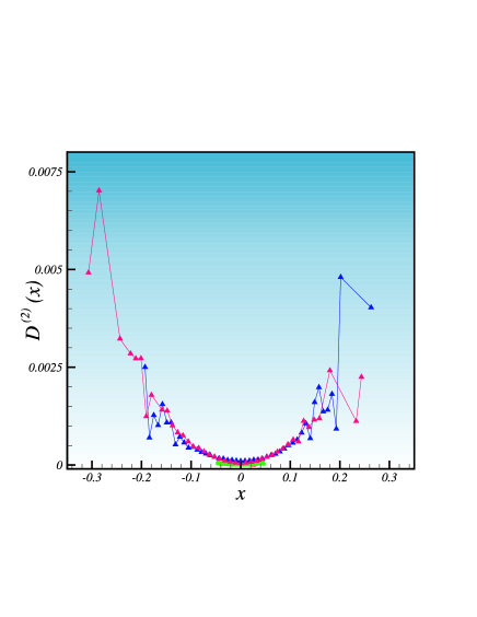
FIG. 5.: The drift and diffusion coefficients, $D^{(1)}(x)$ and $D^{(2)}(x)$, estimated by Eq. (18). For the healthy subjects (triangles) and for patients with CHF (squares), $D^{(1)}(x)$ and $D^{(2)}(x)$ follow linear and quadratic equations in $x$.

We distinguish the healthy subjects from those with CHF in terms of the differences between the drift and diffusion coefficients of the Fokker-Plank equations that we construct for the returns data which, in our view, provide a clearer and more physical way of understanding the differences between the two groups of the subjects. In addition, the reconstruction method suggested in this paper enables one to predict the future trends in the returns (and, hence, in the original series $r_{i}$) over time scales that are of the order of the Markov time scale $t_{M}$. None of the previous approaches for analyzing the data could provide such a reconstruction method.

We also believe that, the computational method that is described in this paper is more sensitive to small differences between the data for healthy subjects and those with CHF. As such, it might eventually provide a diagnostic tool for detection of CHF in patients with small amounts of data and in its initial stages of development.

REFERENCES

- [1] C.-K. Peng, J. Mietus, J. M. Hausdorff, S. Havlin, H. E. Stanley and A. L. Goldberger, Phys. Rev. Lett. 70, 1343 (1993)
- [2] A. Bunde, S. Havlin, J. W. Kantelhardt, T. Penzel, J.-H. Peter, and K. Voigt, Phys. Rev. Lett. 85, 3736 (2000).
- [3] P. Bernaola-Galvan, P. Ch. Ivanov, L. N. Amaral, and H. E. Stanley, Phys. Rev. Lett. 87, 168105 (2001)
- [4] V. Schulte-Frohlinde, Y. Ashkenanzy, P. Ch. Ivanov, L. Glass, A. L. Goldberger, and H. E. Stanley, Phys. Rev. Lett. 87, 068104 (2001)
- [5] Y. Ashkenazy, P. Ch. Ivanov, Shlomo Havlin, C-K. Peng, A. L. Goldberger, and H. E. Stanley, Phys. Rev. Lett. 86, 1900 (2001)
- [6] T. Kuusela, Phys. Rev. E 69, 031916 (2004).
- [7] S. Torquato, Random Heterogeneous Materials (Springer, New York, 2002); C.L.Y. Yeong and S. Torquato, Phys. Rev. E 57, 495 (1998); ibid. 58, 224 (1998).
- [8] M. Sahimi, Heterogeneous Materials, Volume II (Springer, New York, 2003).
- [9] G. R. Jafari, S. M. Fazlei, F. Ghasemi, S. M. Vaez Allaei, M. Reza Rahimi Tabar, A. Iraji Zad, and G. Kavei, Phys. Rev. Lett. 91, 226101 (2003).
- [10] M. Reza Rahimi Tabar, F. Ghasemi, J. Peinke, R. Friedrich, K. Kaviani, F. Taghavi, S. Sadeghi, G. Bijani and M. Sahimi,Computing In Scince and Engeering. ,86, (2006)
- [11] F. Ghasemi, J. Peinke, M. Sahimi, and M.R. Rahimi Tabar, European Physical J. B 47, 411 415, 29 (2005).
- [12] F. Ghasemi, J. Peinke M. Reza Rahimi Tabar and Muhammad Sahimi, to be published in Int l J. Modern Physics C, (2005).
- [13] R. Friedrich and J. Peinke, Phys. Rev. Lett. 78, 863 (1997).
- [14] J. Davoudi and M. Reza Rahimi Tabar, Phys. Rev. Lett. 82, 1680 (1999).
- [15] R. Friedrich, J. Peinke, and C. Renner, Phys. Rev. Lett. 84, 5224 (2000).
- [16] R. Friedrich, Th. Galla, A. Naert, J. Peinke and Th. Schimmel, in A Perspective Look at Nonlinear Media, edited by J. Parisi, S.C. Muller, and W. Zimmermann, Lecture Notes in Physics, 503 (Springer, Berlin, 1997), p. 313; R. Friedrich, S. Siegert, J. Peinke, et al., Phys. Lett. A 271, 217 (2000).
- [17] M. Siefert, A. Kittel, R. Friedrich, and J. Peinke, Euro. Phys. Lett. 61, 466 (2003); S. Kriso, et al., Phys. Lett. A 299, 287 (2002); S. Siegert, R. Friedrich, and J. Peinke, Phys. Lett. A 243, 275 (1998).
- [18] H. Risken, The Fokker-Planck Equation (Springer, Berlin, 1984).
- [19] M. M. Wolf, G. A. Varigos, D. Hunt, and J. G. Sloman, Med. J. Aust 2, 52 (1978).
- [20] P. Ch. Ivanov, A. Bunde, L. A. N. Amaral, S. Havlin, J. Fritsch-Yelle, R. M. Baevsky, H. E. Stanley, and A. L. Goldberger, Europhys. Lett. 48, 594 (1999).
- [21] P. Ch. Ivanov, L. A. N. Amaral, A. L. Goldberger, S. Havlin, M. G. Rosenblum, Z. Struzik, and H. E. Stanley, Nature (London) 399, 461 (1999).
- [22] C.-K. Peng, S. Havlin, H.E. Stanley, and A.L. Goldberger, Chaos 5, 82 (1995)
- [23] C.-K. Peng, S.V. Buldyrev, S. Havlin, M. Simons, H.E. Stanley, and A.L. Goldberger, Phys. Rev. E 49, 1685 (1994).
- [24] P.Ch. Ivanov, L.A.N. Amaral, A.L. Goldberger, and H.E. Stanley, Europhys. Lett. 43, 363 (1998).
- [25] R.G. Turcott and M.C. Teich, Ann. Biomed. Eng. 24, 269 (1996).
- [26] L.A. Lipsitz, J. Mietus, G.B. Moody, and A.L. Goldberger, Circulation 81, 1803 (1990).
- [27] D.T. Kaplan,et al,Biophys. J. 59, 945 (1991).
- [28] N. Iyengar, et al., Am. J. Physiol. 271, R1078 (1996).
- [29] C.-K.Peng, J.M. Hausdorff, and A.L. Goldberger,Nonlinear Dynamics, Self-Organization, and Biomedicine, edited by J. Walleczek, Cambridge University Press, Cambridge (1999).
- [30] D.C. Lin, Int. J. Mod. Phys. C 16, 465 (2005).
- [31] E.A. Novikov, Dokl. Akad. Nauk USSR 168, 1279 (1966).
- [32] D. Sornette, Phys. Rep. 297, 239 (1998).
- [33] A. Johansen, D. Sornette, and O. Ledoit, it J. Risk 1, 5 (1999).
- [34] W.-X. Zhou and D. Sornette, Physica D 165, 94 (2002).
- [35] D. Sornette and C.G. Sammis, J. Phys. I France 5, 607 (1995).
- [36] D. Stauffer and D. Sornette, Physica A 252, 271 (1998).
- [37] M. Saadatfar and M. Sahimi, Phys. Rev. E. 65, 036116 (2002).
- [38] M. Sahimi and S. Arbabi, Phys. Rev. Lett. 77, 3689 (1996).