Finite driving rate and anisotropy effects in landslide modeling

Abstract

In order to characterize landslide frequency-size distributions and individuate hazard scenarios and their possible precursors, we investigate a cellular automaton where the effects of a finite driving rate and the anisotropy are taken into account. The model is able to reproduce observed features of landslide events, such as power-law distributions, as experimentally reported. We analyze the key role of the driving rate and show that, as it is increased, a crossover from power-law to non power-law behaviors occurs. Finally, a systematic investigation of the model on varying its anisotropy factors is performed and the full diagram of its dynamical behaviors is presented.

I Introduction

Over the last two decades, the evidence of power laws in frequency-size distributions of several natural hazards such as earthquakes ofc , volcanic eruptions simkin , forest fires ff ; ff2 ; colloquium and landslides colloquium ; dussauge03 has suggested a relationship between these complex phenomena and self-organized criticality (SOC) bak96 . The idea of SOC bak87 , applied to many media exhibiting avalanche dynamics jensen98 ; turcotte99 , refers to the tendency of natural systems to self-organize into a critical state where the distribution of event sizes is represented by a power law with an exponent $\alpha$, which is universal in the sense that it is robust to minor changes in the system. Generally, the nature of a critical state is evidenced by the fact that the size of a disturbance to the system is a poor predictor of the system response. Let us consider storms as perturbations for natural slopes. Large storms can produce large avalanches, but also small storms sometimes can do it. On the other hand, small storms usually do not produce any avalanche, but also large storms may not cause any avalanching phenomena. Moreover, avalanches triggered by small storms can be larger than those triggered by large storms. The unpredictability of the sizes of such system responses to incremental perturbations and the observed power-law statistics could be the exhibition of self-organized critical behavior in most natural avalanches. However, the idea of understanding power-law distributions within the framework of SOC is not the only one. Recently, in order to reproduce the range of the power-law exponents observed for landslides, some authors have introduced a two-threshold cellular automaton, which relates landslide dynamics to the vicinity of a breakdown point rather than to self-organization faillettaz .

In this paper, we report an accurate investigation of a cellular automaton model, which we have recently proposed to describe landslide events and, specifically, their frequency-size distributions grl . In particular, we discuss the role of a finite driving rate and the anisotropy effects in our non-conservative system. It has been pointed out by several authors that the driving rate is a parameter that has to be fine tuned to zero in order to observe criticality sornette ; vespignani ; HNJ . We notice that the limit of zero driving rate is only attainable in an ideal chain reaction, therefore finite rates of external drives are essential ingredients in the analysis of the dynamics of real avalanche processes. We show that increasing the driving rate the frequency-size distribution of landslide events evolves continuously from a power-law (small driving rates) to an exponential (Gaussian) function (large driving rates). Interestingly, a crossover regime characterized by a maximum of the distribution at small sizes and a power-law decay at medium and large sizes is found in the intermediate range of values of the driving rate for a wide range of level of conservation. Power-law behaviors are robust even though their exponents depend on the system parameters (e.g., driving rate and level of conservation, see below).

Although the critical nature of landslides is not fully assessed and many authors believe that deviations from power law appear to be systematic for small landslides data brardinoni ; malamud04 , results from several regional landslide inventories show robust power-law distributions of medium and large events with a critical exponent $\alpha\sim 2.5\pm 0.5$ dussauge03 . The variation in the exponents of landslide size distributions is larger than in the other natural hazards that exhibit scale-invariant size statistics hergarten03 . Whether this variation of $\alpha$ is caused by scatter in the data or because different exponents are associated with different geology, is an important open question, which we may contribute to address.

The model we analyze describes the evolution of a space and time dependent factor of safety field. The factor of safety ($FS$) is defined as the ratio between resisting forces and driving forces. It is a complicate function of many dynamical variables (pore water pressure, lithostatic stress, cohesion coefficients, etc.) whose rate of change is crucial in the characterization of landslide events. A landslide event may include a single landslide or many thousands. We investigate frequency-size distributions of landslide events by varying the driving rate of the factor of safety. Although our probability density distributions are lacking of a direct comparison with frequency-size distributions of real landslides they reproduce power-law scaling with an exponent very close to the observed values. Moreover, they allow us to get insight into the difficult problem of the determination of possible precursors of future events.

The paper is organized as follows. In the next Section, we present the model and briefly discuss the differences between our approach and previous cellular automata models that have been recently introduced to characterize landslide frequency-size distributions. In Section III, we report numerical results obtained by a systematic investigation of the effects of a finite driving rate on the frequency-size distribution. The values of the exponent of the power-law decay are given as a function of the driving rate and the level of conservation. An accurate analysis of the spatial distribution of the values of the factor of safety by varying the driving rate provides useful information for quantifying hazard scenarios of possible avalanche events. In Section IV, we analyze the role of anisotropic transfer coefficients, which control the propagation of the instability. We summarize our results in a phase diagram that shows the location of power-law and non power-law scaling regions in the anisotropy parameter space. Conclusions are summarized in Section V.

II The Model

The instability in clays often starts from a small region, destabilizes the neighborhood and then propagates bjerrum . Such a progressive slope failure recalls the spreading of avalanches in the fundamental models of SOC. The term self-organized criticality (SOC) was coined by Bak, Tang and Wiesenfeld to describe the phenomenon observed in a particular cellular automaton model, nowadays known as the sandpile model bak87 . In the original sandpile model, the system is perturbed externally by a random addition of sand grains. Once the slope between two contiguous cells has reached a threshold value, a fixed amount of sand is transferred to its neighbors generating a chain reaction or avalanche. The non-cumulative number of avalanches $N_{A}$ with area $A$ satisfies a power-law distribution with a critical exponent $\alpha=1$ kadanoff , which is much smaller than the values of the power-law exponents observed for landslides colloquium ; dussauge03 . Few years later the paper of Bak et al. bak87 , Olami, Feder and Christensen (OFC) recognized the dynamics of earthquakes as a physical realization of self-organized criticality and introduced a cellular automaton that gives a good prediction of the Gutenberg-Richter law ofc . Such a model, whose physical background belongs to the Burridge-Knopoff spring-block model bk , is based on a continuous dynamical variable which increases uniformly through time till reaches a given threshold and relaxes. This means that the dynamical variable decreases, while a part of the loss is transferred to the nearest neighbors. If this transfer causes one of the neighbors to reach the threshold value, it relaxes too, resulting in a chain reaction. OFC recognized that the model still exhibits power-law scaling in the non-conservative regime, even if the power-law exponent strongly depends on the level of conservation.

In this paper, we investigate the role of a finite driving rate and of anisotropy in a non-conservative cellular automaton modeling landslides grl . In such a model, we sketch a natural slope by using a square grid where each site $i$ is characterized by a local value of the safety factor $FS_{i}$. In slope stability analysis, the factor of safety, $FS$, against slip is defined in terms of the ratio of the maximum shear strength $\tau_{max}$ to the disturbing shear stress $\tau$

$$FS=\frac{\tau_{max}}{\tau}.$$ (1)

The limited amount of stress that a site can support is given by the empirical Mohr-Coulomb failure criterion: $\tau_{max}=c+(\sigma-u)\tan\phi$, where $\sigma$ is the total normal stress, $u$ is the pore-fluid pressure, $\phi$ is the angle of internal friction of the soil and $c$ is the cohesional (non-frictional) component of the soil strength terzaghi . If $FS>1$, resisting forces exceed driving forces and the slope remains stable. Slope failure starts when $FS=1$. Since a natural slope is a complex non-homogeneous system characterized by the presence of composite diffusion, dissipative and driving mechanisms acting in the soil (such as those on the water content), we consider time and site dependent safety factor $FS_{i}$ and treat the local inverse factor of safety $e_{i}=1/FS_{i}$ as the non-conserved dynamical variable of our cellular automata model grl .

The long-term driving of the OFC model is, here, replaced by a dynamical rule which causes the increases of $e_{i}$ through the time with a finite driving rate $\nu$: $e_{i}(t+\Delta t)=e_{i}(t)+\nu\Delta t$. Such a rule allows us to simulate the effect on the factor of safety of different complex processes which can change the state of stress of a cell. The model is driven as long as $e_{i}<1$ on all sites $i$. Then, when a site, say $i$, becomes unstable (i.e., exceeds the threshold, $e_{th}=1$) it relaxes with its neighbors according to the rule:

$$e_{i}\rightarrow 0;\quad\quad e_{nn}\rightarrow e_{nn}+f_{nn}e_{i},$$ (2)

where $nn$ denotes the nearest neighbors of site $i$ and $f_{nn}$ is the fraction of $e_{i}$ toppling on $nn$. This relaxation rule is considered to be instantaneous compared to the time scale of the overall drive and lasts until all sites remain below the threshold. When $e_{i}$ reaches the threshold value $1$ and relaxes, the fraction of $e_{i}$ moving from the site $i$ to its “downward” (resp. “upward”) neighbor on the square grid is $f_{d}$ (resp. $f_{u}$), as $f_{l}=f_{r}$ is the fraction to each of its “left” and “right” neighbors. The transfer parameters $f_{nn}$ are chosen in order to individuate a privileged transfer direction: we assume $f_{u}<f_{d}$ and $f_{l}=f_{r}<f_{d}$. We notice that the model reproduces features of the OFC model for earthquakes in the limit case $\nu=0$ and $f_{nn}=f\leq 0.25$. A detailed analysis of the model on varying the transfer coefficients $f_{nn}$ is reported in Sec. IV.

Since many complex dissipative phenomena (such as evaporation mechanism, volume contractions, etc. fredlund ) contribute to a dissipative stress transfer in gravity-driven failures, we study the model in the non-conservative case $C=\sum_{nn}f_{nn}<1$, which makes our approach different from previous ones within the framework of SOC hergarten03 . The conservation level, $C$, and the anisotropy factors, which we consider here to be uniform, are actually related to local soil properties (e.g., lithostatic, frictional and cohesional properties), as well as to the local geometry of the slope (e.g., its morphology). The rate of change of the inverse factor of safety, $\nu$, induced by the external drive (e.g., rainfall), in turn related to soil and slope properties, quantifies how the triggering mechanisms affect the time derivative of the FS field.

Recently, in order to reproduce the range of the power-law exponents observed for landslides, several authors have used two-threshold cellular automata, which relate landslide dynamics to self-organization hergarten00 or to the vicinity of a breakdown point faillettaz . In the first approach hergarten00 , a time-dependent criterion for stability, with a not easy interpretation in terms of governing physics, provides a power-law exponent close to 2 without any tuning. Therefore, this approach does not explain the observed variability of $\alpha$. In Ref. faillettaz , the range of $\alpha$ is found by tuning the maximum value of the ratio between the thresholds of two failure modes, the shear failure and the slab failure. However, the frequency-size distribution of avalanches is obtained by counting only clusters where shear failures have occurred, considering conservative transfer processes between adjacent cells with a different number of nearest neighbors. In this paper, the investigation of our non-conservative cellular automaton is mainly devoted to the characterization of landslide event dynamics on varying the driving rate in order to analyze different hazard scenarios.

III The effect of a finite drive on frequency-size distributions

Figure 1: Noncumulative frequency-size distributions on a $64\times 64$ grid corresponding to four values of the driving rate. The logarithm of the normalized number of model events, $log_{10}[P(s)]$, in which a specified number of different cells, $s$, become unstable, is given as a function of $log_{10}(s)$. We show the case $C=0.4$, $f_{u}/f_{d}=2/3$ and $f_{l}/f_{d}=5/6$.

Frequency-size distributions give the number of landslides (events) as a function of their size. In Fig.1 we show the non-cumulative frequency-size distributions obtained for different values of the driving rate in the anisotropic non conservative case $C=0.4$, with $f_{u}/f_{d}=2/3$ and $f_{l}/f_{d}=5/6$. The curves are obtained for a square lattice of size $64\times 64$. We considered both cylindrical (open along the vertical axis and periodical along the horizontal axis) and open boundary conditions, which we checked differ in the slopes of the distribution curves for less than $1\%$.

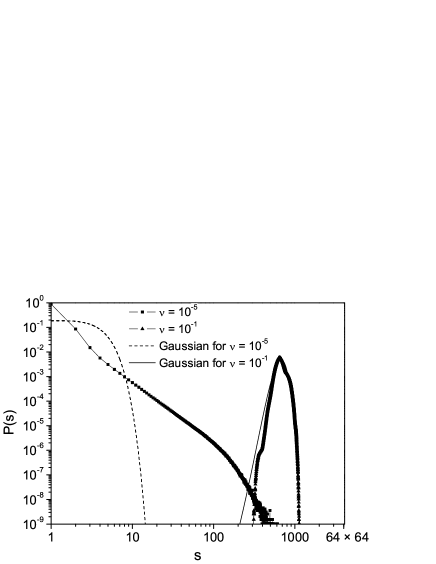
Figure 2: Noncumulative frequency-size distributions and corresponding Gaussian distributions on a $64\times 64$ grid for two values of the driving rate. Squares and triangles show the normalized number of model events, $P(s)$, in which a specified number of different cells, $s$, become unstable as a function of $s$. The dashed and the solid lines are Gaussian distributions obtained for the same mean value and the standard deviation of the frequency-size distributions. We consider the case $C=0.4$, $f_{u}/f_{d}=2/3$ and $f_{l}/f_{d}=5/6$.

In the limit of vanishing driving rate, the distribution of events, $P(s)$, is similar to that of the two-dimensional isotropic OFC model for a fixed value of the level of conservation: a power law characterized by a critical exponent $\alpha$, $P(s)\sim s^{-\alpha}$, followed by a system finite-size dependent exponential cutoff jensen98 . As discussed in Ref. grl , by increasing the driving rate $\nu$, the probability distribution develops a maximum, which shifts towards larger events with $\nu$. On the left side of the maximum, a power-law decay, with exponent $\beta$ (see the Fig. 1), seems to appear for small landslide sizes. However, the few available data do not allow to distinguish log-log linear shape and an exponential one malamud04 . On the right side of the maximum of the distribution, the power-law regime remains until, by increasing $\nu$, the distribution continuously modifies in a bell-shaped curve. Fig.2 shows the crossover of the probability distribution from power-law to Gaussian on increasing the driving rate.

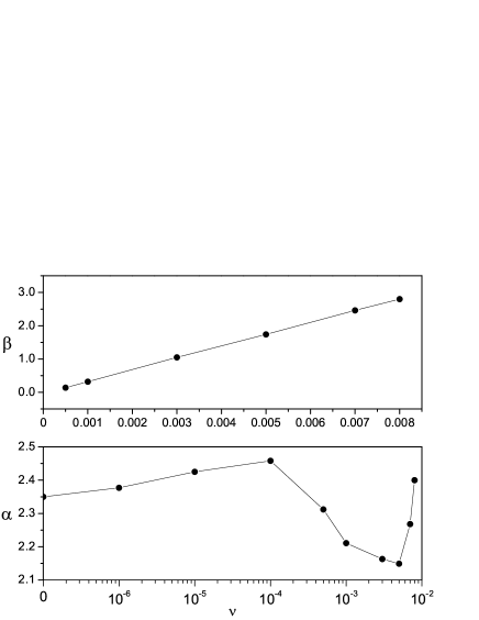
Figure 3: Top: Positive power-law exponent $\beta$ as a function of the driving rate $\nu$. Bottom: Negative power-law exponent $\alpha$ as a function of $\nu$. The values of the exponents are obtained for $C=0.4$, $f_{u}/f_{d}=2/3$ and $f_{l}/f_{d}=5/6$.

Figure 4: Top: Positive power-law exponent $\beta$ as a function of the level of conservation $C$. Bottom: Negative power-law exponent $\alpha$ as a function of $C$. The values of the exponents are obtained for $\nu=0.003$, $f_{u}/f_{d}=2/3$ and $f_{l}/f_{d}=5/6$.

The behavior of the power-law exponents on varying $\nu$ is shown in Fig.3. Interestingly, the values of the power-law exponent $\alpha$ are very close to those experimentally reported colloquium . As one can see, $\alpha$ increases until the value of the driving rate sensitively modifies the shape of the distribution with the appearance of a maximum. We find that the regime with a non-monotonic frequency-size distribution is robust to changes in system parameters. In particular, it can be found for $\nu\in[10^{-4},10^{-2}]$ in the whole range $C\in[0.4,0.8]$.

The values of the exponents $\alpha$ and $\beta$ sensitively change by varying another important parameter of the model that is the level of conservation $C$, which represents the non-conservative redistribution of the load of failing cells. The effect of $C$ at finite driving rate is comparable to that obtained at $\nu=0$ ofc , as shown in Fig.4 (see also Ref. grl ).

Figure 5: Size, $s$, of equiprobable events (i.e., corresponding to the same probability of occurrence) as a function of the driving rate. Top: Sizes of model events with $P(s)=10^{-2}$. Bottom: Sizes of model events with $P(s)=10^{-6}$. In the top panel, only the largest sizes of equiprobable events are plotted.

Figure 6: (top row) Snapshots of a landslide event of size $s=230$ on a $64\times 64$ grid, for four values of the driving rate (from left to right): $\nu=10^{-5}$, $\nu=10^{-3}$, $\nu=5\cdot 10^{-3}$ and $\nu=5\cdot 10^{-2}$. The 230 black cells are those that have reached the instability threshold. The simulations are done in the case $C=0.4$, $f_{u}/f_{d}=2/3$ and $f_{l}/f_{d}=5/6$. (bottom row) Snapshots of the factor of safety corresponding to the stable configurations reached after the avalanches shown in top row. The values of the factor of safety have been associated to ten levels of a gray scale from white to black, in order to measure the distance of a cell from its instability condition: the darker the color, the farther is the cell from the instability threshold.

Let us come back to Fig.1 in order to highlight the role of the driving rate in the characterization of landslide events. From the distributions of Fig.1, we see that large events can have comparatively high probabilities in the power-law regime (i.e., at small driving rates $\nu$) with respect to the Gaussian regime (i.e., larger $\nu$). Such a feature could allow to reproduce the observation that sometimes mild rainfalls produce landslides as large as those triggered by intense rainfalls. To underline the nonlinear behavior of the system with $\nu$, in Fig.5 we plot the sizes of avalanches with the same probability of occurrence for different values of the driving rate. Such sizes are the intersections of horizontal straight lines with the distribution curves of Fig.1. When we consider small events (i.e., $P(s)$ as large as $10^{-2}$), we find that the size of equiprobable events increases with the driving rate. Thus, for equiprobable events with high probability of occurrence the system response is essentially linear with the driving rate. Instead, for large events (i.e., $P(s)$ as small as $10^{-6}$), the size of equiprobable events has a maximum as a function of $\nu$. Thus, it appears that, for a given range of $\nu$ values, the size of events caused by a slow rate of changes of the factor of safety can be larger than the size of avalanches triggered by a faster rate. Moreover, an evidence is found for the existence of the most dangerous value of $\nu$, for which the size of the system response has a maximum.

III.1 Hazards scenarios

The detection of possible precursors of a landslide event is a crucial step to achieve hazard reduction. In order to get insight into this difficult problem, we visualize the structure of a typical landslide event for different values of the driving rate $\nu$. In the top row of Fig.6, we report on the $64\times 64$ grid a typical avalanche of size $s=230$ on increasing the value of $\nu$ from left to right. The $230$ black cells are those that have reached the instability threshold. As we can see, compact landslides are the characteristic response of a system governed by power-law statistics as it happens at small $\nu$ (also when a maximum in the frequency-size distribution develops). Such a response is typical of systems with SOC behavior pietronero . By increasing the driving rate, compact clusters survive until power-law regime disappears. As the system enters the non power-law regime, the relevance of domino effects drastically drops and landslide events are characterized by many tiny independent clusters.

In the bottom row of Fig.6, we show the distribution of the factor of safety $FS_{i}=1/e_{i}$ for the cases corresponding to the upper panels nota1 . The distribution on the grid of the values shows how the spatial correlations in the system crucially affect landslide structures. In order to measure the distance of a cell from its instability condition and to visualize the correlated areas (regions with similar values of $FS_{i}$), the values of $FS_{i}$ have been associated to ten levels of a gray scale from white to black: the darker the color, the farther is the cell from the instability threshold. In the snapshots of Fig.6, it is possible to recognize as dark areas the avalanches shown in the corresponding upper grids. In particular, the dark areas typically are related to previous landslide events, whereas the lighter areas indicate regions of future events. We notice that in the power law regime (i.e. small $\nu$) even a very small perturbation (say, a drop of water) at one single point can trigger huge system responses. Instead, in the non power-law regime (i.e. large $\nu$) large-scale correlations are absent; here large events trivially occur just because the strong external driving rate makes likely that many cells simultaneously approach the instability threshold. Thus, the detection of patterns of correlated domains in investigated areas results to be a crucial tool to identify the response of the system to perturbations, i.e., to hazard assessment.

It is worth noticing that the average value of the factor of safety on the grid cells $<FS>$ and its fluctuation $<\Delta FS^{2}>$ are very similar in the four cases showed in Fig.6, encompassing a broad spectrum of $\nu$ values. Interestingly, the probability distribution of $FS$ on the grid sites, independently of the driving rate, is well approximated by a Gaussian distribution. This suggests that a measure of just an average safety factor on the investigated area could provide only a very partial information about the statistics governing the considered landslide events.

IV Anisotropy effects on frequency-size distributions

In the previous sections, we have investigated the properties of the model on varying the driving rate $\nu$ at fixed values of the anisotropic ratios $f_{u}/f_{d}$ and $f_{l}/f_{d}=f_{r}/f_{d}$. Such parameters control how the instability propagates downward and, therefore, they are complicate functions of the topography and geology of a specific area. In this Section, we are interested in the analysis of the model when such transfer coefficients vary.

It is well-known that the one-dimensional version of the sandpile and OFC models are characterized by non power-law scaling jensen98 . Thus, we expect that, for small values of the ratio $f_{l}/f_{d}$, the frequency-size distribution does not show power-law behavior. Viceversa, for $f_{u}/f_{d}\sim 1$ and $f_{l}/f_{d}\sim 1$, we expect to have power-law distributions, as in the OFC model, which corresponds in our model to the limit $f=f_{u}=f_{l}=f_{r}=f_{d}$ and $\nu=0$.

The diagram of Fig.7 summarizes the different regimes found in our simulations at fixed values of the driving rate $\nu=10^{-4}$ and the level of conservation $C=0.4$. We find that, on varying the anisotropic ratios, the parameter space is divided in three regions: i) a power-law region (PL) characterized by power-law frequency-size distributions for large values of the anisotropic ratios, ii) a non power-law region (NPL) for the whole range of values of the anisotropic ratio $f_{u}/f_{d}$ (which controls the redistribution of load in the vertical direction) and small values of $f_{l}/f_{d}$, iii) a finite-size oscillation region (FSO) where the frequency-size distribution is characterized by periodic peaks, which appear for integer multiples of the grid size $L=64$.

Figure 7: Phase diagram in the $f_{u}/f_{d}$ vs. $f_{l}/f_{d}$ plane. The lines divide the parameter space in three regions: a power-law scaling region (PL), a non power-law scaling region (NPL) and a finite-size oscillation region (FSO) where peaks of the distribution commensurate with the size of the grid appear. The results are obtained for $\nu=10^{-4}$ and $C=0.4$.

As expected, we find power-law and non power-law behaviors for large and small values of the anisotropic ratios, respectively. In particular, we find that the value of the critical exponent $\alpha$ of the power-law distribution slightly increases with $f_{u}/f_{d}$ for a fixed value of $f_{l}/f_{d}$ and decreases with $f_{l}/f_{d}$ for a fixed value of $f_{u}/f_{d}$. However, the changes in $\alpha$ are negligible.

It is worth noticing that, even if the ratio $f_{l}/f_{d}$ is quite large, we find that the frequency-size distribution does not show a power law decay when the value of $f_{u}/f_{d}$ is small, (see Fig.7). Indeed, the probability distribution develops a finite number of peaks which are commensurate with the size of the grid. Fig.8 shows the frequency-size distribution for two different values of the anisotropic ratios in the FSO region of the phase diagram. By increasing $f_{l}/f_{d}$, the peaks of the distributions turn down as long as they disappear. We m that several peaks in the distribution of avalanche sizes are obtained in Ref. corral . The authors vary the convexity of the driving $\gamma$ and the level of conservation $\epsilon$ in the isotropic case: $C=1$ when $\epsilon=0.25$. They find an intermediate region of the phase-diagram $\epsilon$ vs. $\gamma$ where the frequency-size distribution is characterized by peaks that scale with different powers of the system size $L$. Fixing the convexity of the driving $\gamma$ ($\gamma=0$ for a uniform driving), for large values of the level of conservation, $C\geq 0.6$, the peaks disappear and they get a power-law decay with an exponential cutoff. Conversely, we find commensurate peaks in the FSO region in the whole range $C\in[0.4,0.8]$.

Figure 8: Noncumulative frequency-size distributions on a $64\times 64$ grid for $f_{u}/f_{d}=0$ and $f_{l}/f_{d}=0.3$ (triangles) and $f_{l}/f_{d}=0.55$ (squares). The inset shows the distribution curves in a log-linear scale for the range of values where commensurate peaks are observed. The vertical lines mark multiples of the system size. The results are obtained for $\nu=10^{-4}$ and $C=0.4$.

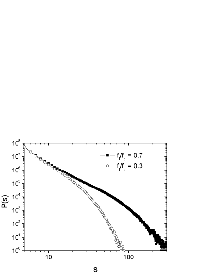
Figure 9: Noncumulative frequency-size distributions on a $64\times 64$ grid for $f_{u}/f_{d}=1$ and $f_{l}/f_{d}=0.3$ (open dots) and $f_{l}/f_{d}=0.7$ (squares). The results are obtained for $\nu=10^{-4}$ and $C=0.4$.

We notice that an analysis of the anisotropic case of the OFC model is made in Ref.christensen92 where the authors introduce only two transfer coefficients $\alpha_{1}=f_{l}=f_{r}$ and $\alpha_{2}=f_{u}=f_{d}$ and control the degree of anisotropy by changing the ratio $\alpha_{1}/\alpha_{2}$, while keeping the level of conservation constant. They find that the anisotropy has almost no effect on the power-law exponent while the scaling exponent, expressing how the finite-size cutoff scales with the system size, changes continuously from a two-dimensional to a one dimensional scaling of the avalanches christensen92 . Varying the anisotropic ratio $\alpha_{1}/\alpha_{2}$ in the range $[0,1]$ is equivalent to consider the straight line $f_{u}/f_{d}=1$ in the phase diagram of Fig.7. As in Ref. christensen92 , we find that on moving along the line $f_{u}/f_{d}=1$, the changes in the power-law exponent are negligible. However, differently Ref. christensen92 , we find a crossover in the frequency-size distribution behavior from power-law to non power-law (see Fig. 9). We attribute such a different result to the finite driving rate.

In conclusion, our analysis shows that only a finite range of values of the anisotropic transfer coefficients can supply power-law distributions. This characterization provides insight into the difficult determination of the complex and non-linear transfer processes that occur in a landslide event.

V Concluding Remarks

Explanation of the power-law statistics for landslides is a major challenge, both from a theoretical point of view as well as for hazard assessment. In order to characterize frequency-size distributions of landslide events, we have investigated a continuously driven anisotropic cellular automaton based on a dissipative factor of safety field. We have found that the value of the driving rate, which describes the variation rate of the factor of safety due to external perturbations, has a crucial role in determining landslide statistics. In particular, we have shown that, as the driving rate increases, the frequency-size distribution continuously changes from power-law to gaussian shapes, offering the possibility to explain the observed rollover of the data for small landslides. The values of the calculated power-law exponents are in good agreement with the observed values. Moreover, the analysis of the model on varying the driving rate suggests the determination of correlated spatial domains of the factor of safety as a useful tool to quantify the severity of future landslide events.

As concerns the effects of anisotropic transfer coefficients, which control the non-conservative redistribution of the load of failing cells, we have found that the power-law behavior of the frequency-size distribution is a feature of the model only in a limited region of the anisotropy parameter space.

- (1) Z. Olami, H. J. S. Feder, K. Christensen, Phys. Rev. Lett. 68, 1244 (1992).
- (2) T. Simkin, Annu. Rev. Earth Planet. Sci. 21, 427 (1993).
- (3) P. Bak, K. Chen, C. Tang, Phys. Lett. A. 147, 297 (1992).
- (4) R. Pastor-Satorras, and A. Vespignani, Phys. Rev. E 61, 4854 (2000).
- (5) D. L. Turcotte, B. D. Malamud, F. Guzzetti, P. Reichenbach, Proc. Natl. Acad. Sci. U.S.A. 99, 2530 (2002).
- (6) C. Dussauge, J.R. Grasso, and A Helmstetter, J. Geophys. Res. 108, 2286 (2003).
- (7) P. Bak, How Nature Works - The Science of Self-Organized Criticality, (Copernicus, Springer-Verlag, New York, 1996).
- (8) P. Bak, C. Tang and K. Wiesenfeld, Phys. Rev. Lett. 59, 381 (1987); Phys. Rev. A 38, 364 (1988).
- (9) H. J. Jensen, “Self-Organized Criticality: emergent complex behavior in physical and biological systems” (Cambridge University Press, Cambridge, 1998).
- (10) D. L. Turcotte, Rep. Prog. Phys. 62, 1377 (1999).
- (11) J. Failletaz, F. Louchet, J.R. Grasso, Phys. Rev. Lett. 93, 208001 (2004).
- (12) E. Piegari, V. Cataudella, R. Di Maio, L. Milano, M. Nicodemi, Geophys. Res. Lett. in press.
- (13) D. Hamon, M. Nicodemi and H.J. Jensen, Astronomy&Astrophysics 387, 326 (2002).
- (14) R. Dickman, A. Vespignani, S. Zapperi, Phys. Rev. E 57, 5095 (1998).
- (15) D. Sornette, Critical Phenomena in Natural Sciences, Chaos, Fractals, Self-organization and Disorder: Concepts and Tools, (Springer Series in Synergetics, Heidelberg, 2004).
- (16) F. Brardinoni, M. Church, Earth Surf. Process. Landforms 29, 115 (2004).
- (17) B. D. Malamud, D. L. Turcotte, F. Guzzetti, P. Reichenbach, Earth Surf. Process. Landforms 29, 687 (2004).
- (18) S. Hergarten, Natural Hazards and Earth System Sciences 3, 505 (2003).
- (19) L. Bjerrum, J. Soil Mech. Fdns. Div. Am. Soc. Civ. Engnrs. 93, 3 1967.
- (20) L. P. Kadanoff, S. R. Nagel, L. Wu, S. M. Zhou, Phys. Rev. A 39, 6524 (1989).
- (21) R. Burridge and L. Knopoff, Bull. Seismol. Soc. Am. 57, 341 (1967).
- (22) K. Terzaghi, Geothecnique 12, 251 (1962).
- (23) D. G. Fredlund, H. Rahardjo, “Soil Mechanics for Unsatured Soils” (Wiley-Interscience, New York, 1993).
- (24) S. Hertgarten and H. J. Neugebauer, Phys. Rev. E 61, 2382 (2000).
- (25) In order to visualize the distribution, we introduced a lower threshold and checked that the results do not change.
- (26) L. Pietronero, W. R. Schneider, Phys. Rev. Lett. 66, 2336 (1991).
- (27) K. Christensen and Z. Olami, Phys. Rev. A 46, 1829 (1992)
- (28) A. Corral, C. J. Perez, A. Diaz-Guilera, A. Arenas, Phys. Rev. Lett. 74, 118 (1995)