Davies ENDOR revisited:
Enhanced sensitivity and nuclear spin relaxation

Abstract

Over the past 50 years, electron-nuclear double resonance (ENDOR) has become a fairly ubiquitous spectroscopic technique, allowing the study of spin transitions for nuclei which are coupled to electron spins. However, the low spin number sensitivity of the technique continues to pose serious limitations. Here we demonstrate that signal intensity in a pulsed Davies ENDOR experiment depends strongly on the nuclear relaxation time T_1n, and can be severely reduced for long T_1n. We suggest a development of the original Davies ENDOR sequence that overcomes this limitation, thus offering dramatically enhanced signal intensity and spectral resolution. Finally, we observe that the sensitivity of the original Davies method to T_1n can be exploited to measure nuclear relaxation, as we demonstrate for phosphorous donors in silicon and for endohedral fullerenes N@C₆₀ in CS₂.

I Introduction

Electron-nuclear double resonance (ENDOR) belongs to a powerful family of polarization transfer spectroscopic methods and permits the measurement of small energy (nuclear spin) transitions at the much enhanced sensitivity of higher energy (electron spin) transitions Feher (1956). ENDOR is thus an alternative to NMR methods, with the benefits of improved spin-number sensitivity and a specific focus on NMR transitions of nuclei coupled to paramagnetic species (reviewed in Refs Kevan and Kispert (1976); Schweiger and Jeschke (2001)).

In an ENDOR experiment, the intensity of an electron paramagnetic resonance (EPR) signal (e.g. an absorption signal in continuous wave EPR, or a spin echo signal in pulsed EPR) is monitored while strong RF irradiation is applied to excite nuclear spin transitions of the nuclei that are coupled to the electron spin. Although the EPR signal may be strong, the RF-induced changes are often rather weak and therefore it is quite common to find the ENDOR signal to constitute only a few percent of the total EPR signal intensity. Many different ENDOR schemes have been developed to improve sensitivity and spectral resolution of the ENDOR signal and to aid in analysis of congested ENDOR spectra Kevan and Kispert (1976); Schweiger and Jeschke (2001); Gemperle and Schweiger (1991). However, low visibility of the ENDOR signal remains a common problem to all known ENDOR schemes, and long signal averaging (e.g. hours to days) is often required to observe the ENDOR spectrum at adequate spectral signal/noise.

A low efficiency in spin polarization transfer (and thus low intensity of the ENDOR response) is inherent to continuous wave ENDOR experiments, which depend critically on accurate balancing of the microwave and RF powers applied to saturate the electron and nuclear spin transitions, and various spin relaxation times within the coupled electron-nuclear spin system, including the electron and nuclear spin-lattice relaxation times, T_1e and T_1n, and also the cross-relaxation (flip-flop) times, T_1x Dalton and Kwiram (1972). The ENDOR signal is measured as a partial de-saturation of the saturated EPR signal and generally constitutes a small fraction of the full EPR signal intensity Kevan and Kispert (1976). Since spin relaxation times are highly temperature dependent, balancing these factors to obtain a maximal ENDOR response is usually only possible within a narrow temperature range.

Pulsed ENDOR provides many improvements over the continuous wave ENDOR methods Gemperle and Schweiger (1991); Schweiger and Jeschke (2001) and most importantly eliminates the dependence on spin relaxation effects by performing the experiment on a time scale which is short compared to the spin relaxation times. Furthermore, combining microwave and RF pulses enables 100$\%$ transfer of spin polarization, and therefore the pulsed ENDOR response can in principle approach a 100$\%$ visibility (we define the ENDOR visibility as change in the echo signal intensity induced by the RF pulse, normalized to the echo intensity in the absence of the pulse Schweiger and Jeschke (2001); Epel et al. (2001)). In practice, the situation is far from perfect and it is common to observe a pulsed ENDOR response of the level of a few percent, comparable to continuous wave ENDOR. In this paper we discuss the limitations of the pulsed ENDOR method, and specifically Davies ENDOR Davies (1974). We suggest a modification to the pulse sequence which dramatically enhances the signal/noise and can also improve spectral resolution. We also show how traditional Davies ENDOR may be used to perform a measurement of the nuclear relaxation time, T_1n. While not discussed in this manuscript, a similar modification is also applicable to Mims ENDOR method Mims (1965).

II Materials and Methods

We demonstrate the new ENDOR techniques using two samples: phosphorus ³¹P donors in silicon, and endohedral fullerenes ¹⁴N@C₆₀ (also known as i-NC₆₀) in CS₂ solvent. Silicon samples were epitaxial layers of isotopically-purified ²⁸Si (a residual ²⁹Si concentration of $\sim 800$ ppm as determined by secondary ion mass spectrometry Itoh (2004)) grown on p-type natural silicon (Isonics). The epi-layers were 10 $\mu$m thick and doped with phosphorus at $1.6\cdot 10^{16}$ P/cm³. Thirteen silicon pieces (each of area 9$\times$3 mm²) were stacked together to form one EPR sample. This sample is referred as ²⁸Si:P in the text.

N@C₆₀ consists of an isolated nitrogen atom in the ⁴S_3/2 electronic state incarcerated in a C₆₀ fullerene cage. Our production and subsequent purification of N@C₆₀ is described elsewhere Kanai et al. (2004). High-purity N@C₆₀ powder was dissolved in CS₂ to a final concentration of 10¹⁵/cm³, freeze-pumped to remove oxygen, and finally sealed in a quartz tube. Samples were 0.7 cm long, and contained approximately $5\cdot 10^{13}$ N@C₆₀ molecules.

Both ²⁸Si:P and N@C₆₀ can be described by a similar isotropic spin Hamiltonian (in angular frequency units):

$$\mathcal{H}_{0}=\omega_{e}S_{z}-\omega_{I}I_{z}+a\!\cdot\!\vec{S}\!\cdot\!\vec{I},$$ (1)

where $\omega_{e}=g\beta B_{0}/\hbar$ and $\omega_{I}=g_{I}\beta_{n}B_{0}/\hbar$ are the electron and nuclear Zeeman frequencies, $g$ and $g_{I}$ are the electron and nuclear g-factors, $\beta$ and $\beta_{n}$ are the Bohr and nuclear magnetons, $\hbar$ is Planck’s constant and $B_{0}$ is the magnetic field applied along $z$-axis in the laboratory frame. In the case of ²⁸Si:P, the electron spin S=1/2 (g-factor = 1.9987) is coupled to the nuclear spin I=1/2 of ³¹P through a hyperfine coupling $a=117$ MHz (or 4.19 mT) Fletcher et al. (1954); Feher (1959). The X-band EPR signal of ²⁸Si:P consists of two lines (one for each nuclear spin projection $M_{I}=\pm 1/2$). Our ENDOR measurements were performed at the high-field line of the EPR doublet corresponding to $M_{I}=-1/2$. In the case of N@C₆₀, the electron has a high spin S=3/2 (g-factor = 2.0036) that is coupled to a nuclear spin I=1 of ¹⁴N through an isotropic hyperfine coupling $a=15.7$ MHz (or 0.56 mT) Murphy et al. (1996). The N@C₆₀ signal comprises three lines and our ENDOR experiments were performed on the central line ($M_{I}=0$) of the EPR triplet.

Pulsed EPR experiments were performed using an X-band Bruker EPR spectrometer (Elexsys 580) equipped with a low temperature helium-flow cryostat (Oxford CF935). The temperature was controlled with a precision greater than $0.05$ K using calibrated temperature sensors (Lakeshore Cernox CX-1050-SD) and an Oxford ITC503 temperature controller. This precision was needed because of the strong temperature dependence of the electron spin relaxation times in the silicon samples (T_1e varies by five orders of magnitude between 7 K and 20 K) Tyryshkin et al. (2003). Microwave pulses for $\pi$/2 and $\pi$ rotations of the electron spin were set to 32 and 64 ns for the ²⁸Si:P sample, and to 56 and 112 ns for the N@C₆₀ sample, respectively. In each case the excitation bandwidth of the microwave pulses was greater than the EPR spectral linewidth (e.g. 200 kHz for ²⁸Si:P Tyryshkin et al. (2003), and 8.4 kHz for N@C₆₀ Morton et al. (2005)) and therefore full excitation of the signal was achieved. RF pulses of 20-50 $\mu$s were used for $\pi$ rotations of the ³¹P nuclear spins in ²⁸Si:P and the ¹⁴N nuclear spins in N@C₆₀.

III Standard Davies ENDOR Sequence

Figure 1A shows a schematic of the Davies ENDOR sequence Davies (1974), while Figure 2A shows the evolution of the spin state populations during the sequence (for illustration purposes we consider a simple system of coupled electron S=1/2 and nuclear I=1/2 spins, however the same consideration is applicable to an arbitrary spin system). In the preparation step of the pulse sequence, a selective microwave $\pi$ pulse is applied to one of the electron spin transitions to transfer the initial thermal polarization (i) of the electron spin to the nuclear spin polarization (ii). In the mixing step a resonant RF pulse on the nuclear spin further disturbs the electron polarization to produce (iii), which can be detected using a two-pulse (Hahn) echo pulse sequence Schweiger and Jeschke (2001). A side result of the detection sequence is to equalize populations of the resonant electron spin states (iv). There then follows a delay, $t_{r}$, before the experiment is repeated (e.g. for signal averaging). Analysis of this recovery period has hitherto been limited (although the effect of $t_{r}$ has been discussed with respect to ENDOR lineshape Epel et al. (2001) and stochastic ENDOR acquisition Epel et al. (2003)), yet it is this recovery period which is crucial in optimizing the sequence sensitivity.

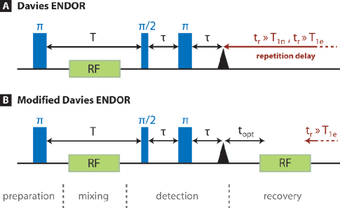
Figure 1: Pulse sequences for Davies ENDOR experiments. (A) The traditional Davies experiment requires long recovery time t${}_{r}\gg$ T_1e and t${}_{r}\gg$ T_1n to allow the spin system to fully recover to a thermal equilibrium before the experiment can be repeated (e.g. for signal averaging). (B) An additional RF pulse applied after echo detection helps the spin system to recover to a thermal equilibrium in a much shorter time limited only by T_1e. Thus, signal averaging can be performed at a much faster rate and an enhanced signal/noise can be achieved in a shorter experimental time. t_opt represents an optional delay of several T_1e which can be inserted for a secondary improvement in signal/noise and to avoid overlapping with electron spin coherences in case of long T_2e.

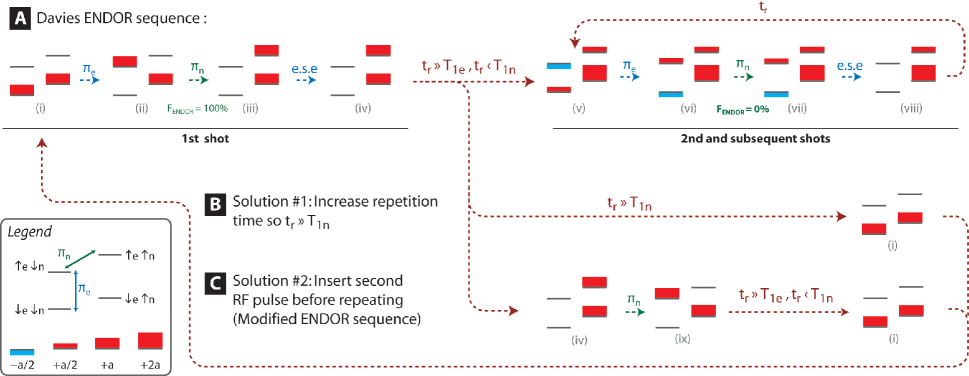
Figure 2: Evolution of spin state populations during the Davies ENDOR pulse sequence, for a coupled electron $S=1/2$ and nucleus $I=1/2$. Legend shows an energy level diagram and also electron ($\pi_{e}$) and nuclear ($\pi_{n}$) spin transitions excited by selective microwave and RF pulses, respectively. State populations are shown using colored bars (see legend) in a high-temperature approximation ($a=g\mu_{B}B/kT\ll 1$), ignoring the identity component and also the small thermal nuclear polarization. $g$ is the electron g factor, $\mu_{B}$ the Bohr magneton and $B$ the applied magnetic field. The ENDOR visibility, F_ENDOR, is measured as change in the electron spin polarization which occurs between (ii) and (iii), or (vi) and (vii), caused by the RF pulse. After the 2-pulse electron spin echo measurement (e.s.e.), there is a long delay, t_r, before the experiment is repeated. (A) In a typical experiment, T_1n,T${}_{1x}\gg$ t${}_{r}\gg$ T_1e, and so only the electron spin has time to relax — (iv) relaxes to (v), not to thermal equilibrium (i). The second and all subsequent experiments start from this new initial state (v). The RF pulse produces no changes to the state population, (vi) = (vii), and so the ENDOR signal is pessimal ($\sim 0\%$). (B) One solution is to increase the repetition time so that t${}_{r}\gg$ T_1n,T_1x, although this can lead to a very slow acquisition times. (C) A better solution is to apply an RF pulse ($\pi_{n}$) after the electron spin echo formation and detection. This additional RF pulse allows a faster return of the spin system to a thermal equilibrium, e.g. after several T_1e, irrespective of T_1n and T_1x.

Nuclear spin relaxation times T_1n (and also cross-relaxation times T_1x) are usually very long, ranging from many seconds to several hours, while electron spin relaxation times T_1e are much shorter, typically in the range of microseconds to milliseconds. In a typical EPR experiment, t_r is chosen to be several T_1e (i.e. long enough for the electron spin to fully relax, but short enough to perform the experiment in a reasonable time). Thus, in practice it is generally the case that T${}_{1n}\gg$ t${}_{r}\gg$ T_1e, i.e. t_r is short on the time scale of T_1n while long on the time scale of T_1e. With this choice of t_r, during the recovery period only the electron spin (and not the nuclear spin) has time to relax before the next experiment starts. As shown in Figure 2A, the second and all subsequent shots of the experiment will start from initial state (v), and not from the thermal equilibrium (i). While the first shot yields a 100$\%$ ENDOR visibility, subsequent passes give strongly suppressed ENDOR signals. Upon signal summation over a number of successive shots, the overall ENDOR response is strongly diminished from its maximal intensity and fails to achieve the theoretical 100$\%$ by a considerable margin.

One obvious solution to overcoming this limitation is to increase the delay time $t_{r}$ so that it is long compared to the nuclear spin relaxation time T_1n (Figure 2B). In other words, t${}_{r}\gg$ (T_1n, T_1x)$\gg$ T_1e, so that the entire spin system (including electron and nuclear spins) has sufficient time between successive experiments to fully relax to thermal equilibrium. However, this can make the duration of an experiment very long, and the advantage of an enhanced per-shot sensitivity becomes less significant. From calculations provided in the Appendix, it can be seen that an optimal trade-off between signal/noise and experimental time is found at t${}_{r}\approx 5/4$T_1n.

A better solution to this problem involves a modification of the original Davies ENDOR sequence which removes the requirement for t_r to be greater than T_1n, permitting enhanced signal/noise at much higher experimental repetition rates, limited only by T_1e.

IV Modified Davies ENDOR Sequence

Our modified Davies ENDOR sequence is shown in Figure 1B. An additional RF pulse is introduced at the end of the sequence, after echo signal formation and detection. This second RF pulse is applied at the same RF frequency as the first RF pulse and its sole purpose is to re-mix the spin state populations in such a way that the spin system relaxes to thermal equilibrium on the T_1e timescale, independent on T_1n. The effect of this second RF pulse is illustrated in Figure 2C. After echo signal detection, the spin system is in state (iv) and the second RF pulse converts it to (ix). This latter state then relaxes to thermal equilibrium (i) within a short t_r ($>3$T_1e). In this modified sequence each successive shot is identical and therefore adds the optimal ENDOR visibility to the accumulated signal.

The discussion in Figure 2C assumes an ideal $\pi$ rotation by the RF pulses. However, in experiment the RF pulse rotation angle may differ from $\pi$, and such an imperfection in either RF pulse will lead to a reduction in the ENDOR signal. Errors in the first pulse have the same effect as in a standard Davies ENDOR experiment, reducing the ENDOR signal by a factor $(1-\cos\theta)/2$, where $\theta$ the actual rotation angle. Errors in the second RF pulse (and also accumulated errors after the first pulse) cause incomplete recovery of spin system back to the thermal equilibrium state (i) at the end of each shot, thus reducing visibility of the ENDOR signal in the successive shots. The pulse rotation errors can arise from inhomogeneity of the RF field in the resonator cavity (e.g. spins in different parts of the sample are rotated by different angle) or from off-resonance excitation of the nuclear spins (when the excitation bandwidth of the RF pulses is small compared to total width of the inhomogeneously-broadened ENDOR line). It is desirable to eliminate (or at least partially compensate) some of these errors in experiment.

We find that introducing a delay t_opt, to allow the electron spin to fully relax before applying the second RF pulse (Figure 1B), helps to counter the effect of rotation errors. In numerical simulations, using the approach developed in ref. Epel et al. (2001); Bowman and Tyryshkin (2000) and taking into account electron and nuclear spin relaxation times and also a finite excitation bandwidth of the RF pulses, we observed that introducing t${}_{\rm{opt}}\gg T_{1e}$ produces about 30% increase in the ENDOR signal visibility (however, at cost of a slower acquisition rate with repetition time t${}_{\rm{opt}}+$ t_r). In the following sections, we demonstrate the capabilities of this modified Davies ENDOR sequence, using two examples of phosphorous donors in silicon and N@C₆₀ in CS₂.

V Application of the modified Davies ENDOR

V.1 Improved Sensitivity

Figure 3A shows the effect of experimental repetition time, t_r, on the ENDOR visibility, using a standard Davies ENDOR sequence applied to ²⁸Si:P. Although t_r is always longer than the electron spin relaxation time (T${}_{1e}=1$ ms for ²⁸Si:P at 10 K Tyryshkin et al. (2003)), increasing the repetition time from 13 ms to 1 second improves the visibility by an order of magnitude. As shown below, T${}_{1n}=288$ ms for the ³¹P nuclear spin at 10 K, and therefore we observe that the ENDOR signal visibility is weak ($\sim 2$%) when t${}_{r}=13$ ms is shorter than T_1n but the visibility increases to a maximum 22% when t${}_{r}=1$ s is longer than T_1n. The observed maximal visibility 22% does not reach a theoretical 100% limit because of the finite excitation bandwidth of the applied RF pulses ($t_{RF}=50$ $\mu$s in these experiments) which is smaller than total linewidth of the inhomogeneously-broadened ³¹P ENDOR peak.

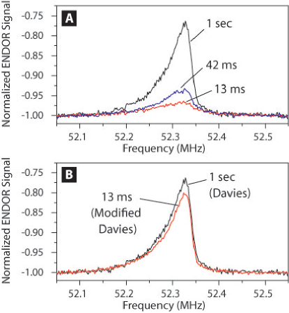
Figure 3: Davies ENDOR spectra for ²⁸Si:P, showing the low-frequency ³¹P nuclear transition line at 10 K. The spectra are normalized with respect to the spin echo intensity with no RF pulse applied. (A) Three spectra measured with the traditional Davies ENDOR pulse sequence (see Figure 1A) using different repetition times as labeled. The same number of averages (n=20) was applied for each spectrum and therefore the spectral acquisition times were approximately proportional to the repetition times (i.e. 5000, 210 and 65 seconds, respectively). (B) The spectrum measured with our modified Davies pulse sequence (see Figure 1B) using short repetition time (13 ms) shows a comparable signal/noise to the spectrum measured with a standard Davies pulse sequence at much longer repetition time (1 s). t_opt=6.5 ms was used in the modified Davies ENDOR experiment.

Through the use of the modified Davies ENDOR sequence proposed above, the same order of signal enhancement is possible at the faster 13 ms repetition time (e.g. at t${}_{r}\ll$ T_1n), as shown in Figure 3B. This is an impressive improvement indeed, considering that the acquisition time was almost 100 times shorter in the modified Davies ENDOR experiment. The signal is slightly smaller in the modified Davies ENDOR spectrum because of the imperfect $\pi$ rotation of the recovery RF pulse (e.g. due to inhomogeneity of the RF field as discussed above). Figure 4A shows a similar signal enhancement effect for N@C₆₀.

V.2 Improved Spectral Resolution

Spectral resolution in a traditional Davies ENDOR experiment is determined by the duration of the RF pulse inserted between the preparation and detection microwave pulses (see Figure 1). The electron spin relaxation time T_1e limits the maximum duration of this RF pulse, and in turn, the achievable resolution in the ENDOR spectrum. However, there is no such limitation on the duration of the second (recovery) RF pulse in the modified Davies ENDOR sequence, as it is applied after the electron spin echo detection. Thus, in the case where the duration of the first RF pulse limits the ENDOR resolution, applying a longer (and thus, more selective) second RF pulse can offer substantially enhanced spectral resolution. In this scheme, the first RF pulse is short and non-selectively excites a broad ENDOR bandwidth, however the second RF pulse is longer and selects a narrower bandwidth from the excited spectrum. Note that both RF pulses correspond to $\pi$ rotations, hence the power of the second pulse must be reduced accordingly.

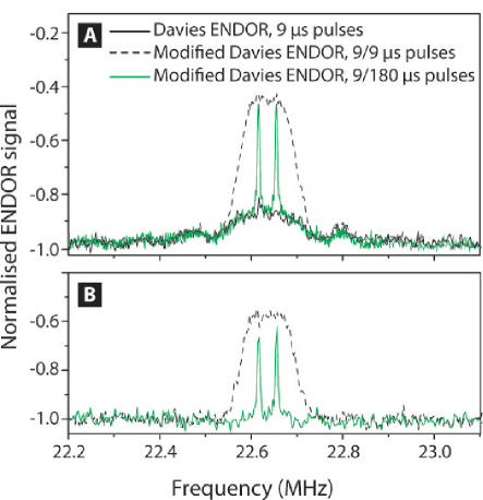
Figure 4: Spectral resolution enhancement in the modified Davies ENDOR experiment can be achieved by increasing the spectral selectivity of the second (recovery) RF pulse, as illustrated for the $M_{S}=-3/2$ ENDOR line of ¹⁴N@C₆₀, in CS₂ at 190 K. (A) A comparison of the traditional Davies ENDOR with a 9 $\mu$s RF pulse and the modified Davies ENDOR with an additional 9 $\mu$s recovery RF pulse demonstrates a significant enhancement in signal intensity. If the second RF pulse is lengthened (to 180 $\mu$s in this case), the selectivity of the recovery pulse increases and the enhanced component of the ENDOR line becomes better resolved. (B) The oscillating background is identical in all spectra in (A) and it can be removed from the modified Davies ENDOR spectra by subtracting the spectrum obtained with a traditional Davies ENDOR.

Figure 4 illustrates this effect for N@C₆₀, in which the intrinsic ¹⁴N ENDOR lines are known to be very narrow ($<1$ kHz). Increasing the duration of the recovery RF pulse from 9 $\rm{\mu}$s to 180 $\rm{\mu}$s dramatically increases the resolution and reveals two narrow lines, at no significant cost in signal intensity or experiment duration. In Figure 4B, what appears to be a single broad line is thus resolved into two, corresponding to two non-degenerate $\Delta M_{I}=1$ spin transitions of ¹⁴N $I=1$ nuclear spin at electron spin projection $M_{S}=-3/2$. We notice the presence of a broad oscillating background in the modified Davies ENDOR spectra in Figure 4A. This background matches the signal detected using a standard Davies ENDOR, where it is clearly seen to have a recognizable sinc-function shape (i.e. its modulus) and thus corresponds to the off-resonance excitation profile of the first RF pulse. As shown in Figure 4B, this background signal can be successfully eliminated from the modified Davies ENDOR spectra by subtracting the signal measured with a standard Davies ENDOR.

VI Measuring Nuclear Spin Relaxation Times T_1n

As already indicated in Figure 3A, the signal intensity in a traditional Davies ENDOR increases as the repetition time t_r is made longer, as compared to the nuclear spin relaxation time T_1n. It is shown in the Appendix that, in case when T${}_{1n}\sim$ t${}_{r}\gg$ T_1e, the ENDOR signal intensity varies as:

$$I_{\rm{ENDOR}}\sim 1-\exp{\left(-t_{r}/T_{1n}\right)}.$$ (2)

Thus, measuring the signal intensity in a traditional Davies ENDOR as a function of t_r yields a measure of T_1n, as illustrated in Figure 5A for ²⁸Si:P and in Figure 5B for N@C₆₀. In both cases, T_1n is found to be much longer than T_1e (cp. T${}_{1n}=280$ ms and T${}_{1e}=1$ ms for ²⁸Si:P at 10 K Tyryshkin et al. (2003), and T${}_{1n}=50$ ms and T${}_{1e}=0.32$ ms for ¹⁴N@C₆₀ in CS₂ at 190 K Morton et al. (2006)), as must be expected because nuclear spins have a smaller magnetic moment and are therefore less prone to fluctuating magnetic fields in the host environment.

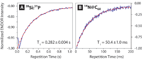
Figure 5: Intensity of the traditional Davies ENDOR signal as a function of repetition time measured for (A) ²⁸Si:P (52.33 MHz line) at 10 K, and (B) ¹⁴N@C₆₀ (22.626 MHz line) in CS₂ at 190 K. An exponential fit (dashed line) yields the respective nuclear spin relaxation time T_1n. In (A) the signal intensity at short times ($<0.1$ s) deviates from the exponential fit due to the transient effects arising from a finite electron spin T_1e time, as described in ref. Epel et al. (2001).

Using Davies ENDOR to measure nuclear spin relaxation times, T_1n and T_2n, has been already proposed, however the applicability of suggested pulse schemes has been limited to cases where T_1n (or T_2n) $<$ T_1e Höfer et al. (1986); Höfer (1994). Herein, we extend the method to (more common) cases where T_1n is greater than T_1e.

VII Conclusions

We have shown that signal intensity in the traditional Davies ENDOR experiment is strongly dependent on the experimental repetition time and that the addition of the second (recovery) RF pulse at the end of the pulse sequence eliminates this dependence. This modification to the Davies pulse sequence dramatically enhances the signal/noise (allowing signal acquisition at much faster rate without loss of the signal intensity), and can also improve the spectral resolution. We also demonstrate that the sensitivity of the Davies ENDOR to nuclear relaxation time can be exploited to measure T_1n. The technique of adding an RF recovery pulse after electron spin echo detection can be applied to the general family of pulsed ENDOR experiments, in which a non-thermal nuclear polarization is generated, including the popular technique of Mims ENDOR Schweiger and Jeschke (2001); Mims (1965).

Appendix

Here we describe how a compromise can be reached, using the traditional Davies ENDOR, between maximal ENDOR ‘per-shot’ signal and overall experiment duration. The equations below show the evolution of state populations — a quantitative equivalent of those shown in Figure 2 in the main text, with the difference that a partial nuclear relaxation is considered during the repetition time $t_{r}$. Thus, we assume T${}_{1n}\sim$ t${}_{r}\gg$ T_1e. Legend:

$$\left(\begin{array}[]{c}\uparrow_{e}\uparrow_{n}\\ \uparrow_{e}\downarrow_{n}\\ \downarrow_{e}\downarrow_{n}\\ \downarrow_{e}\uparrow_{n}\\ \end{array}\right),~{}~{}~{}~{}a=g\beta_{e}B/2kT~{}~{}~{}~{}~{}~{}~{}~{}~{}~{}~{}~{}~{}~{}~{}~{}~{}~{}~{}~{}~{}~{}~{}~{}~{}~{}~{}~{}~{}~{}~{}~{}~{}~{}~{}~{}~{}~{}~{}~{}~{}~{}~{}~{}~{}~{}~{}~{}~{}~{}~{}~{}~{}~{}~{}~{}~{}~{}~{}~{}~{}~{}~{}~{}~{}~{}~{}~{}~{}~{}~{}~{}~{}~{}~{}~{}~{}~{}~{}~{}~{}~{}~{}~{}~{}~{}~{}~{}~{}~{}~{}~{}~{}~{}~{}~{}~{}~{}~{}~{}~{}~{}~{}$$

1st shot:

$$\left(\begin{array}[]{c}-a\\ -a\\ +a\\ +a\\ \end{array}\right)\rightarrow\pi_{e}\rightarrow\left(\begin{array}[]{c}-a\\ +a\\ -a\\ +a\\ \end{array}\right)\rightarrow\pi_{n}\rightarrow\left(\begin{array}[]{c}+a\\ -a\\ -a\\ +a\\ \end{array}\right)\rightarrow e.s.e\rightarrow\left(\begin{array}[]{c}+a\\ -a\\ -a\\ +a\\ \end{array}\right)\rightarrow{\rm delay}~{}t_{r}\rightarrow\left(\begin{array}[]{c}-a(1-\exp{\left(-t_{r}/T_{1n}\right)})\\ -a(1+\exp{\left(-t_{r}/T_{1n}\right)})\\ +a(1-\exp{\left(-t_{r}/T_{1n}\right)})\\ +a(1+\exp{\left(-t_{r}/T_{1n}\right)})\\ \end{array}\right)$$

2nd and subsequent shots:

$$\left(\begin{array}[]{c}-a(1-\exp{\left(-t_{r}/T_{1n}\right)})\\ -a(1+\exp{\left(-t_{r}/T_{1n}\right)})\\ +a(1-\exp{\left(-t_{r}/T_{1n}\right)})\\ +a(1+\exp{\left(-t_{r}/T_{1n}\right)})\\ \end{array}\right)\rightarrow\pi_{e}\rightarrow\left(\begin{array}[]{c}-a(1-\exp{\left(-t_{r}/T_{1n}\right)})\\ +a(1-\exp{\left(-t_{r}/T_{1n}\right)})\\ -a(1+\exp{\left(-t_{r}/T_{1n}\right)})\\ +a(1+\exp{\left(-t_{r}/T_{1n}\right)})\\ \end{array}\right)\rightarrow\pi_{n}\rightarrow\left(\begin{array}[]{c}+a(1-\exp{\left(-t_{r}/T_{1n}\right)})\\ -a(1-\exp{\left(-t_{r}/T_{1n}\right)})\\ -a(1+\exp{\left(-t_{r}/T_{1n}\right)})\\ +a(1+\exp{\left(-t_{r}/T_{1n}\right)})\\ \end{array}\right)\rightarrow$$

$$\rightarrow e.s.e.\rightarrow\left(\begin{array}[]{c}+a(1-\exp{\left(-t_{r}/T_{1n}\right)})\\ -a\\ -a\\ +a(1+\exp{\left(-t_{r}/T_{1n}\right)})\\ \end{array}\right)\rightarrow{\rm delay}~{}t_{r}\rightarrow\left(\begin{array}[]{c}-a(1-\exp{\left(-t_{r}/T_{1n}\right)})\\ -a(1+\exp{\left(-t_{r}/T_{1n}\right)})\\ +a(1-\exp{\left(-t_{r}/T_{1n}\right)})\\ +a(1+\exp{\left(-t_{r}/T_{1n}\right)})\\ \end{array}\right)$$

The intensity of the ENDOR signal is therefore:

$$2a(1-\exp{\left(-t_{r}/T_{1n}\right)}).$$

As the signal-to-noise is proportional to the square root of the number of samples, and thus to $\sqrt{1/t_{r}}$, we can define a signal efficiency of:

$$2a(1-\exp{\left(-t_{r}/T_{1n}\right)})/\sqrt{t_{r}}.$$

This figure is maximized when $t_{r}\approx 1.25$ T_1n.

References

- Feher (1956) G. Feher, Phys. Rev. 103, 834 (1956).
- Kevan and Kispert (1976) L. Kevan and L. D. Kispert, Electron spin double resonance spectroscopy (Wiley, New York, 1976).
- Schweiger and Jeschke (2001) A. Schweiger and G. Jeschke, Principles of Pulse Electron Paramagnetic Resonance (Oxford University Press, Oxford, UK ; New York, 2001).
- Gemperle and Schweiger (1991) C. Gemperle and A. Schweiger, Chem. Rev. 91, 1481 (1991).
- Dalton and Kwiram (1972) L. R. Dalton and A. L. Kwiram, J. Chem. Phys. 57, 1132 (1972).
- Epel et al. (2001) B. Epel, A. Poppl, P. Manikandan, S. Vega, and D. Goldfarb, J. Magn. Reson. 148, 388 (2001).
- Davies (1974) E. R. Davies, Phys. Lett. A 47, 1 (1974).
- Mims (1965) W. B. Mims, Proc. Roy. Soc. London 283, 452 (1965).
- Itoh (2004) K. M. Itoh, private communication (2004).
- Kanai et al. (2004) M. Kanai, K. Porfyrakis, G. A. D. Briggs, and T. J. S. Dennis, Chem. Commun. 2, 210 (2004).
- Fletcher et al. (1954) R. C. Fletcher, W. A. Yager, G. L. Pearson, and F. R. Merritt, Phys. Rev. 95, 844 (1954).
- Feher (1959) G. Feher, Phys. Rev. 114, 1219 (1959).
- Murphy et al. (1996) T. A. Murphy, T. Pawlik, A. Weidinger, M. Hohne, R. Alcala, and J.-M. Spaeth, Phys. Rev. Lett. 77, 1075 (1996).
- Tyryshkin et al. (2003) A. M. Tyryshkin, S. A. Lyon, A. V. Astashkin, and A. M. Raitsimring, Phys. Rev.B 68, 193207 (2003).
- Morton et al. (2005) J. J. L. Morton, A. M. Tyryshkin, A. Ardavan, K. Porfyrakis, S. A. Lyon, and G. A. D. Briggs, J. Chem. Phys. 122, 174504 (2005).
- Epel et al. (2003) B. Epel, D. Arieli, D. Baute, and D. Goldfarb, J. Magn. Reson. 164, 78 (2003).
- Bowman and Tyryshkin (2000) M. K. Bowman and A. M. Tyryshkin, J. Magn. Reson. 144, 74 (2000).
- Morton et al. (2006) J. J. L. Morton, A. M. Tyryshkin, A. Ardavan, K. Porfyrakis, S. A. Lyon, and G. A. D. Briggs, J. Chem. Phys. 124, 014508 (2006).
- Höfer et al. (1986) P. Höfer, A. Grupp, and M. Mehring, Phys. Rev. A 33, 3519 (1986).
- Höfer (1994) P. Höfer, in 36th Rocky Mountain Conference on Analitycal Chemistry (Denver, CO, 1994), p. 103.