Dynamical Friction in Stellar Systems: an introduction

Abstract

An introductory exposition of Chandrasekhar’s gravitational dynamical friction, appropriate for an undergraduate class in mechanics, is presented. This friction results when a massive particle moving through a “sea” of much lighter star particles experiences a retarding force du to an exchange of energy and momentum. General features of dynamical friction are presented, both in an elementary and in a more elaborate way using hyperbolic two-body interactions. The orbital decay of a massive particle in an homogeneous gravitational system is solved analytically, that leads to an underdamped harmonic oscillator type of motion. A numerical integration of the equation of motion in a more realistic case is done. These results are compared to those of an $N$-body computer simulation. Several problems and projects are suggested to students for further study.

I Introduction

Classical mechanics, perhaps the oldest of the physical sciences, continues to be an area of intensive research, both in its foundationsMarsden and Ratiu (1999); Hestenes (1999) and applications,Murray and Dermot (1999); Diacu and Holmes (1996) and a source of discussion and examples in teaching. Applications range from the modeling of cellular mechanical processesBoal (2002) to solar system dynamicsMurray and Dermot (1999) and galactic systems.Binney and Tremaine (1987); Saslaw (2003); Aarseth (2003)

In describing nature students learn from their first courses, and particularly in laboratory experiments, that “the forces on a single thing already involve approximation, and if we have a system of discourse about the real world, then that system, at least for the present day, must involve approximations of some kind”; as mentioned by Feynman on introducing the subject of friction.Feynman et al. (1963)

This phenomenon is usually introduced in text-booksAlonso and Finn (1992); Halliday et al. (2002); Kittel et al. (1973); French (1971) and lectures by considering the slide of a material block on a surface, and a distinction between static and kinetic friction is made. A classical example of the effect of a friction-like force is the motion of a mass attached to a spring inside a viscous medium, where the corresponding differential equation is solved, and its behavior studied. At the end, one invariably needs to state that friction and its origin is a complicated matter, involving complex interactions at the atomic and molecular level among the surfaces in contact.Palmer (1949); Rabinowicz (1963); Krim (2002); Ringlein and Robbins (2004)

Several non-typical examples of mechanical friction for introductory courses exist,Parkyn (1958); Lapidus (1970); Molina (2004); Simbach and Priest (2005) that help both teachers and students alike in lectures on mechanics. All friction related problems are a background for discussing the important connection between the work-energy theorem and dissipative systems.Sherwood (1983); Mallinckrodt and Leff (1992); Arons (1999)

The purpose of this paper is to bring an example from astronomySagan (1980); Arny (1994); Shu (1982) closely related to standard mechanical friction, namely: dynamical friction. This process was first introduced in stellar systems by Subrahmanyan Chandrasekhar.Chandrasekhar (1943, 1960) In brief, a massive particle $m$ experiences a drag force when moving in a “sea” of much lighter star particles $m_{*}$ by exchanging energy and momentum. An elementary understanding requires only some basic ideas from mechanics, and hence suitable for presentation in introductory courses.

Dynamical friction is important in astronomical studies of, for example: the fate of galaxy satellitesWeinberg (1989); Velazquez and White (1999); Fujii et al. (2005) or globular clustersMcMillan and Portegies Zwart (2003) orbiting their host galaxies, the substructure of dark halos surrounding galaxies,van den Bosch et al. (1999); Zhao (2004); Bullock and Johnston (2005) and the motion of black holes in the centers of galaxies.Kim et al. (2004) It has been proposed to explain the formation of binaries in the Kuiper-beltGoldreich et al. (2002), and the migration of Jupiter-mass planets in other solar systems from the outer parts where they presumably formed ($\mathrel{\hbox to0.0pt{\lower 3.0pt\hbox{$\mathchar 536\relax$}\hss}\raise 2.0pt\hbox{$\mathchar 318\relax$}}1$ AU) to the small orbital distances ($\mathrel{\hbox to0.0pt{\lower 3.0pt\hbox{$\mathchar 536\relax$}\hss}\raise 2.0pt\hbox{$\mathchar 316\relax$}}0.1$ AU) at which they are observed.Del Popolo et al. (2003) It even has been considered in the motion of cosmic strings.Avelino and Shellard (1995)

The presentation of this topic to students, in a lower or upper-undergraduate class on mechanicsTaylor (2005); Kibble and Berkshire (2004) or computational physics,Spencer (2005) will enhance their appreciation of physics in describing nature and expose them to another example of classical mechanics. Furthermore, students will obtain a glimpse of an area of astronomical research important for the understanding of the fate and behavior of stellar systems.

The organization of this paper is as follows. In Section II basic elements of the theory of dynamical friction are presented. Firstly, elementary arguments are used to elucidate them. Secondly, Chandrasekhar’s approximation using two-body hyperbolic Keplerian collisions is considered. In Section III a simple analytical problem for the motion of a massive particle in an ideal homogeneous stellar system is solved; a damped harmonic oscillator is found. In Section IV a more realistic astronomical example that requires the numerical integration of the equation of motion is presented. Comparison with a computer experiment is done afterwards. Final comments as well as some ideas for problems and projects of further study are provided in Section IV. An appendix contains some astronomical units and standard units used in gravitational computer simulations.

II Dynamical Friction

Two equivalent approaches to compute the dynamical friction a massive particle $m$ experiences as it moves through a stellar system of much lighter stars $m_{*}$ are the following.Binney and Tremaine (1987) (1) Particle $m$ produces a region of star overdensity behind it, much like the wake behind the motion of a ship, that in turn exerts a gravitational pull on $m$ leading to its deceleration.Mulder (1983) (2) Particle $m$ moves in the “sea” of lighter particles $m_{*}$ and an energy exchange occurs, increasing that of the lighter ones at the expense of the heavy one leading to a breaking force for $m$. In the latter picture the basic features of dynamical friction are easier to compute and understand by elementary methods. Here the latter picture is taken.

II.1 Elementary estimate

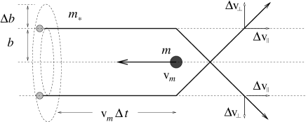
Figure 1: Illustration of the deceleration a heavy particle $m$ experiences when moving in an homogeneous and infinite “sea” of much lighter particles $m_{*}$.

Consider a particle $m$ moving with velocity $v_{m}$ in an homogeneous background of stationary lighter particles of equal mass $m_{*}$; see Figure 1. Assume only changes in kinetic energy. As $m$ moves through, a particle $m_{*}$ incoming with impact parameter $b$ will be given a velocity impulse of about the acceleration $a$ times the duration of the encounter $\Delta t$. This can be approximated as

$$\Delta v_{*}\approx\frac{Gm}{b^{2}}\times\frac{b}{v_{m}}\,.$$ (1)

The kinetic energy gain of $m_{*}$ is therefore

$$\Delta E_{*}\approx\frac{1}{2}m_{*}(\Delta v_{*})^{2}\approx\frac{1}{2}m_{*}\left(\frac{Gm}{bv}\right)^{2}\,.$$ (2)

The total change in velocity of the massive particle is given by accounting for all the encounters it suffers with particles $m_{*}$. The number of encounters with impact parameter between $b$ and $b+\Delta b$ is $\Delta N\approx n_{0}\,(v_{m}\Delta t)\,\Delta(\pi b^{2})$; where $n_{0}$ is the number density of background stars. The total change in velocity of $m$ at the expense of the energy lost by stars is then

$$\frac{{\rm d}v_{m}}{{\rm d}t}\approx\frac{1}{mv_{m}}\int\frac{{\rm d}E_{*}}{{\rm d}t}{{\rm d}N}\approx\frac{\pi G^{2}\rho_{0}m}{v_{m}^{2}}\int_{b_{\rm min}}^{b_{\rm max}}\frac{{\rm d}b}{b}\,,$$ (3)

where we set $\rho_{0}=n_{0}m_{*}$, the background density, and $b_{\rm min}$ and $b_{\rm max}$ are a minimum and maximum impact parameter, respectively. Letting $\ln\Lambda$ be the resulting integral, the deceleration of $m$ due to its interaction with an homogenous background of particles stars is

$$\frac{{\rm d}v_{m}}{{\rm d}t}\approx\frac{\pi G^{2}\rho_{0}m}{v_{m}^{2}}\ln\Lambda\,.$$ (4)

The velocity impulse on $m_{*}$ has a perpendicular $\Delta v_{\perp}$ and parallel $\Delta v_{||}$ component; see Figure 1. It is not difficult to see that a mean vector sum of all the $\Delta v_{\perp}$ contributions vanishes in this case. This is not true however for the mean square of $\Delta v_{\perp}$. Thus the dynamical friction force is along the line of motion of $m$.

Several key features of dynamical friction are observed from equation (4) in this elementary calculation, that appear also in more elaborate treatments. (1) The deceleration of the massive particle is proportional to its mass $m$, so the frictional force it experiences is directly proportional to $m^{2}$. (2) The deceleration is inversely proportional to the square of its velocity $v_{m}$.

II.2 Chandrasekhar formula

A further step in calculating the effect of dynamical friction is to consider hyperbolic Keplerian two-body encounters. Such analysis was done by Chandrasekhar.Chandrasekhar (1943, 1960) The resulting formula is provided in textbooks on stellar dynamics.Binney and Tremaine (1987) For completeness such calculations is provided here, following Binney & Tremaine.

Use of well known results from the Kepler problem for two bodies in hyperbolic encounters are used.Alonso and Finn (1992); Halliday et al. (2002); Kittel et al. (1973); French (1971); Coffman (1963) The two-body problem can be reduced to that of the motion of a particle of reduced mass $\mu=mm_{*}/(m+m_{*})$ about a fixed center of force:

$$\mu{\ddot{\mathbf{r}}}=-\frac{\kappa}{r^{2}}{\hat{\mathbf{r}}}\,,$$ (5)

where $\kappa=Gmm_{*}$, ${\mathbf{r}}={\mathbf{r}}_{*}-{\mathbf{r}}_{m}$ is the relative vector position of particles $m$ and $m_{*}$, and ${\hat{\mathbf{r}}}$ its unit vector; see Figure 2. The relative velocity is then ${\mathbf{V}}={\mathbf{v}}_{*}-{\mathbf{v}}_{m}$, and a change in it is

$$\Delta{\mathbf{V}}=\Delta{\mathbf{v}}_{*}-{\Delta\mathbf{v}}_{m}\,.$$ (6)

The velocity of the center-of-mass of $m$ and $m_{*}$ does not change, hence

$$m_{*}\,\Delta{\mathbf{v}}_{*}+m\,{\Delta\mathbf{v}}_{m}=0\,.$$ (7)

From equations (6) and (7) the change in velocity of $m$ is

$${\Delta\mathbf{v}}_{m}=-(\frac{m_{*}}{m+m_{*}})\,\Delta{\mathbf{V}}\,.$$ (8)

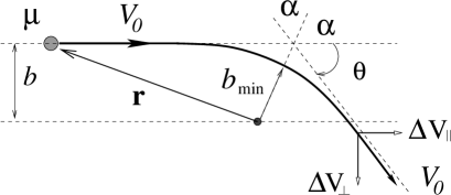
Figure 2: Dispersion of a “reduced” mass particle $\mu$ in the potential of a static body of mass $(m+m_{*})$ moving with relative speed $V_{0}$. The scattering angle is $\theta$.

Once $\Delta{\mathbf{V}}$ is determined, ${\Delta\mathbf{v}}_{m}$ can be found from equation (8). From the symmetry of the problem, is better to decompose $\Delta{\mathbf{V}}$ in terms of perpendicular and parallel components:

$$\Delta{\mathbf{V}}=\Delta{\mathbf{V}}_{||}+\Delta{\mathbf{V}}_{\perp}\,,$$ (9)

with

$$|\Delta{V}_{||}|=V_{0}\cos\theta\quad{\textrm{and}}\quad|\Delta{V}_{\perp}|=V_{0}\sin\theta\,,$$ (10)

where $\theta$ is the angle of dispersion and $V_{0}$ the initial speed at infinity; this being the same after the encounter since only kinetic energy changes are considered; see Figure 2. From geometry, the angle $\alpha$ in Figure 2 is related to the orbit’s eccentricity $e$ byAdolph et al. (1972)

$$\cos\alpha=\frac{1}{e}\quad\to\quad\cot\frac{\theta}{2}=\sqrt{e^{2}-1}\,,$$ (11)

where $\theta+2\alpha=\pi$. Physically $e$ is given by

$$e=\sqrt{1+\frac{2EL^{2}}{\mu^{3}\kappa^{2}}}\,,$$ (12)

where $E=\mu V_{0}^{2}/2$ in the kinetic energy and $L=\mu bV_{0}$ the angular momentum magnitude. Since

$$\sin\theta=\frac{2\tan\frac{\theta}{2}}{1+\tan^{2}\frac{\theta}{2}}\qquad{\textrm{and}}\quad\cos\theta=\frac{1-\tan^{2}\frac{\theta}{2}}{1+\tan^{2}\frac{\theta}{2}}\,,$$ (13)

after some algebra it is found that

$$|\Delta{V}_{\perp}|=\frac{2bV_{0}^{3}}{G(m+m_{*})}\left[1+\frac{b^{2}V_{0}^{4}}{G^{2}(m+m_{*})^{2}}\right]^{-1}\,,$$ (14)

$$|\Delta{V}_{||}|=2V_{0}\left[1+\frac{b^{2}V_{0}^{4}}{G^{2}(m+m_{*})^{2}}\right]^{-1}\,.$$ (15)

Using equation (8) the perpendicular and parallel magnitudes of the components of $\Delta{\mathbf{v}}_{m}$ follow:

$$|\Delta{\mathbf{v}}_{m\perp}|=\frac{2bmV_{0}^{3}}{G(m+m_{*})^{2}}\left[1+\frac{b^{2}V_{0}^{4}}{G^{2}(m+m_{*})^{2}}\right]^{-1}\,,$$ (16)

$$|\Delta{\mathbf{v}}_{m||}|=\frac{2mV_{0}}{(m+m_{*})}\left[1+\frac{b^{2}V_{0}^{4}}{G^{2}(m+m_{*})^{2}}\right]^{-1}\,.$$ (17)

In a homogeneous sea of stellar masses all perpendicular deflections cancel by symmetry. However, the parallel velocity changes are added and the mass $m$ will experience a deceleration.

The calculation of the total drag force due to a set of particles $m_{*}$ is as follows. Let $f(\mathbf{v}_{*})$ be the number density of stars. The rate at which particle $m$ encounters stars with impact parameter between $b$ and $b+{\rm d}b$, and velocities between ${\mathbf{v}}_{*}$ and ${\mathbf{v}}_{*}+{\rm d}{\mathbf{v}}_{*}$, is

$$2\pi b\,{\rm d}b\cdot V_{0}\cdot f(\mathbf{v}_{*})\,{\rm d}^{3}\mathbf{v}_{*}\,,$$ (18)

where ${\rm d}^{3}\mathbf{v}_{*}$ is the volume element in velocity space. The total change in velocity of $m$ is found by adding all the contributions of $|\Delta{\mathbf{v}}_{m||}|$ due to particles with impact parameters from $0$ to a $b_{\rm max}$ and then summing over all velocities of stars. At a particular $\mathbf{v}_{*}$ the change is

$$\frac{{\rm d}{\textbf{v}}_{m}}{{\rm d}t}\Big{|}_{{\mathbf{v}}_{*}}={\mathbf{V}}_{0}\cdot f(\mathbf{v}_{*})\,{\rm d}^{3}\mathbf{v}_{*}\int_{0}^{b_{\rm max}}|\Delta\mathbf{v}_{m||}|\,2\pi b\,{\rm d}b\,.$$ (19)

The required integral is

$${\cal I} = \int_{0}^{b_{\rm max}}\left[1+\frac{b^{2}V_{0}^{4}}{G^{2}(m+m_{*})^{2}}\right]^{-1}\,b\,{\rm d}b$$

$$=\int_{0}^{b_{\rm max}}\frac{b\,{\rm d}b}{1+ab^{2}}=\frac{1}{2a}\int_{1}^{s_{\rm max}}\frac{{\rm d}s}{s}\,,$$

where $a=V_{0}^{4}/G^{2}(m+m_{*})^{2}$ and $s=1+ab^{2}$, with $s_{\rm max}=1+ab^{2}_{\rm max}$. Evaluating the integral yields

$${\cal I}=\frac{1}{2}\frac{G^{2}(m+m_{*})^{2}}{V_{0}^{4}}\ln\left[1+\Lambda^{2}\right]\,,$$

where

$$\Lambda\equiv\frac{b_{\rm max}V_{0}^{2}}{G(m+m_{*})}=\frac{b_{\rm max}}{b_{\rm min}}\,.$$ (20)

Putting these results together in equation (19):

$$\frac{{\rm d}{\textbf{v}}_{m}}{{\rm d}t}\Big{|}_{{\mathbf{v}}_{*}} = 2\pi G^{2}\ln(1+\Lambda^{2})m_{*}(m+m_{*})$$ (21)

$$\times\;f(\mathbf{v}_{*})\,{\rm d}^{3}\mathbf{v}_{*}\frac{{\mathbf{v}}_{*}-{\mathbf{v}}_{m}}{|{\mathbf{v}}_{*}-{\mathbf{v}}_{m}|^{3}}\,.$$

The quantity $\ln\Lambda$ is called the Coulomb logarithm in analogy to an equivalent logarithm found in the theory of plasma. The factor $\ln\Lambda$ reflects the fact that the cumulative effect of small deflections is more important than strong or close encounters. This may be seen geometrically from Figure 2, were the stronger the deflection the smaller is the parallel component contributing to the slow down of $m$.

The determination of the limits $b_{\rm min}$ and $b_{\rm max}$ is not an easy matter and depends on the problem at hand. In this approximation $b_{\rm min}$ satisfies $V_{0}^{2}=Gm/b_{\rm min}$, where $V_{0}$ depends on the relative velocity of $m$ and $m_{*}$. If the motion of $m$ is relatively slow in comparison to that of the stars, $V_{0}$ can be approximated for example by the root-mean-square value velocity of stars $V_{\rm rms}$. The outer limit $b_{\rm max}$ is in principle the radius at which stars no longer can exchange momentum with $m$. If $m$ is close to the center of a stellar system $b_{\rm max}$ can be taken as a particular scale-radius of the system; for example, where the star density falls to half of its central value.

In typical astronomical applications $\Lambda\gg 1$. For example, consider the motion of a massive black hole of mass $m\approx 10^{5}{\rm M}_{\odot}$ near the center of a dwarf galaxy. These galaxies have $V_{\rm rms}\approx V_{0}\approx 30~{}$km s^-1, characteristic radii $b_{\rm max}\approx 3~{}$kpc and stars of masses $m_{*}\approx 1{\rm M}_{\odot}$. Using these values we obtain $\Lambda\approx 6.3\times 10^{3}$. This allows to use the approximation $\ln(1+\Lambda^{2})\approx 2\ln\Lambda$. Note that $\ln\Lambda$ shows a weak dependence on $V_{0}$ that is usually neglected. Values of $2\mathrel{\hbox to0.0pt{\lower 3.0pt\hbox{$\mathchar 536\relax$}\hss}\raise 2.0pt\hbox{$\mathchar 316\relax$}}\ln\Lambda\mathrel{\hbox to0.0pt{\lower 3.0pt\hbox{$\mathchar 536\relax$}\hss}\raise 2.0pt\hbox{$\mathchar 316\relax$}}20$ are typically found in astronomical literature.

Now, the integration of equation (21) over the velocity space of stars is required. Writing equation (21) as

$$\frac{{\rm d}{\textbf{v}}_{m}}{{\rm d}t} = G\int_{0}^{\infty}\frac{\rho({\mathbf{v}}_{*})({\mathbf{v}}_{*}-{\mathbf{v}}_{m})}{|{\mathbf{v}}_{*}-{\mathbf{v}}_{m}|^{3}}\,{\rm d}^{3}{\mathbf{v}}_{*}\,,$$ (22)

$$\rho({\mathbf{v}}_{*}) \equiv \vphantom{\int}4\pi G(m+m_{*})m_{*}\ln\Lambda f(\mathbf{v}_{*})\,,$$

it is noticed that represents the equivalent problem of finding the gravitational field (acceleration) at the “spatial” point ${\mathbf{v}}_{m}$ generated by the “mass density” $\rho({\mathbf{v}}_{*})$. From gravitational potential theory,Binney and Tremaine (1987); Collins II (1989) the acceleration at a particular spatial point ${\mathbf{r}}$ is given by

$${\textbf{a}}({\bf r})=G\int_{0}^{\infty}\frac{\rho({\mathbf{r}}^{\prime})({\mathbf{r}}^{\prime}-{\mathbf{r}})\,{\rm d}^{3}{\mathbf{r}}^{\prime}}{|{\mathbf{r}}^{\prime}-{\mathbf{r}}|^{3}}=-\frac{G{\mathbf{r}}}{r^{3}}\int_{0}^{r}\rho({\mathbf{r}}^{\prime})\,{\rm d}^{3}{\mathbf{r}}^{\prime}\,.$$

This is the known result that only matter inside a particular radius contributes to the force. In analogy to the gravitational case, the acceleration is given by the total “mass” inside $v_{*}<v_{m}$, is

$$\frac{{\rm d}{\textbf{v}}_{m}}{{\rm d}t}=-\frac{G{\mathbf{v}_{m}}}{v_{m}^{3}}\int_{0}^{v_{m}}\rho({\mathbf{v}}_{*})\,{\rm d}^{3}{\mathbf{v}}_{*}\,.$$

For an isotropic velocity distribution:

$$\frac{{\rm d}{\textbf{v}}_{m}}{{\rm d}t} = -{\cal C}_{\rm df}\,\mathbf{v}_{m}\,,$$ (23)

$${\cal C}_{\rm df} \equiv 16\pi^{2}G^{2}m_{*}(m+m_{*})\ln\Lambda\int_{0}^{v_{m}}f(v_{*})v_{*}^{2}\,{\rm d}v_{*}\,.$$

This is called Chandrasekhar dynamical friction formula. It shows that only stars moving slower than $v_{m}$ contribute to the drag force on the massive particle.

If stars have a Maxwellian velocity distribution function,

$$f(v_{*})=\frac{n_{0}}{(2\pi\sigma^{2})^{3/2}}\,{\rm e}^{-v_{*}^{2}/(2\sigma^{2})}\,,$$ (24)

the integral in (23) in done by an elementary method. In dimensionless form it is

$${\cal I}_{m}=\frac{n_{0}}{\pi^{3/2}}\int_{0}^{X}{\rm e}^{-y^{2}}y^{2}\,{\rm d}y\,,$$

where $y^{2}=v_{*}^{2}/2\sigma^{2}$ and $X\equiv v_{m}/(\sqrt{2}\sigma)$. Integrating by parts results in

$${\cal I}_{m}=\frac{n_{0}}{4\pi}\left[{\rm Erf}(X)-\frac{2X}{\sqrt{\pi}}\,{\rm e}^{-X^{2}}\right]\,,$$

where ${\rm Erf}(x)=(2/\sqrt{\pi})\int_{0}^{x}{\rm e}^{-y^{2}}{\rm d}y$ is the error function. If $\rho_{0}=n_{0}m_{*}$, the density of the background of stars, and assume that $m\gg m_{*}$, the deceleration of $m$ inside an homogeneous stellar system with isotropic velocity distribution is:

$$\frac{{\rm d}{\textbf{v}}_{m}}{{\rm d}t} = -\Gamma_{\rm df}\,\mathbf{v}$$ (25)

$$\Gamma_{\rm df} \equiv -\frac{4\pi G^{2}\ln\Lambda\rho_{0}m}{v_{m}^{3}}\left[{\rm Erf}(X)-\frac{2X}{\sqrt{\pi}}\,{\rm e}^{-X^{2}}\right].$$

III An Analytical Example

A simple application of Chandrasekhar’s formula (25) for an homogeneous spherically symmetric stellar system, although not infinite, is presented. The problem consists in determining the motion of a massive particle $m$ subject to gravitational and dynamical friction forces. The stellar system has a radius $R$ and total mass $M$; see Figure 3. The equation of motion for $m$ is

$$m\frac{{\rm d}^{2}{\mathbf{r}}}{{\rm d}t^{2}}={\mathbf{F}}_{\rm g}+{\mathbf{F}}_{\rm df}=-m\nabla\varphi(r)+m\,{\mathbf{a}}_{\rm df}\,,$$ (26)

where $\varphi(r)$ is the gravitational potential, and $\mathbf{a}_{\rm df}$ is given by equation (25).

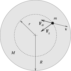
Figure 3: Forces acting on a massive particle $m$ moving with velocity $\mathbf{v}$ inside a stellar system: $\mathbf{F}_{\rm g}$ is the gravitational force and $\mathbf{F}_{\rm df}$ the dynamical friction force. The latter acting opposite to the direction of motion of $m$.

Equation (26) is not in general tractable by analytical methods, so some approximations are required. ZhaoZhao (2004) has found an approximation to the term associated with the velocity distribution in equation (25), namely:

$$\chi(X)\equiv\frac{1}{X^{3}}\left[{\rm{Erf}}(X)-\frac{2X}{\sqrt{\pi}}{\rm e}^{-X^{2}}\right]\approx\frac{1}{\frac{4}{3}+X^{3}}\,,$$ (27)

that works to within 10 percent for $0\leq X<\infty$. When $m$ moves slow in comparison to the velocity dispersion of stars, $v\ll\sigma$, $\chi(0)\approx 3/4$, and when $v=\sigma/2\,$ $\chi(1)\approx 3/7$. Note that in the case of a very fast relative motion of $m$ dynamical friction is negligible; a situation analogous to when a block of material slides fast. Using the previous approximation, and considering $\chi=3/4$, the frictional force $\mathbf{F}_{\rm df}$ in equation (26) becomes:

$${\mathbf{F}}_{\rm df}=m{\mathbf{a}}_{\rm df}\approx-\frac{3\pi G^{2}\ln\Lambda\rho_{0}m^{2}}{(\sqrt{2}\sigma)^{3}}\,\mathbf{v}=-\gamma\,\mathbf{v}\,,$$ (28)

where $\gamma=3\pi G^{2}\ln\Lambda\rho_{0}m^{2}/(\sqrt{2}\sigma)^{3}$.

To determine $\mathbf{F}_{\rm g}$ recall that the potential is related to the density through Poisson equation,

$$\nabla^{2}\varphi(r)=4\pi G\rho(r)\,,$$ (29)

whose solution for a spherically symmetrical system of radius $R$ is

$$\varphi(r)=-4\pi G\left[\frac{1}{r}\int_{0}^{r}\rho(r)r^{2}\,{\rm d}r+\int_{r}^{R}\rho(r)r\,{\rm d}r\right]\,.$$ (30)

In a constant density $\rho_{0}$ system the potential is

$$\varphi(r)=-2\pi G\rho_{0}\,(R^{2}-\frac{1}{3}r^{2})\,,$$ (31)

and the gravitational force on $m$ is

$${\mathbf{F}}_{\rm g}=-m\nabla\varphi(r)=-\frac{4}{3}\pi G\rho_{0}m\,{\mathbf{r}}=-k\,{\mathbf{r}}\,,$$ (32)

with $k=4\pi G\rho_{0}m/3$. This is the well known result from introductory mechanics that a particle inside an homogeneous gravitational system performs a harmonic motion.

Combining equations (28) and (32) the resulting equation of motion is

$$m\frac{{\rm d}^{2}{\mathbf{r}}}{{\rm d}t^{2}}+k\,{\mathbf{r}}+\gamma\,\mathbf{v}=0\,.$$ (33)

This is the same equation, for example, as that of a mass attached to a spring with stiffness constant $k$ inside a medium of viscosity $\gamma$; i.e., a damped harmonic oscillator.Alonso and Finn (1992); Halliday et al. (2002); Kittel et al. (1973); French (1971) The solution of equation (33) in a plane, under arbitrary initial conditions

$$x(0)=x_{0},\quad{\dot{x}}(0)=u_{0}\,;\quad\quad y(0)=y_{0},\quad{\dot{y}}(0)=v_{0}\,,$$

where the dot indicates a time derivative, isWeinstock (1961); Luthar (1979)

$$x(t) = \frac{{\rm e}^{-(\beta+\xi)t}}{2R}\left\{({\rm e}^{2\xi t}-1)u_{0}+\right.$$

$$\left.\left[({\rm e}^{2\xi t}-1)\beta+({\rm e}^{2\xi t}+1)\xi\right]x_{0}\right\}\,,$$

$$y(t) = \frac{{\rm e}^{-(\beta+\xi)t}}{2\xi}\left\{({\rm e}^{2\xi t}-1)v_{0}+\right.$$ (34)

$$\left.\left[({\rm e}^{2\xi t}-1)\beta+({\rm e}^{2\xi t}+1)\xi\right]y_{0}\right\}\,,$$

where $2\beta=\gamma/m$ and $\xi=\sqrt{\beta^{2}-\omega_{0}^{2}}$, with $\omega_{0}^{2}=k/m$.

The behavior of $m$ is dictated by the relative values of $\beta$ and $\omega$. The values of $\ln\Lambda$ and $\sigma$ are first to be estimated. Take $b_{\rm max}\approx R$ and $b_{\rm min}=Gm/V_{0}^{2}$. An estimate of $V_{0}$ may be obtained from the virial theorem,Alonso and Finn (1992) that relates the kinetic $T$ and potential energy $W$ of the system by:

$$2T=-W\,.$$ (35)

For an homogeneous system of size $R$ the potential energy is

$$W=-4\pi G\int_{0}^{R}\rho_{0}Mr\,{\rm d}r=-\frac{3}{5}\frac{GM^{2}}{R}\,,$$ (36)

and the kinetic energy is taken as $T=MV_{0}^{2}/2$. This leads to

$$V_{0}^{2}\approx\frac{3}{5}\frac{GM}{R}\approx 3\sigma^{2}\,;$$ (37)

where the last term provides an estimate of the one-dimensional velocity dispersion under the assumption of isotropy in the velocity distribution of stars. Using equation (37) $\beta$ and $\omega$ are:

$$\beta=\frac{45}{16}\sqrt{\frac{5}{2}}\frac{G^{2}mM\ln\Lambda}{R^{3}(GM/R)^{3/2}}\,,\quad\quad\omega_{0}=\sqrt{\frac{GM}{R^{2}}}\,.$$ (38)

The resulting Coulomb logarithm is $\ln\Lambda=\ln[3M/(5m)]$.

To compare the numerical values of $\beta$ and $\omega_{0}$ is better to use another system of units than a physical one. Let $G\!=\!M\!=\!R\!=\!1$, that is a common choice in $N$-body simulations in astronomy; to return to physical units one can use Newton’s law and set $G$ to the appropriate value (see Appendix). In these units, relations (38) become

$$\beta=\frac{45}{16}\sqrt{\frac{5}{2}}m\ln\left(\frac{3}{5m}\right)\,,\quad\quad\omega_{0}=1\,.$$ (39)

If $m=1/100$ then $\ln\Lambda\approx 4$ and $\beta\approx 0.2<\omega_{0}$. Hence an underdamped harmonic motion for the massive particle results. If $m=1/10$ then $\ln\Lambda\approx 2$ and $\beta\approx 0.8\approx\omega_{0}$, so the motion of $m$ will be strongly damped. Note that an upper limit to $m$ is set when $m=3/5$, leading to $\ln\Lambda=0$; i.e., no dynamical friction results. For larger $m$ a negative $\beta$ is obtained. Clearly, the model fails and the behavior of the dynamics is unrealistic.

For cases of interest, where $m\ll M$, it follows that $\beta<\omega_{0}$ and the resulting motion (34), after some algebra, is

$$x(t) = \left[x_{0}\cos\omega t+\frac{u_{0}+\beta x_{0}}{\omega}\sin\omega t\right]{\rm e}^{-\beta t}\,,\quad$$

$$y(t) = \left[y_{0}\cos\omega t+\frac{v_{0}+\beta y_{0}}{\omega}\sin\omega t\right]{\rm e}^{-\beta t}\,,$$ (40)

where $\omega^{2}=\omega_{0}^{2}-\beta^{2}$. Note that a time-scale when the orbit decays $1/{\rm e}$ is given by $\tau_{\rm df}=1/\beta$.

Take as example $m=0.01$. If the initial position of $m$ is at $(x,y)=(0.59,0.0)$ and its velocity $(0.0,0.44)$ the resulting orbit is that shown in Figure 4-left with solid line. Doubling $m$ results in the orbit shown in Figure 4-right. The dashed lines in correspond to the orbit of $m$ without dynamical friction. The effect of increasing the mass of $m$ on the orbit, and on the decay time $\tau_{\rm df}$, is clearly appreciated.

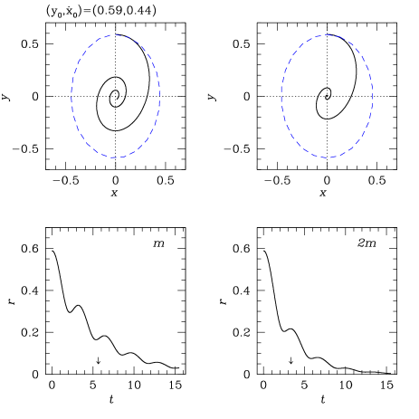
Figure 4: Orbital decay of a massive particle $m$ in a homogeneous stellar system due to dynamical friction. Initial conditions are $(x_{0},y_{0})=(0,0.59)$ and $(u_{0},v_{0})=(0.44,0)$. Left panels are for $m=0.01$ and right ones for $m=0.02$. Top panels show the orbit (solid line) in the xy-plane and bottom ones the time evolution of the distance $r$ from the center. The dynamical friction time scale $\tau_{\rm df}=1/\beta$ is indicated by an arrow. Dashed lines are orbits without considering dynamical friction.

This example shows the basic features of, for example, the orbital decay of a satellite galaxy toward the center of its host larger galaxy. It may be applied also to the motion of a massive black hole near the center of a galaxy or star cluster, where to some approximation the gravitational potential can be taken as harmonic. More realistic situations require however the numerical integration of the orbit and/or an $N$-body computer simulation. A particular case of these are treated next.

IV A more realistic example

Chandrasekhar’s formula (25) although derived assuming an infinite homogeneous system may be applied, to some degree, when stellar systems are non-homogeneous.Binney and Tremaine (1987) In this case, local values for the density $\rho(r)$ and the velocity dispersion $\sigma(r)$ are used. Here the motion of a massive particle $m$ inside a non-homogeneous stellar system is considered, both using a semi-analytical method and $N$-body simulation, to illustrate further the application of dynamical friction.

IV.1 Semi-analytic treatment

A simple representation of a stellar system, such as a globular cluster or an elliptical galaxy, is provided by the Plummer model. Its potential and stellar density are, respectively:Binney and Tremaine (1987); Saslaw (2003)

$$\varphi(r)=-\frac{GM}{(r^{2}+a^{2})^{1/2}},\quad\rho(r)=\frac{3Ma^{2}/4\pi}{(r^{2}+a^{2})^{5/2}},$$ (41)

where $M$ is the total mass, and $a$ the scale-radius of the system. In a spherical system with isotropic velocity distribution the equation of “hydrostatic” equilibrium is satisfied:

$$\frac{1}{\rho}\frac{{\rm d}(\rho\sigma^{2})}{{\rm d}r}=-\frac{{\rm d}\varphi}{{\rm d}r}\quad\rightarrow\quad\sigma^{2}(r)=-\frac{\varphi(r)}{6}\,.$$ (42)

The last result follows from noticing that $\rho\propto\varphi^{5}$, and imposing boundary conditions that both $\rho\sigma^{2}$ and $\varphi$ go to zero at infinity.

Equations (41) and (42) will be used in equation (25) to compute the orbital motion of a massive particle $m$. It rests to determine $b_{\rm min}$ and $b_{\rm max}$. The former is evaluated at local values, $b_{\rm min}\!=\!Gm/[3\sigma^{2}(r)]$, and the latter is set fix to $b_{\rm max}\!=\!a$.

The equation of motion (26) for $m$ can now be integrated numerically using standard methods,Press et al. (1992); Garcia (2000) or using the one discussed by FeynmanFeynman et al. (1963) for planetary orbits ($\S$9). Here a fourth-order Runge-Kutta algorithm with adaptive time-step was used. The initial conditions for $m$ are the same as those used in the analytical case.

In Figure 5 the resulting orbit from the numerical integration is shown as a dashed line. Also, the behavior of the $x$ and $y$ coordinates, and of the distance $r$ of $m$ to the center, as a function of time are shown. The typical decay of the orbit is evident. In the same figure results from an $N$-body simulation are displayed, that are described next.

IV.2 N-body simulation

The use of $N$-body simulations allows to study more realistically the different dynamical phenomena that occur in stellar systems.Hockney and Eastwood (1988); Aarseth (2003) Several $N$-body codes with different degrees of sophistication have been developed for astronomical problems in mind.Barnes and Hut (1986); Springel (2005); Dehnen (2000) Some low-$N$ simulations can be run nowadays using a personal computer with publicly available $N$-body codes.

Barnes’ tree-code in Fortran, and some of his public subroutines are used to simulate the motion of $m$ inside a Plummer model. A numerical realization of this model with $N=10^{5}$ particles is used with individual “star” masses of $m_{*}=1/N$. The massive particle $m=1/100$ with initial conditions $(y_{0},{\dot{x}}_{0})=(0.59,0.44)$ is set “by hand” inside the numerical Plummer model. In $N$-body units the scale radius is $a=3\pi/16=0.59$ (see Appendix).

The circular period at radius $r$ is $\tau=2\pi r/V_{\rm c}(r)$, where the circular velocity and integrated mass for a Plummer model are given, respectively, by:

$$V_{\rm c}(r)=\sqrt{\frac{GM(r)}{r}}\,,\quad\quad M(r)=\frac{M\,(r/a)}{[1+(r/a)^{2}]^{3/2}}\,.$$

From this, an orbital period of $\tau_{\rm a}=4.8$ time units at $r=a$ results. The simulation was run for $t=10\approx 2\tau_{\rm a}$ time units. The parameters for running the tree-code in serial were those provided by Barnes at his Internet site for an isolated Plummer evolution. The quadrupole moment in the gravitational potential is activated. The simulation took about 5.2 cpu hours on a PC with an Athlon 2.2GHz processor, and 512 KB of cache size. Energy conservation was $\leq 0.04$ percent, that is considered very good.

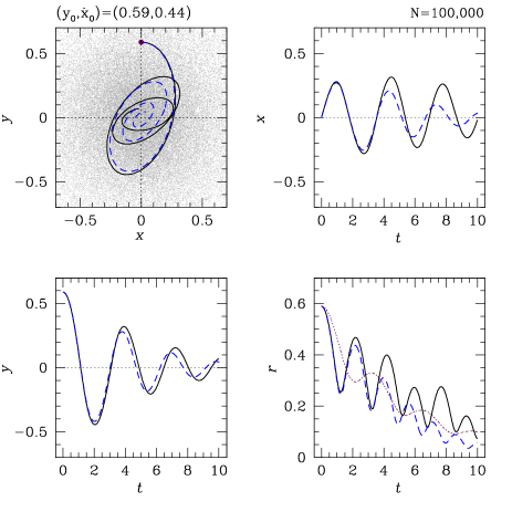
Figure 5: $N$-body simulation of the orbital decay (solid line) of a massive particle $m$ inside a Plummer stellar model. The semi-analytical (dashed line) and the analytical calculation (dotted line) of Figure 4 are drawn for comparison. These overestimate the effect of dynamical friction in comparison to the numerical simulation.

Figure 5 shows the orbital evolution of the massive particle $m$ in the $N$-body system as a solid line. The dashed line corresponds to the semi-analytical calculation of Section IV.1. This follows closely the orbit of $m$ in the $N$-body simulation for about $\tau_{\rm a}$ time units. Afterwards, it deviates from the $N$-body result. In the $r$-$t$ panel, the analytical solution (40) is shown as a dotted line; that is, assuming the total system was homogeneous.

Both approximations overestimate the decay rate of $m$ in comparison to the $N$-body simulation. Taking $b_{\rm max}=a/5$ leads to a somewhat better agreement, but does not reproduce the $N$-body result. Rather surprisingly, the analytical result does a fair job in reproducing the overall orbital decay in this case.

V Final Comments

The approximations in deriving Chandrasekhar formula limits, obviously, its application to more complex stellar systems than the one considered here. However, it is remarkable that equation (21) leads to reasonably well results when used with values under a local approximation.

In similar vain to the study of the friction between surfaces,Rabinowicz (1963); Krim (2002); Ringlein and Robbins (2004) dynamical friction is a complex subject. Elaborate calculations based on Brownian motion,Chandrasekhar (1949) linear response theory, resonances, and the fluctuation-dissipation theorem exist.Bekenstein and Maoz (1992); Weinberg (1989); Nelson and Tremaine (1999) These that are steps forward toward a more complete physical theory for this process.

Instead of listing explicitly some of the shortcomings of Chandrasekhar dynamical friction formulaBinney and Tremaine (1987) when applied to gravitational systems, the student is encourage to think on some of them and possible improvements on such formula.

From the point of view of an introductory or intermediate class on mechanics the exposure of students to non-typical problems, as the one presented here contributes to further their understanding and appreciation of the subject.

Some ideas that may lead to problems and/or projects for students are:

1. How would the analytical solution considered here would be changed if the Plummer model is used? What type of approximations would be required to make? How does $\ln\Lambda$ change?

2. If $\sigma^{2}$ is a measure of the kinetic energy per unit mass of stars, what is an estimate for its mean increase due to the energy lost by the massive particle during its decay?

3. How would the orbital decay time be changed for different types of initial eccentricities of the massive particle?

4. Consider a star cluster ($m=10^{6}\,{\rm M}_{\odot}$) in circular orbit at a distance of $r=5\,{\rm kpc}$ from the center of our galaxy ($M\approx 6\times 10^{11}{\rm M}_{\odot}$, $R\approx 150\,$kpc). Would it be expected to fall to the center within the age of the universe, say $t=10^{10}\,$yr? Typical velocities for stars and dark matter particles at that distance are about $200$ km/s, and the scale-radius may be around 5 kpc. What if instead of a star cluster we have a galaxy satellite, such as the Magellanic Clouds, with $m\approx 10^{10}\,{\rm M}_{\odot}$ and at a distance of $100\,$kpc?

5. How do results change if instead of a Plummer model a more pronounced density profile is used, such as the HernquistHernquist (1990) model? How does the number of particles $N$ in a simulation affect the decay rate?

6. As the massive particle moves through the stellar system it induces a density wake behind it. Can this be detected in an $N$-body simulation on a home computer? How about looking for this wake in the phase-space diagram (e.g. a plot of ${\dot{x}}$–$x$) of stars near the the massive particle?

7. How good do the local approximation works if instead of a massive particle one has an extended object, small in comparison to its host galaxy?

Textbook problems are designed in general to yield one correct answer, the above ideas for problems are rather vague but this is on purpose. The reason is twofold. On one hand, to promote in students a spirit of research by setting an approximate physical model and to look for the required data and “tools” to solve it; some of them can be found in the references. On the other hand, no single definite answer can be given. A feature proper of the way physics evolves toward describing and understanding nature.

Appendix A Astronomical and N-body Units

Several quantities in astronomy are so large in comparison to common “terrestial” values, that special units are used. Table 1 lists some of these and their equivalences in physical units.

Table 1: Astronomical units

Unit	Equivalence
Astronomical unit	${\rm{AU}}=1.496\times 10^{11}\,$m
Parsec	pc=$\,2.063\times 10^{5}\,$AU
	pc=$\,3.261$ light-years
Kiloparsec	kpc=$10^{3}\,$ pc
Solar mass	M${}_{\odot}=1.989\times 10^{30}\,$kg
Year	yr = $3.156\times 10^{7}\,$s

In the mks system of units the Gravitational constant is $G=6.67\times 10^{-11}\,$m³ kg^-1 s^-2. A natural system of units for gravitational interactions is that where the gravitational constant is set to $G=1$; in the same way as for quantum systems Planck’s constant is usually set to $\hbar=1$. On dimensional grounds $[G]=u_{v}^{2}u_{l}/u_{m}$; where $u_{m}$, $u_{l}$, and $u_{v}$ correspond, respectively, to units of mass, length and velocity.

The Gravitational constant can be expressed in terms of typical astronomical values, for example, as:

$$G=4.3007\times 10^{-3}\frac{{\rm km}^{2}{\rm pc}}{{\rm s}^{2}\,{\rm M}_{\odot}}=4.4984\times 10^{-3}\frac{{\rm pc}^{3}}{{\rm Myr}\,{\rm M}_{\odot}}\,.$$

The transformation of $G$ using length units such as kpc or Mpc ($10^{6}\,$pc) is direct. Choosing $u_{l}$ and $u_{m}$ the unit of velocity and of time $u_{t}$, under an appropriate $G$ value, are

$$u_{v}=\sqrt{\frac{Gu_{m}}{u_{l}}}\,,\qquad u_{t}=\sqrt{\frac{u_{l}^{3}}{Gu_{m}}}\,.$$

In this way the transformation from $N$-body units, where $G=M=R=1$, to physical ones can be made. Table 2 lists some values for different choices of $u_{l}$ and $u_{m}$, and the resulting units of $u_{v}$ and $u_{t}$. The entries correspond to using the approximate size and mass of a globular cluster, a disk of a spiral galaxy, and of a cluster of galaxies, respectively, as units $u_{l}$ and $u_{m}$.

Table 2: From $N$-body units to astronomical

Stellar system	$u_{l}$	$u_{m}$	$u_{v}$	$u_{t}$
		M⊙	km/s	Myr
Globular cluster	50 pc	$10^{6\hphantom{1}}$	9.3	5.3
Galaxy	10 kpc	$10^{11}$	207.4	47.2
Cluster of galaxies	$\;\;5$ Mpc	$10^{15}$	927.4	5271.4

In the standardized gravitational $N$-body unitsHeggie and Mathieu (1985); Aarseth (2003) the total energy of a system is $E=-1/4$. This follows from the virial theorem ($2T+W=0$), where

$$W=-\frac{1}{2}\frac{GM}{R}\quad\to\quad E=\frac{W}{2}=\frac{GM}{4R}.$$

Here $R$ is strictly what is called the virial radius of the system; that does not necessarily coincides with the total extent of the stellar system, but is a very good approximation. The potential energy of a Plummer model is

$$W=\frac{1}{2}\int_{0}^{\infty}\rho(r)\varphi(r)4\pi r^{2}\,{\rm d}r=-\frac{3\pi}{32}\frac{GM^{2}}{a}\,.$$

Thus the total energy is $E=-(3\pi GM^{2})/(64a)$. In $N$-body units this leads to a value of the Plummer scale-radius of $a=3\pi/16$.

References

- Marsden and Ratiu (1999) J. E. Marsden and T. S. Ratiu, Introduction to Mechanics and Symmetry (Springer, NY, 1999).
- Hestenes (1999) D. Hestenes, New Foundations for Classical Mechanics (Kluwer, Dordrecht, 1999).
- Murray and Dermot (1999) C. D. Murray and S. F. Dermot, Solar System Dynamics (Cambridge University Press, NY, 1999).
- Diacu and Holmes (1996) F. Diacu and P. Holmes, Celestial encounters: the origins of chaos and stability (Princeton University Press, NJ, 1996).
- Boal (2002) D. Boal, Mechanics of the Cell (Cambridge University Press, Cambridge, 2002).
- Binney and Tremaine (1987) J. Binney and S. Tremaine, Galactic Dynamics (Princeton University Press, NJ, 1987).
- Saslaw (2003) W. C. Saslaw, Gravitational Physics of Stellar and Galactic Systems (Cambridge University Press, Cambridge, 2003).
- Aarseth (2003) S. J. Aarseth, Gravitational -body Simulations (Cambridge University Press, Cambridge, 2003).
- Feynman et al. (1963) R. P. Feynman, R. B. Leighton, and M. Sands, Feynman lectures on physics, Volume 1 (Addison-Wesley, MA, 1963).
- Alonso and Finn (1992) M. Alonso and E. Finn, Physics (Addison-Wesley, MA, 1992).
- Halliday et al. (2002) D. Halliday, R. Resnick, and K. S. Krane, Physics, Volume 1 (Wiley, NY, 2002).
- Kittel et al. (1973) C. Kittel, W. Knight, and M. A. Ruderman, Mechanics. Berkeley Physics Course, Volume 1 (McGraw-Hill, NY, 1973).
- French (1971) A. P. French, Newtonian Mechanics. MIT Introductory Physics Series, Volume 1 (Norton, NY, 1971).
- Palmer (1949) F. Palmer, Am. J. Phys. 17, 336 (1949).
- Rabinowicz (1963) E. Rabinowicz, Am. J. Phys. 31, 897 (1963).
- Krim (2002) J. Krim, Am. J. Phys. 70, 890 (2002).
- Ringlein and Robbins (2004) J. Ringlein and M. O. Robbins, Am. J. Phys. 72, 884 (2004).
- Parkyn (1958) D. G. Parkyn, Am. J. Phys. 26, 436 (1958).
- Lapidus (1970) I. R. Lapidus, Am. J. Phys. 38, 1360 (1970).
- Molina (2004) M. I. Molina, Phys. Teach. 42, 485 (2004).
- Simbach and Priest (2005) J. C. Simbach and J. Priest, Am. J. Phys. 73, 1079 (2005).
- Sherwood (1983) B. Sherwood, Am. J. Phys. 51, 597 (1983).
- Mallinckrodt and Leff (1992) A. J. Mallinckrodt and H. S. Leff, Am. J. Phys. 60, 356 (1992).
- Arons (1999) A. B. Arons, Am. J. Phys. 67, 1063 (1999).
- Sagan (1980) C. Sagan, Cosmos (Random House, NY, 1980).
- Arny (1994) T. T. Arny, Explorations: an introduction to astronomy (Mosby-Year Book, MO, 1994).
- Shu (1982) F. H. Shu, Physical Universe (University Science Books, CA, 1982).
- Chandrasekhar (1943) S. Chandrasekhar, Astrophys. J. 97, 255 (1943).
- Chandrasekhar (1960) S. Chandrasekhar, Principles of Stellar Dynamics (Dover, NY, 1960).
- Weinberg (1989) M. D. Weinberg, Mon. Not. R. Astron. Soc. 239, 549 (1989).
- Velazquez and White (1999) H. Velazquez and S. D. M. White, Mon. Not. R. Astron. Soc. 304, 254 (1999).
- Fujii et al. (2005) M. Fujii, Y. Funato, and J. Makino, Publ. Astron. Soc. Jap. (2005), eprint astro-ph/0511651.
- McMillan and Portegies Zwart (2003) S. L. W. McMillan and S. F. Portegies Zwart, Astrophys. J. 596, 314 (2003).
- van den Bosch et al. (1999) F. C. van den Bosch, G. F. Lewis, G. Lake, and J. Stadel, Astrophys. J. 515, 50 (1999).
- Zhao (2004) H. Zhao, Mon. Not. R. Astron. Soc. 351, 891 (2004).
- Bullock and Johnston (2005) J. S. Bullock and K. V. Johnston, Astrophys. J. 635, 931 (2005).
- Kim et al. (2004) S. S. Kim, D. F. Figer, and M. Morris, Astrophys. J. Lett. 607, L123 (2004).
- Goldreich et al. (2002) P. Goldreich, Y. Lithwick, and R. Sari, Nature (London) 420, 643 (2002).
- Del Popolo et al. (2003) A. Del Popolo, S. Yesilyurt, and N. Ercan, Mon. Not. R. Astron. Soc. 339, 556 (2003).
- Avelino and Shellard (1995) P. P. Avelino and E. P. S. Shellard, Phys. Rev. D 51, 5946 (1995).
- Taylor (2005) J. R. Taylor, Classical Mechanics (University Science Books, CA, 2005).
- Kibble and Berkshire (2004) T. W. B. Kibble and F. H. Berkshire, Classical Mechanics (Imperial College Press, London, 2004).
- Spencer (2005) R. L. Spencer, Am. J. Phys. 73, 151 (2005).
- Mulder (1983) W. A. Mulder, Astron. Astrophys. 117, 9 (1983).
- Coffman (1963) R. T. Coffman, Mathematics Magazine 36, 271 (1963).
- Adolph et al. (1972) J. W. Adolph, A. Leon Garcia, W. G. Harter, R. R. Shiffman, and V. G. Surkus, Am. J. Phys. 40, 1852 (1972).
- Collins II (1989) G. W. Collins II, The Foundations of Celestial Mechanics (Parchart, AZ, 1989), URL http://ads.harvard.edu/books/1989fcm..book.
- Weinstock (1961) R. Weinstock, Am. J. Phys. 29, 830 (1961).
- Luthar (1979) R. S. Luthar, The Two-Year College Mathematics Journal 10, 200 (1979).
- Press et al. (1992) W. H. Press, S. A. Teukolsky, W. T. Vetterling, and F. B. P., Numerical Recipes: The Art of Scientific Computing (Cambridge University Press, NY, 1992).
- Garcia (2000) A. L. Garcia, Numerical Methods for Physics (Prentice Hall, NJ, 2000).
- Hockney and Eastwood (1988) R. W. Hockney and J. W. Eastwood, Computer simulation using particles (Hilger, Bristol, 1988).
- Barnes and Hut (1986) J. Barnes and P. Hut, Nature (London) 324, 446 (1986).
- Springel (2005) V. Springel, Mon. Not. R. Astron. Soc. 364, 1105 (2005).
- Dehnen (2000) W. Dehnen, Astrophys. J. Lett. 536, L39 (2000).
- Chandrasekhar (1949) S. Chandrasekhar, Rev. Mod. Phys. 21, 383 (1949).
- Bekenstein and Maoz (1992) J. D. Bekenstein and E. Maoz, Astrophys. J. 390, 79 (1992).
- Nelson and Tremaine (1999) R. W. Nelson and S. Tremaine, Mon. Not. R. Astron. Soc. 306, 1 (1999).
- Hernquist (1990) L. Hernquist, Astrophys. J. 356, 359 (1990).
- Heggie and Mathieu (1985) D. Heggie and R. Mathieu, Standardised Units and Time Scales. in: The Use of Supercomputers in Stellar Dynamics. S. L. W. McMillan and P. Hut, eds. (Springer Verlag, Berlin, 1985).