Impact of memory on human dynamics

Abstract

Our experience of web access slowing down is a consequence of the aggregated web access pattern of web users. This is just one example among several human oriented services which are strongly affected by human activity patterns. Recent empirical evidence is indicating that human activity patterns are characterized by power law distributions of inter-event times, where large fluctuations rather than regularity is the common case. I show that this temporal heterogeneity can be explained by two mechanisms: (i) humans have some perception of their past activity rate and (ii) based on that they react by accelerating or reducing their activity rate. Using these two mechanisms I explain the inter-event time statistics of Darwin’s and Einstein’s correspondence and the email activity within an university environment. Moreover, they are typical examples of the the accelerating and reducing class, respectively. These results are relevant to the system design of human oriented services.

Human activity patterns are inherently stochastic at the single individual level. Understanding this dynamics is crucial to design efficient systems dealing with the aggregated activity of several humans. A typical example is a call center design, where we save resources by taking into account that all workers will no call or receive calls at the same time Anderson (2003); Reynolds (2003). There are several other examples including the design of communication networks in general, web servers, road systems and strategies to halt epidemic outbreaks Eubank and et al (2004); J et al. (2005).

The stochasticity present in the human dynamics has been in general modeled by a Poisson processes characterized by a constant rate of activity execution Anderson (2003); Reynolds (2003); Eubank and et al (2004). Generalizations to non-stationary Poisson processes has also been considered taking into account the effects of seasonality Hidalgo (2006). Yet, these approaches fail when confronted with recent empirical data for the inter-event time statistics of different human activities Barabási (2005); Dezső et al. ; Oliveira and barabási (2005); Vazquez et al. . I show that the missing mechanism is a key human attribute, memory.

I The model

Consider an individual and an specific activity in which he/she is frequently involved, such as sending emails. The chance that the individual execute that activity (event) at a given time depends on the previous activity history. More precisely, (i) humans have a perception of their past activity rate and (ii) based on that they react by accelerating or reducing their activity rate. Although it is obvious that we remember what we have done it is more difficult to quantify this perception. In a first approximation I assume that the perception of our past activity is given by the mean activity rate. I also assume that based on this perception we then decide to accelerate or reduce our activity rate. In mathematical terms this means that if $\lambda(t)dt$ is the probability that the individual performs the activity between time $t$ and $t+dt$ then

$$\lambda(t)=a\frac{1}{t}\int_{0}^{t}dt^{\prime}\lambda(t^{\prime})\ ,$$ (1)

where the parameter $a>0$ controls the degree and type of reaction to the past perception. When $a=1$ we obtain $\lambda(t)=\lambda(0)$ and the process is stationary. On the other hand, when $a\neq 0$ the process is non-stationary with acceleration ($a>0)$ or reduction ($a<1$).

Implicitly in (1) is the assumption of an starting time ($t=0$). For the case of daily activities this can be taken as the time we wake up or we arrive to work. More generally it is a reflection of our bounded memory, meaning that we do not remember or do not consider relevant what took place before that time. For instance, we usually check for new emails every day after arriving at work no matter what we did the day before.

Equation (1) can be solved for any $a$ resulting in

$$\lambda(t)=\lambda_{0}a\left(\frac{t}{T}\right)^{a-1}\ ,$$ (2)

where $\lambda_{0}$ is the mean number of events in the time period under consideration $T$. Due to the stochastic nature of this process the inter-event time $X$ between the two consecutive task executions is a random variable. We denote by $F(\tau)={\rm Prob}\left(X<\tau\right)$ and $f(\tau)=\dot{F}(\tau)$ the inter-event distribution and probability density function, respectively. Within short time intervals $\lambda(t)$ is approximately constant and the dynamics follows a Poisson process characterized by an exponential distribution $F(\tau,\lambda(t))=1-e^{-\lambda(t)\tau}$. Furthermore, the mean fraction of events taking place within this short time interval is $\lambda(t)dt/\lambda_{0}T$. Integrating over the whole time period we finally obtain

$$F(\tau)=\int_{0}^{T}dt\frac{\lambda(t)}{\lambda_{0}T}\left(1-e^{-\lambda(t)\tau}\right)\ .$$ (3)

For the stationary process ($a=1$) we recover the exponential distribution $F(\tau)=1-e^{-\lambda_{0}\tau}$ characteristic of a Poisson process. More generally, substituting (2) into (3) we obtain

$$F(\tau)=\left\{\begin{array}[]{ll}\displaystyle 1-\exp\left(-\frac{\tau}{\tau_{0}}\right)+\left(\frac{\tau}{\tau_{0}}\right)^{\frac{a}{1-a}}\Gamma\left(\frac{1-2a}{1-a},\frac{\tau}{\tau_{0}}\right)\ ,&a<1\\ \displaystyle 1-e^{-\lambda_{0}\tau}\ ,&a=1\\ \displaystyle 1-\exp\left(-\frac{\tau}{\tau_{0}}\right)+\left(\frac{\tau}{\tau_{0}}\right)^{-\frac{a}{a-1}}\left[\Gamma\left(\frac{2a-1}{a-1}\right)-\Gamma\left(\frac{2a-1}{a-1},\frac{\tau}{\tau_{0}}\right)\right]\ ,&a>1\end{array}\right.$$ (4)

where $0\leq\tau\leq T$, $\Gamma(\beta,y)=\int_{y}^{\infty}dxe^{-x}x^{\beta-1}$ is the incomplete gamma function and

$$\tau_{0}=\frac{1}{a\lambda_{0}}$$ (5)

for all $a\neq 0$.

$a>1$: In the acceleration regime the probability density function exhibits the power law behavior

$$f(\tau)=\frac{1}{\tau_{0}}\frac{a}{a-1}\Gamma\left(\frac{2a-1}{a-1}\right)\left(\frac{\tau}{\tau_{0}}\right)^{-\alpha}\ ,$$ (6)

for $\tau_{0}\ll\tau<T$, where

$$\alpha=2+\frac{1}{a-1}\ .$$ (7)

This approximation is valid provided that $\tau_{0}\ll T$, i.e. when a large number of events is registered in the period $T$.

$1/2<a<1$: In this case $f(\tau)$ does not exhibit any power law behavior.

$0<a<1/2$: In the reduction regime the probability density function also exhibits a power law behavior

$$f(\tau)=\frac{1}{\tau_{0}}\frac{a}{1-a}\Gamma\left(\frac{1-2a}{1-a}\right)\left(\frac{\tau}{\tau_{0}}\right)^{-\alpha}\ ,$$ (8)

but in the range $\tau\ll\tau_{0}$ and with exponent

$$\alpha=1-\frac{a}{1-a}\ .$$ (9)

This approximation is particularly good for $\tau_{0}\gg T$, i.e. when a small number of events is registered in the period $T$.

II Comparison with empirical data

To check the validity of our predictions we analyze the regular mail correspondence of Darwin and Einstein Oliveira and barabási (2005) and an email dataset containing the email exchange among 3,188 users in an university environment for a period of three months Eckmann et al. (2004).

Regular mail: In Fig. 1a we plot the cumulative number letters sent by Darwin and Einstein as a function of time, measured from the moment the first letter was recorded. In both cases we observe a growth tendency faster than linear, which is well approximated by the power law growth $N(t)\sim t^{2.7}$. Since $N(t)=\int_{0}^{t}dt^{\prime}\lambda(t^{\prime})$ this observation corresponds with a letter sending rate (2) with $a=3.7$. Furthermore, both Darwin and Einstein sent more than 6,000 letters during the time period considered by this dataset. In this case ($a>1$, $\tau_{0}\ll T$) we predict that the inter-event time distribution follows the power law behavior (6) with $\alpha\approx 2.4\pm 0.1$ (7). This prediction is confronted in Fig. 1b with the inter-event time obtained from the correspondence data, revealing a very good agreement.

Email: Determining the time dependency of $\lambda(t)$ is more challenging for the email data. If we restrict our analysis to single users there are only 21 users that sent more than 500 emails. Among them a few sent more than 1,000 emails but it is questionable how well they represent the average email user. Therefore, for about 99% of the users we do not count with sufficient data to make conclusions about their individual behavior, being force to analyze their aggregated data. Furthermore, email activity patterns are strongly affected by the circadian rhythm ($T=1$ day) and therefore we can also aggregate data obtained for different days. In Fig. 2a we plot the email sending rate averaged over different days and over all users in the dataset as a function of time. The characteristic features of this plot are: an abrupt increase following the start of the working hours, two maximums corresponding with the morning and afternoon activity peaks and a final decay associated with the end of the working hours.

It is important to note that large inter-event times are associated with low values of $\lambda$. Therefore, the decrease in the email sending rate after the working hours determines the tail of the inter-event time distribution. Based on this we predict that the email activity belongs to the rate reduction class ($a<1)$. Furthermore, in average each user sends an email every two days. In this case ($a>1$, $\tau_{0}<T$) we predict that the inter-event time distribution should exhibit a power law behavior (8) with $0<\alpha<1$ (9). This prediction is confirmed by the empirical data for the inter-event time distribution (see Fig. 2b) resulting in $\alpha=0.9\pm 0.1$.

III Discussion and conclusions

This work should not be confused with a recent model introduced by Barabási to characterize the statics of response times Barabási (2005). The response or waiting time should not be confused with the inter-event time. For instance, in the context of email activity the response time is the time interval between the arrival of an email to our Inbox and the time we answer that particular email. On the other hand, the inter-event time is the time interval between to consecutive emails independent of the recipient. For practical applications such as the design of call centers, web servers, road systems and strategies to halt epidemic outbreaks the relevant magnitude is the inter-event time.

I have shown that acceleration/reduction tendencies together with some perception of our past activity rate (1) are sufficient elements to explain the power law inter-event time distributions observed in two empirical datasets. Regarding the regular mail correspondence of Darwin and Einstein the acceleration is probably due to the increase of their popularity over time. In the case of the email data the rate reduction could have different origins. We could stop checking emails because we should do something else or because after we check for new emails the likelihood that we do it again decreases. The second alternative has a psychological origin, associated with our expectation that new emails will not arrive shortly. In practice, the reduction rate of sending emails may be a combination of these two and factors.

In a more general perspective this work indicates that a minimal model to characterize human activity patterns is given by two factors: (i) humans have a perception of their past activity rate and (ii) based on that they react by accelerating or reducing their activity rate. From the mathematical point of view memory implies that the progression of the activity rate is described by integral equations. This is the key element leading to the power law behavior. These results are relevant to other human activities where power law inter-event time distributions have been observed Dezső et al. ; Vazquez et al. . Before making any general statement, further research is required to test the validity of the model assumptions case by case.

Acknowledgments: I thank A.-L. Barabási for helpful comments and suggestions and J. G. Oliveira and A.-L. Barabási for sharing the Darwin’s and Einstein’s correspondence data. This work was supported by NSF ITR 0426737, NSF ACT/SGER 0441089 awards.

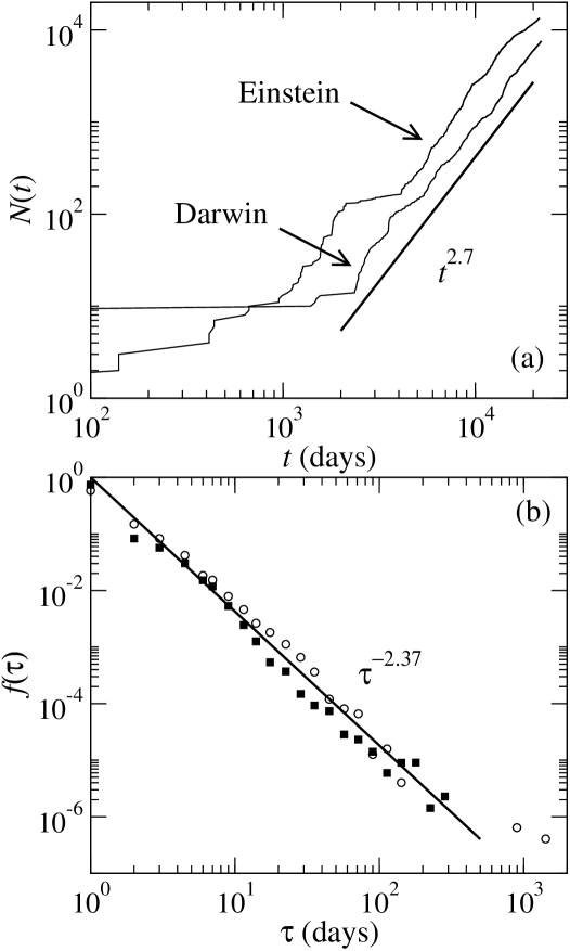
Figure 1: Regular mail activity: Statistical properties of the Darwin’s and Einstein’s correspondence. (a) Cumulative number of letters sent by Darwin (open circles) and Einstein (solid squares). The solid line corresponds with a power law growth $N(t)\sim t^{a}$ with $a=2.7$. (b) The inter-event time distribution associated with the datasets shown in (a). The solid line represents the power law decay $f(\tau)\sim\tau^{-\alpha}$, where the exponent $\alpha$ was obtained using (7) and the value of $a$ obtained from (a).

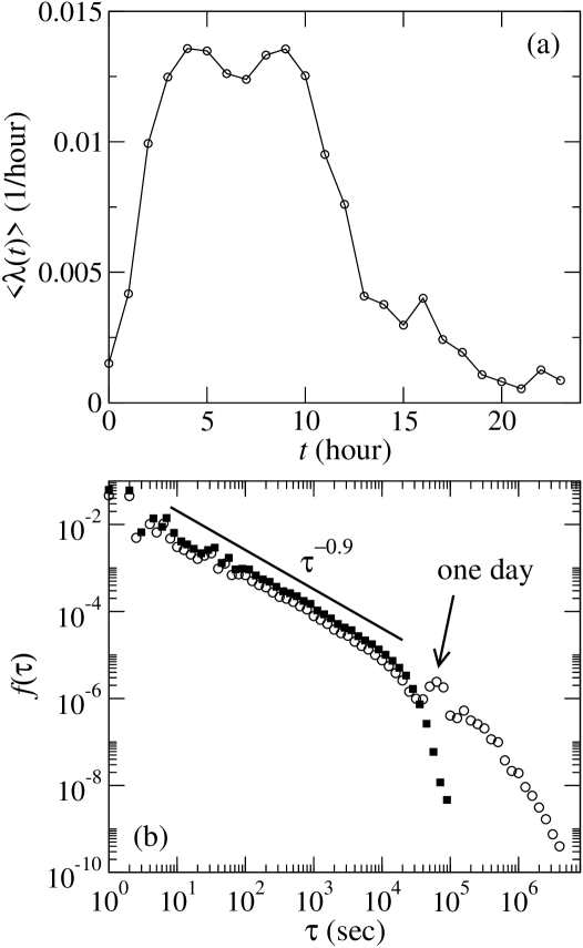
Figure 2: Email activity: Statistical properties of the email activity patterns in an university environment. (a) Email sending rate average over 81 days and 3,188 users as a function of time. The time was shift by a constant such that the start of the working hours corresponds approximately with hour zero. We observe two local maximums associated with the morning and afternoon peaks of daily activity. More importantly, this initial relatively high activity is followed by a reducing tendency. (b) Aggregated inter-event time distribution of all users. The open circles are obtained considering both intra-day and inter-day inter-events, where we can note a local maximum at one day. The solid line represents the power law decay $f(\tau)\sim\tau^{-\alpha}$ with $\alpha=0.9$. The solid squares are obtained considering intra-day inter-events only showing that the power law behavior is determined by intra-day emails.

References

- Anderson (2003) H. R. Anderson, Fixed Broadband Wireless System Design (Wiley, New York, 2003).
- Reynolds (2003) P. Reynolds, Call center staffing (The Call Center School Press, Lebanon, Tenesse, 2003).
- Eubank and et al (2004) S. Eubank and et al, Nature 429, 180 (2004).
- J et al. (2005) G. J, Y. Shavitt, E. Shir, and S. Solomon, Nat. Phys. 1, 184 (2005).
- Hidalgo (2006) C. Hidalgo, Physica A (in press)
- Barabási (2005) A.-L. Barabási, Nature 435, 207 (2005).
- (7) Z. Dezső, E. Almaas, A. Lukács, and A.-L. B. B. Rácz, I. Szakadát, arXive:physics/0505087.
- Oliveira and barabási (2005) J. G. Oliveira and A.-L. barabási, Nature 437, 1251 (2005).
- (9) A. Vazquez, J. G. Oliveira, Z. Dezső, K.-I. Goh, I. Kondor, and A.-L. Barabási, phys. Rev. E (in press).
- Eckmann et al. (2004) J.-P. Eckmann, E. Moses, and D. Sergi, Proc. Natl. Acad. Sci. USA 101, 14333 (2004).