Abstract

We investigate the acceleration of electrons via their interaction with electrostatic waves, driven by the relativistic Buneman instability, in a system dominated by counter-propagating proton beams. We observe the growth of these waves and their subsequent saturation via electron trapping for a range of proton beam velocities, from $0.15c$ to $0.9c$. We can report a reduced stability of the electrostatic wave (ESW) with increasing non-relativistic beam velocities and an improved wave stability for increasing relativistic beam velocities, both in accordance with previous findings. At the highest beam speeds, we find the system to be stable again for a period of $\approx 160$ plasma periods. Furthermore we observe a, to our knowledge, previously unreported secondary electron acceleration mechanism at low beam speeds. We believe that it is the result of parametric couplings to produce high phase velocity ESW’s which then trap electrons, accelerating them to higher energies. This allows electrons in our simulation study to achieve the injection energy required for Fermi acceleration, for beam speeds as low as $0.15c$ in unmagnetised plasma.

fnum@section1 Introduction

Supernova remnant (SNR) shocks, created by the interaction between an expanding supernova blast shell and the ambient medium, are believed to be a significant source of cosmic rays (Reynolds [2001]; Lazendic et al. [2004]), with energies up to $10^{14}$ eV, the knee of the cosmic ray spectrum (Nagano & Watson [2000]; Aharonian et al. [2004]; Völk et al. [1988]).

First order Fermi acceleration has been proposed as a mechanism for the acceleration of electrons to ultra-relativistic velocities in SNR shocks (Bell [1978a]; Bell [1978b]; Blandford & Ostriker [1978]). Electrons gain energy by repeated crossings of the shock front, and by their scattering off MHD waves on either side of the shock. The orientation of the ambient magnetic field $\vec{B}$ relative to the shock normal has implications for the efficiency of electron acceleration (Galeev [1984]). We consider the case where the ambient field is orthogonal to the shock normal, this geometry provides an efficient electron acceleration mechanism for high Mach number shocks (Treumann & Terasawa [2001]). First order Fermi acceleration at such shocks requires a seed population of electrons that have Larmor radii comparable to the shock thickness. Since the shock thickness is, for perpendicular shocks, of the order of the ion Larmor radius, the electrons of this seed population must have mildly relativistic initial speeds. A kinetic energy comparable to 100 keV is believed to be sufficient (Treumann & Terasawa [2001]). Such electrons are unlikely to be present, neither in the interstellar medium (ISM) nor in the stellar wind of the progenitor star of the supernova, but may be created by a pre-acceleration mechanism at the SNR shock front. This pre-acceleration, commonly referred to as the injection problem, is not well understood.

As the shock front of a supernova remnant (SNR) expands into the ISM, it reflects a substantial fraction of the ISM ions as observed in simulations (Shimada & Hoshino [2000]; Schmitz et al. [2002]) and in-situ at the Earth’s bow shock (Eastwood et al. [2005]). If the shock normal is quasi-perpendicular to the magnetic field in a high Mach number shock, as many as 20% of the ions can be reflected (Sckopke et al. [1983]; Galeev [1984]; Lembege & Savoini [1992]; Lembege et al. [2004]). The reflected ions form a beam that can reach a peak speed comparable to twice the shock speed in the ISM frame of reference as, for example, discussed by McClements et al. ([1997]). The shock-reflected plasma particles are a source of free energy, similar to the shock-generated cosmic rays (Zank et al. [1990]) which are also thought to heat the inflowing plasma. However, the shock reflected ion beam is considerably more dense than the cosmic rays and each particle carries less energy. The developing plasma thermalisation mechanisms are thus likely to be different. Since binary collisions between charged particles in the dilute ISM plasma are negligible, these ion beams relax by their interaction with electrostatic waves and electromagnetic waves. In what follows, we focus on the interaction of electrons with high-frequency electrostatic waves (ESWs) that are driven by two-stream instabilities.

Recent particle-in-cell (PIC) simulation studies (Shimada & Hoshino [2003]; Shimada & Hoshino [2004]; Dieckmann et al. [2000]; Dieckmann et al. [2004a]; McClements et al. [2001]) have examined these mechanisms with a particular focus on how and up to what energies the ESWs driven by non-relativistic or mildly relativistic ion beams can accelerate the electrons in the foreshock region.

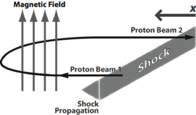
Fig. 1: As the SNR shock expands it reflects a fraction of the ISM protons. These protons move back into the upstream region and form beam 1. The upstream $\vec{B}$ rotates beam 1 which returns as beam 2. The simulation box covers a one dimensional region of x in front of the shock sufficiently small that we can assume it to be spatially homogeneous and one dimensional.

The maximum energy the electrons can reach by such wave-particle interactions, depends on the life-time of the saturated ESW and on the strength and the orientation of $\vec{B}$. Initially a stable non-linear wave known as BGK mode (Bernstein et al. [1957]; Manfredi [1997]; Brunetti et al. [2000]) develops if the plasma is unmagnetised or if the magnetic field is weak (McClements et al. [2001]; Dieckmann et al. [2002]; Eliasson, Dieckmann & Shukla [2005]). Such modes are associated with phase space holes - islands of trapped electrons. These BGK modes are destabilised by the sideband instability, a resonance between the electrons that oscillate in the ESW potential and secondary ESWs (Kruer et al. [1969]; Tsunoda & Malmberg [1989]; Krasovsky [1994]). This resonance transfers energy from the trapped electrons to the secondary ESWs. The initial BGK mode collapses, once these secondary ESWs grow to an amplitude that is comparable to that of the initial wave.

Many previous simulations of two-stream instabilities in the context of electron injection and of shocks have employed PIC simulation codes, which suffer from high noise levels (Dieckmann et al. [2004c]) and from a dynamical range for the plasma phase space distribution that is limited by the number of computational particles. It is thus possible that certain instabilities can not develop, due to a lack of computational particles in the relevant phase space interval, or that the phase space structures (e.g. BGK modes) are destabilised by the noise (Schamel & Korn [1996]) and may benefit from a plasma model based on the direct solution of the Vlasov equation. Such effects have been demonstrated in the non-relativistic limit, for example by Eliasson, Dieckmann & Shukla ([2005]) and Dieckmann et al. ([2004b]), in which the results computed by PIC codes have been compared to those of Vlasov codes. The particle species in a Vlasov code are represented by a continuous distribution function, conventionally evolved on a fixed Eulerian grid, rather than by simulation macro-particles. The comparison of results from these two methodologies has shown significant differences in the life-time of the BGK modes both for unmagnetized and magnetized plasma.

SNR shocks typically expand into the ISM at speeds ranging between a few and twenty percent of $c$ (Kulkarni et al. [1998]). The shock-reflected ions can thus reach a speed of $v_{b}\approx 0.4c$ if the reflection is specular (McClements et al. [1997]) or even higher speeds if we take into account shock surfing acceleration (Ucer & Shapiro [2001]; Shapiro & Ucer [2003]). The proton-beam driven ESWs have a phase speed similar to $v_{b}$ (Buneman [1958]; Thode & Sudan [1973]). Since the ISM electrons can be accelerated to a maximum speed well in excess of the phase speed of the ESW (Rosenzweig [1988]), we must consider relativistic modifications of the life-time of the BGK modes in SNR foreshock plasma. It has been found by Dieckmann et al. ([2004a]) that the BGK mode is stabilised if the phase speed of the ESW is relativistic in the ISM frame of reference. The likely reason is that the change in the relativistic electron mass introduces a strong dependence of the electron bouncing frequency on the electron speed in the ESW frame of reference. This decreases the coherency with which the electrons interact with the secondary ESWs and thus the efficiency of the sideband instability. The stabilization is clearly visible in PIC simulations for ESWs moving with a phase speed of $0.9c$ (Dieckmann et al. [2004a]). For speeds $v_{b}<0.7c$ the relativistic modifications of the BGK mode stability have been small in the PIC simulations (Dieckmann et al. [2004a]). The better representation of the phase space density afforded by a Vlasov simulation may, however, yield a different result and it requires a further examination.

We thus focus in this work on the modelling of electrostatic instabilities by means of relativistic Vlasov simulations and we assess the impact of these instabilities as a potential pre-acceleration mechanism. To this end, we neglect magnetic field effects and consider only the one-dimensional electrostatic system, which is equivalent to the approach taken by Dieckmann et al. ([2004a]) but at a much larger dynamical range for the plasma phase space distribution. This description serves as simple model for the stability of ESWs by which we identify similarities and differences between the results provided by PIC and Vlasov simulations. Future work will expand the simulations to include magnetic fields, which introduces electron surfing acceleration (ESA) (Katsouleas & Dawson [1983]; McClements et al. [2001]) and stochastic particle orbits (Mohanty & Naik [1998]), and multiple dimensions.

More specifically, we examine by relativistic electrostatic Vlasov simulations (Arber & Vann [2002]; Sircombe et al. [2005]) how the BGK mode life-time and its collapse in an unmagnetised plasma depend on $v_{b}$ and thus on the phase speed of the ESW. The purpose is twofold. First, we extend the comparison of results provided by PIC and by Vlasov codes beyond the nonrelativistic regime in Dieckmann et al. ([2004b]). We perform Vlasov simulations for initial conditions that are identical to those in Dieckmann et al. ([2004a]) where a PIC simulation code (Eastwood [1991]) has been used. We find a good agreement of the results of the relativistic Vlasov code and the PIC code for relativistic $v_{b}$ and with the corresponding result provided by the nonrelativistic Vlasov code (Eliasson [2002]; Dieckmann et al. [2004b]). We thus bring forward further evidence for both, an increasing destabilisation of BGK modes for increasing nonrelativistic phase speeds of the wave and a stabilisation for increasing relativistic phase speeds. Secondly we want to exploit the much higher dynamical range of Vlasov simulations to examine the wave spectrum and the particle energy spectrum that we obtain by the considered nonlinear interactions. We find that the collapse of the BGK modes couples energy to three families of waves. Firstly a continuum of electrostatic waves that move with approximately the beam speed. These waves are connected to the turbulent electron phase space flow. Secondly we find for high beam speeds the growth of quasi-monochromatic modes with frequency comparable to the Doppler-shifted bouncing frequency of the trapped electrons in the wave potential. These waves would be sideband modes (Kruer et al. [1969]). Thirdly we find waves that do not have a clear connection to any characteristic particle speed. We believe that these modes are produced by parametric instabilities. These modes can reach phase speeds well above the maximum speed the initial trapped electron population reaches, and they grow to amplitudes at which they can trap electrons, i.e. a BGK mode cascade to high speeds develops. By this trapping cascade, the electrons can reach momenta well in excess of those reported previously (Dieckmann et al. [2000]; Dieckmann et al. [2004a]). This result would imply that the ion beams, that are reflected by shocks that expand at speeds comparable to SNR shocks, can accelerate electrons to energies in excess of 100 keV, at which they can undergo Fermi acceleration to higher energies.

fnum@section2 The physical model, the linear instability and the simulation setup

fnum@subsection2.1 Physical model

We consider a small interval of the ISM plasma just ahead of the SNR shock (see Fig. 1) and we treat the ISM plasma as an electron proton plasma with a spatially homogeneous Maxwellian velocity distribution. We place our simulation box close to the SNR shock, so that the shock-reflected ISM protons can cross it. The protons, that have just been reflected, constitute beam 1, beam 2 represents the protons that return to the shock after they have been rotated by the global foreshock magnetic field. Our model is in line with that discussed, for example, by McClements et al. ([1997]) and solved numerically, e.g. for unmagnetized plasma by Dieckmann et al. ([2000, 2004a, 2004b]) and for magnetized plasma by McClements et al. ([2001]) and by Shimada & Hoshino ([2004]).

We set $\vec{B}=0$, and thus, exclude electromagnetic instabilities, e.g. Whistler waves (Kuramitsu & Krasnoselskikh [2005]), MHD waves, and electrostatic waves in magnetised plasma, e.g. electron cyclotron waves. However, by this choice we decouple the development of competing instabilities and we can consider them separately. In this work we focus on ESWs and the nonlinear BGK modes, which are important phase space structures in the foreshocks of Solar system plasma shocks (Treumann & Terasawa [2001]).

The system is, with the choice $\vec{B}=0$, suitable for modelling with an electrostatic and relativistic Vlasov-Poisson solver. The size of the simulation box is small compared to the distance across which the beam parameters change. Thus we can take periodic boundary conditions for the simulation and spatially homogeneous Maxwellian distributions for both beams. Both beams have the same mean speed modulus, $|v_{b}|$, but move into opposite directions which gives a zero net current in the simulation box. We take a higher temperature for beam 2 than for beam 1 to reflect the scattering of the beam protons as they move through the foreshock. We show the velocity distributions in Fig. 2

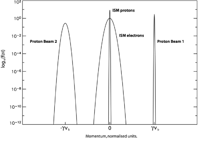
Fig. 2: The initial velocity distribution showing the ISM electrons and protons, proton beam 1 and proton beam 2. The expanding SNR shock reflects a fraction of the ISM protons which form beam 1. The upstream $\vec{B}$ rotates beam 1 to create beam 2. Since the beam has been scattered by ESWs on its path through the foreshock, its thermal spread has increased. Both beams can grow ESWs with a speed similar to $v_{b}$ which saturate by their interaction with the ISM electrons. By assuming that the plasma parameters do not change over the small box size we consider, we can represent this plasma by the 4 spatially homogeneous species shown.

The choice of $\vec{B}=0$ is a critical limitation of the model. The initial conditions described above could not fully describe a perpendicular shock and with $\vec{B}=0$ one could not account for the presence of a returning proton beam. We assume that, while the field is neglected over the simulation box, the field outside the box is sufficient to produce the proton beam structure described. Therefore, the results presented here are not directly applicable to the foreshock dynamics of high Mach number shocks. However, they provide an overview of processes that require a large dynamical range for the plasma phase space distribution and which may, therefore, not have been observed in previous PIC simulations. Our system is applicable to parts of the foreshock of perpendicular shocks, where magnetic field fluctuations (Jun & Jones [1999]) cause the magnetic field to vanish or to be beam aligned. It may also apply to the field aligned ion beams that are observed in the foreshock region of the Earth’s bow shock (Eastwood et al. [2005]) and which may be present also at SNR shocks. Here, the second proton beam in our initial conditions takes the role of the return current in the plasma which is typically provided by all plasma species (Lovelace & Sudan [1971]). Interactions between two BGK modes in unmagnetized plasma affect primarily the velocity interval that is confined by the phase speeds of the two waves (Escande [1982]). Our results, which focus on the developing high energy tails of the plasma distribution, may thus not depend on the exact setting of the initial return current and may be more universally applicable.

fnum@subsection2.2 Linear instability

We introduce the plasma frequency of each species $i$ as $\omega_{p,i}={(e^{2}n_{i}/m_{i}\epsilon_{0})}^{1/2}$ where $e$, $n_{i}$, $m_{i}$ and $\epsilon_{0}$ are the magnitude of the elementary charge, the number density of species $i$ in the rest frame of the species, the particle mass of species $i$ and the dielectric constant. In what follows we define all $\omega_{p,i}$ in the box frame of reference. Species 1 and 2 are the ISM electrons and protons. The species 3 is beam 1 and species 4 is beam 2. The large inertia of species 2 compared to species 1 implies, that its contribution to the linear dispersion relation can be neglected. The linear dispersion relation then becomes in the cold plasma limit

$$\frac{\omega_{p,1}^{2}}{\omega^{2}}+\frac{\omega_{p,3}^{2}}{\gamma^{3}(v_{b}){(\omega-v_{b}k)}^{2}}+\frac{\omega_{p,4}^{2}}{\gamma^{3}(v_{b}){(\omega+v_{b}k)}^{2}}-1=0$$ (1)

During the linear growth phase, each proton beam will grow an ESW by its streaming relative to the electrons. Both waves are well separated in their phase speed and the linear dispersion relation can be solved separately for each ESW by neglecting either the term with $\omega_{p,3}$ or $\omega_{p,4}$ in Eq. 1 (Buneman [1958]; Thode & Sudan [1973]). Its frequency in the box frame is $\omega_{u}\approx\omega_{p,1}$, its wave number is $k_{u}\approx\omega_{p,1}v_{b}^{-1}$ and its growth rate is $\Omega\approx{(3\sqrt{3}\omega_{p,3}^{2}\omega_{p,1}/16)}^{1/3}/\gamma(v_{b})$. We take a number density ratio of $n_{3}/n_{1}=0.2\gamma(v_{b})$ and set $n_{4}=n_{3}$ and $n_{2}=n_{1}-n_{3}-n_{4}$ in the box frame of reference, which is representative for a shock with a high Mach number (Galeev [1984]). This density ratio gives $\omega_{p,1}/\omega_{p,3}\approx 96{\gamma(v_{b})}^{-0.5}$ and a growth rate of $\Omega\approx 0.033/{\gamma(v_{b})}^{2/3}$. The growth rate is reduced by increasing temperatures of the plasma. The wave length of the most unstable ESW is $\lambda_{u}=2\pi/k_{u}$. The sideband instability couples energy to modes with $k\leq k_{u}$, for non-relativistic phase speeds of the wave (Krasovsky [1994]). We thus set the simulation box length to $L=2\lambda_{u}$ to resolve more than one unstable sideband mode, which leads to a wave collapse (Dieckmann et al. [2000]).

This $L$ is short compared to the typical size of the foreshock which justifies our spatially homogeneous initial conditions and periodic boundary conditions. We use the amplitudes of the initial ESW and that of the sideband modes as indicators for the wave collapse. We define $l$ as the index of the simulation cell, $x_{l}=l\Delta x$, $k_{j}=2\pi j/N_{x}\Delta x$ and $N_{x}$, as the number of simulation cells in $x$. The index $m$ refers to the data time step $m\Delta t$, where $\Delta t$ is the time interval between outputs rather than the simulation time step. We Fourier Transform the spatio-temporal ESW field $E(x,t)$ as

$$E(k_{j},t_{m})=\left[{N_{x}}^{-1}|\sum_{l=1}^{N_{x}}E(x_{l},t_{m})\exp{(ik_{j}x_{l})}|\right]$$ (2)

The amplitude of the ESW with $k=k_{u}$ at the simulation time $t_{m}$ is then given by $E(k_{2},t_{m})$.

To analyse the nonlinear and time dependent processes developing after the saturation of the ESW, we introduce a Window Fourier Transform. We define the window size, in time steps, as $N_{t}$ and we introduce $\omega_{n}=n\Delta\omega=n(2\pi/N_{t}\Delta t)$ as the frequency defined in a Fourier time window with a size $N_{t}\Delta t$. This frequency is limited by the sampling theorem to $-\pi/\Delta t<\omega_{n}\leq\pi/\Delta t$. The Window Fourier transform can be written as

$$W_{1}(k_{j},t_{m}) = {N_{x}}^{-1}\sum_{l=1}^{N_{x}}E(x_{l},t_{m})\exp{(ik_{j}x_{l})}$$

$$W_{2}(\omega_{n},t_{s},k_{c}) = {N_{t}}^{-2}{\left|{\sum_{l=s-N_{t}/2+1}^{s+N_{t}/2}W_{1}(k_{c},t_{l})}\exp{(i\omega_{n}t_{l})}\right|}^{2}$$ (3)

where the Fourier transformed time interval is small compared to the total length of the time series, which is $19N_{t}\Delta t$, and where $k_{c}$ is a fixed wave number.

fnum@subsection2.3 Numerical Simulation

In the absence of a magnetic field the one dimensional relativistic Vlasov-Poisson system of electrons and protons is given by the Vlasov equation for the electron distribution function $f_{e}(x,p,t)=f_{1}$

$$\frac{\partial f_{e}}{\partial t}+\frac{p}{m_{e}\gamma}\frac{\partial f_{e}}{\partial x}-eE\frac{\partial f_{e}}{\partial p}=0,$$ (4)

the Vlasov equation for the proton distribution function $f_{p}(x,p,t)=f_{2}+f_{3}+f_{4}$

$$\frac{\partial f_{p}}{\partial t}+\frac{p}{m_{p}\gamma}\frac{\partial f_{p}}{\partial x}+eE\frac{\partial f_{p}}{\partial p}=0,$$ (5)

and Poisson’s equation for the electric field

$$\frac{\partial E}{\partial x}=-\frac{e}{\epsilon_{0}}\left(\int f_{e}dp-\int f_{p}dp\right)$$ (6)

The Vlasov-Poisson system is solved using a parallelised version of the code detailed in Arber & Vann ([2002]) and Sircombe et al. ([2005]). This uses a split Eulerian scheme in which the distribution functions ($f_{e},f_{p}$) are calculated on a fixed Eulerian grid. The solver is split into separate spatial and momentum space updates (Cheng & Knorr [1976]). These updates are one dimensional, constant velocity advections carried out using the piecewise parabolic method (Colella & Woodward [1984]).

fnum@subsection2.4 Initial Conditions

Throughout our simulations we adopt a realistic mass ratio, $m_{p}/m_{e}=M_{r}$, of $M_{r}=1836$ and resolve $L$ by 512 cells in the $x-$direction, each with length $\Delta x=\pi v_{b}/128\omega_{p,1}$. To accurately resolve the filamented phase space distributions of the particles that result from the sideband instability (McClements et al. [2001]), we use a momentum-space grid with between 4096 and 16384 grid points ($N_{p}$). This ensures that the momentum grid spacing for each species, $\Delta p_{x,i}$, is small. Specifically, $\Delta p_{x,i}<0.1m_{i}v_{th,i}$ where $v_{th,i}^{2}=\kappa T_{i}/m_{i}$ is the thermal speed of species $i$ and where $\kappa$ and $T_{i}$ are the Boltzmann constant and the temperature of species $i$.
We set the temperatures of the four species to $T_{1}=5.4\times 10^{5}$ K, $T_{2}=T_{3}=10T_{1}$ and $T_{4}=100T_{2}$. We thus obtain $v_{th,1}=10^{-2}c$. Each species is described by a Maxwellian momentum distribution of the form

$$f_{i}(p)=C_{i}\exp\left(\frac{-m_{i}\left(\gamma(p-p_{0})-1\right)}{T_{i}}\right)$$ (7)

where $p_{0}$ is the initial momentum offset, zero for species 1 and 2, $\pm v_{b}/(1-v_{b}^{2}/c^{2})^{0.5}$ for species 3 and 4 respectively. For each species the constant $C_{i}$ is calculated to ensure that $\int f_{i}dp=n_{i}$ and that $\int\left(f_{2}+f_{3}+f_{4}\right)dp=n_{1}$, so there is no net charge in the system.
In order to excite the linear instability, we add to the proton distribution (species 2, 3 and 4) a density perturbation at the most unstable wavenumber of the form $n^{\prime}=a\cos{k_{u}x}$, where $a$ is small, typically of the order of 1% of the background density. The minimum beam speed of $v_{b}=0.15c$ we examine here corresponds to the slow beam in Dieckmann et al. ([2004b]). The maximum beam speed $v_{b}=0.9c$ equals the maximum beam speed in Dieckmann et al. ([2004a]).

fnum@section3 Simulation results

Simulations use a system of normalised units where time is normalised to $\omega_{p,1}^{-1}$, space to $c\omega_{p,1}^{-1}$ and momenta to $\gamma m_{e}c$. It follows that the electric field is normalised to $\omega_{p,1}cm_{1}/e$. Where appropriate in the figures, we re-normalise $x$ in units of $2\pi/k_{u}$, the most unstable wavelength for a given initial beam speed. This ensures that the spacial units are identical for all beam speeds.

fnum@subsection3.1 Growth and non-linear Saturation of the Buneman instability

Figure 3 shows the initial growth stage of the most unstable mode, $E(k=k_{u})$, for a range of initial beam velocities. From these we estimate the growth rate of the instability ($\Omega$), in normalised units, to be $0.0256,0.0264,0.0270,0.0246,0.0201$ and $0.0137$ for beam speeds of $v_{b}=0.15c,0.2c,0.4c,0.6c,0.8c$ and $0.9c$, respectively. These compare favourably with the linear theory. Writing $\alpha(v_{b})$ as the ratio between observed and theoretical growth rates we find; $\alpha(0.15c)\approx 0.79$, $\alpha(0.2c)\approx 0.81$, $\alpha(0.4c)\approx 0.87$, $\alpha(0.6c)\approx 0.87$, $\alpha(0.8c)\approx 0.86$ and $\alpha(0.9c)\approx 0.72$. As explained in Dieckmann et al. ([2004a]), where a similar systematic reduction has been observed in PIC simulations (in this case by 15-20%), this might be connected with the fast growth rate of the instability itself since it results in a considerable spread in frequency for the unstable wave. This makes the treatment of the instability in terms of single frequencies ($\omega_{u}$) inaccurate. In truth, the growth rate should be lower since the energy of the unstable wave is spread over damped frequencies.

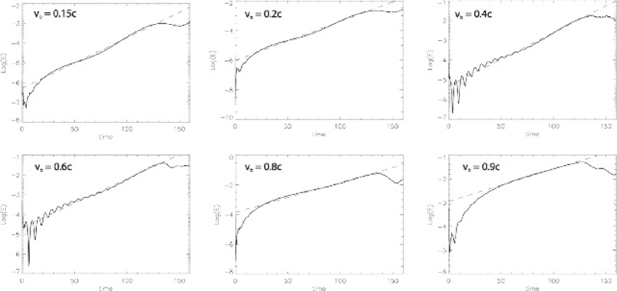
Fig. 3: The logarithmic amplitude of the most unstable mode $E(k_{u},t)$ is plotted against time, in normalised units, for a variety of beam speeds. The dashed lines on each plot represent a linear fit over the region of exponential growth. Using this linear fit we obtain growth rates for the relativistic Buneman instability, in normalised units, of $\Omega\approx 0.0256,0.0264,0.0270,0.0246,0.0201$ and $0.0137$ for beam speeds of $v_{b}=0.15c,0.2c,0.4c,0.6c,0.8c$ and $0.9c$, respectively.

The ESWs saturate by the trapping of electrons and the formation of BGK modes. This is shown in Fig. 4, for the case of $v_{b}=0.2c$, and Fig. 5 for $v_{b}=0.9c$. Here we see the appearance of phase-space holes characteristic of particle trapping. While the saturation mechanism is the same in both cases, for the high velocity beam we observe the development of two counter-propagating BGK modes. This is because at lower beam speeds the ESW instability driven by the cooler beam (at $+v_{b}$) dominates whereas for higher, relativistic, beam speeds forwards and backwards propagating ESWs grow in unison. At lower beam speeds the increased temperature of beam 2 (species 4) is more significant, since the thermal velocity of the beam is a larger proportion of the beam speed than is the case at $v_{b}=0.9c$. Thus, the growth rate for the hot beam is sufficiently reduced for the system to be dominated by the growth of the cooler proton beam (species 3). We do observe the growth of a counter propagating ESW which begins to trap electrons after $t=150$. However, the final momentum distribution is clearly dominated by electrons accelerated by the ESW with positive phase velocity. At $v_{b}=0.9c$, the thermal spread of both proton beams is negligible in comparison to the beam velocities and we observe the growth and saturation of ESWs associated with both beams.

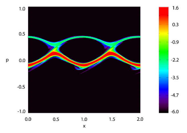
Fig. 4: Contour plot of $\log(f_{e}>10^{-6})$ at time $t=150$ for a system with an initial beam velocity of $v_{b}=0.2c$. The exponential growth of the ESW is in the process of saturating via the trapping of electrons, forming a BGK mode at $p\approx+0.2.$. The thermal spread of beam 2 inhibits its growth slightly, allowing the system to become dominated by one ESW. Hence, we do not observe electron trapping around $p\approx-0.2$. Here $x$ is given in units of $2\pi/k_{u}$.

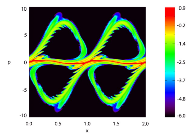
Fig. 5: Contour plot of $\log(f_{e}>10^{-6})$ at time $t=200$ for a system with a relativistic initial beam velocity of $v_{b}=0.9c$. The exponential growth of the ESW is in the process of saturating via the trapping of electrons, forming a pair of BGK modes at $p\approx\pm 3$. The reduced significance of the higher temperature of species 4, with respect to species 3, at high beam speeds allows the growth of forwards and backwards propagating ESWs simultaneously. Here $x$ is given in units of $2\pi/k_{u}$.

fnum@subsection3.2 Wave collapse and secondary electron trapping

Trapping of electrons in electrostatic waves produces BGK modes which eventually collapse via the sideband instability. The sideband instability is due to the nonlinear oscillations of the electrons in the potential of the ESW. For electrons close to the bottom of the wave potential, their oscillation is that of a harmonic oscillator. The monochromatic bouncing frequency is Doppler shifted, due to the phase speed of the ESW. These sidebands can couple the electron energy to secondary high-frequency ESWs, which must have a wave number $k\leq k_{u}$ (Krasovsky [1994]). The sideband instability is a limiting factor for the lifetime of the ESW which has implications in the presence of an external magnetic field in particular. To demonstrate this we show in Fig. 6 the amplitude of the ESW driven by beam 1 at $k=k_{u}$ for beam speeds ranging from $0.15c$ to $0.9c$. We find that the ESWs moving at nonrelativistic phase speeds saturate smoothly, which is in line with the wave saturation of the ESW in the Vlasov simulation in Dieckmann et al. ([2004b]). Their lifetime is significant and, in the presence of a weak external magnetic field $\vec{B}$ orthogonal to the wave vector $\vec{k}$, the trapped electrons would undergo substantial ESA (Eliasson, Dieckmann & Shukla [2005]). The ESA is proportional to $v_{ph}|\vec{B}|$ and the comparatively low $v_{ph}$ would limit the maximum energy the electrons can reach.

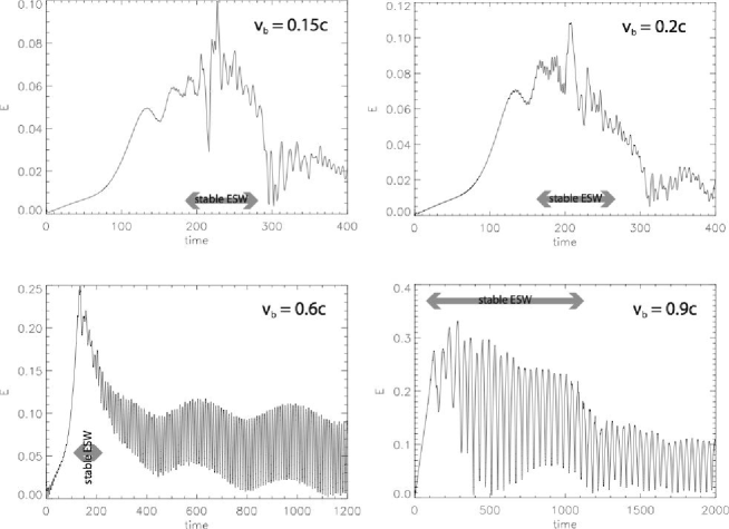
Fig. 6: The time evolution of the ESW amplitudes with $k=k_{u}$ that are driven by beam 1 for beam speeds of $0.15c$, $0.2c$, $0.6c$ and $0.9c$. ESWs generated at non-relativistic beam speeds saturate smoothly and stabilise briefly. At $v_{b}=0.6$ the ESW collapses abruptly and at relativistic beam speeds, $v_{b}=0.9c$ we observe a stabilisation of the ESW for a period of almost $1000\omega_{pe}^{-1}$, equivalent to almost $160$ plasma periods. Approximate regions of stability are highlighted on each plot.

The ESW driven by the beam with $v_{b}=0.6c$ grows to a larger amplitude and then collapses abruptly, which confirms the finding in Dieckmann et al. ([2004b]) that the BGK modes become more unstable the larger the ratio between beam speed to electron thermal speed becomes. The Lorentz force $ev_{ph}|\vec{B}|$ excerted by a $\vec{B}\bot\vec{k}$ would be significantly higher than for the case $v_{b}=0.15$, however the short lifetime of the wave would here prevent electrons from reaching highly relativistic speeds. By increasing the beam speed to $v_{b}=0.9c$ we obtain a stabilisation of the ESW, in line with the results in Dieckmann et al. ([2004a]). Here the Lorentz force is strong and the lifetime of the saturated ESW is long constituting a formidable electron accelerator, provided the field evolution is not strongly influenced by $\vec{B}$.

We now summarise the principal results from each beam speed. Note that in particular the ESWs driven by the mildly relativistic proton beams show oscillations after their initial saturation. To identify the origin of these fluctuations we apply a Window Fourier Transform to the amplitudes of the ESWs with the wavenumbers $k_{u}/2$ and $k_{u}$.

fnum@subsection3.3 Beam speed, $v_{b}=0.15c$.

In Fig. 7 we find a strongly asymmetric ESW growth for $v_{b}=0.15c$. Here the thermal spread of the individual plasma species is not small compared to $v_{b}$. Therefore the ESW driven by the cooler beam 1 grows and saturates first. It rapidly collapses and this collapse inhibits a further growth of the ESW driven by beam 2. The initial monochromatic ESW collapses into a broad wave continuum centred around $\omega=\omega_{p,1}$. We find the equivalent broad wave continuum for $k=k_{u}/2$ centred at $\omega=\omega_{p,1}/2$. These waves propagate at phase speeds comparable to $v_{b}$ and represent the structures remaining of the initial BGK mode. The ESW spectrum at $k=k_{u}/2$ further shows two wave bands that are separated by a frequency of $\omega_{p,1}$ from the main peak. These two wave bands could be pumped by a beat between the turbulent structure centred at $\omega=\omega_{p,1}/2$, $k=k_{u}/2$, the turbulent structure centred at $\omega=\omega_{p,1}$ and $k=k_{u}$ and the Langmuir wave with $k=k_{u}/2$. Evidence for this is the correlation between both turbulent structures and the wave bands at $t\approx 2500$. At this time most wave power at $\omega\approx\omega_{p,1}/2$ is absorbed at $k\approx k_{u}/2$. At the same time wave power at $\omega\approx\omega_{p,1}$ is absorbed at $k=k_{u}$ while the power in the wave bands with $\omega\approx\omega_{p,1}/2$ and $\omega\approx 1.5\omega_{p,1}$ grows at $k=k_{u}/2$. The faster of these two has a phase speed of $\omega/k\approx 3v_{b}=0.45c$.

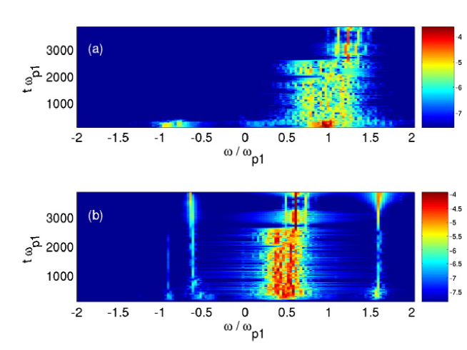
Fig. 7: The ESW spectrum for a beam speed of $v_{b}=0.15c$: (a) shows the frequency power spectrum of $k_{c}=k_{u}$ and (b) shows the frequency power spectrum of $k_{c}=k_{u}/2$ as a function of time. The colour scale shows $\log_{10}W_{2}(\omega,t,k_{c})$. The ESW driven by beam 1 with $v_{b}>0$ corresponds to the wave with $\omega=\omega_{p,1}$ in (a).

This beat wave is thus considerably faster than the initial ESW. By its large amplitude it could trap electrons. This is confirmed by Fig. 8 where we find a BGK mode in the electron distribution centred around a momentum $p/m_{e}c\approx 0.52$ which corresponds to a speed $0.46c$. The fastest electrons of this BGK mode reach $p/m_{e}c\approx 0.68$ or a speed of $0.56c\approx 3.75v_{b}$.

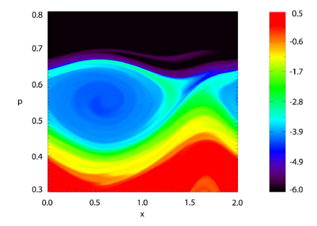
Fig. 8: Contour plot of $\log(f_{e}>10^{-6})$ for $v_{b}=0.15c$ at the time $t=3500$: The initial electron BGK modes have collapsed and they can be shown to form a plateau distribution at $p/m_{e}c<0.3$. Centred at $p/m_{e}c\approx 0.52$ we find BGK modes driven by the beat wave.

fnum@subsection3.4 Beam speed, $v_{b}=0.2c$.

The simulation with $v_{b}=0.2c$ shows a similar wave coupling as shown in Fig. 9. We find a turbulent ESW spectrum that has been driven by the beam 1 and that covers waves with phase speeds centred at $v_{b}$ with a spread that is a significant fraction of the beam speed. Initially an ESW is also driven by beam 2 at $\omega\approx\omega_{p,1}$ but, in line with Fig. 7, it collapses simultaneously with the ESW driven by beam 1. The turbulent wave spectrum with $\omega\approx\omega_{p,1}$ at $k=k_{u}$ appears to couple with the equivalent spectrum at $\omega\approx\omega_{p,1}/2$ at $k=k_{u}/2$ and the Langmuir wave with $\omega=\pm\omega_{p,1}$ and $k=k_{u}/2$ to give wave bands at $\omega\approx-0.5\omega_{p,1}$ and at $\omega\approx 1.5\omega_{p,1}$. The phase speed of the ESW band at $\omega\approx 1.5\omega_{p,1}$ is $\omega/k\approx 3v_{b}$ and that of the band at $\omega\approx\omega_{p,1}/2$ is $\omega/k\approx v_{b}$.

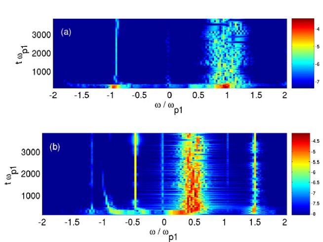
Fig. 9: The ESW spectrum for a beam speed of $v_{b}=0.2c$: (a) shows the frequency power spectrum of $k_{c}=k_{u}$ and (b) shows the frequency power spectrum of $k_{c}=k_{u}/2$ as a function of time. The colour scale shows $\log_{10}W_{2}(\omega,t,k_{c})$. The ESW driven by beam 1 with $v_{b}>0$ corresponds to the wave with $\omega=\omega_{p,1}$ in (a).

The large amplitudes of both bands suggests that they might also be trapping electrons. This is confirmed by Fig. 10 where we show the electron momentum distribution at $t=2000$. We find BGK modes centred at $p/m_{e}c\approx 0.75$ or a speed of 0.6c. The BGK modes extend up to a peak momentum of $p/m_{e}c\approx 1$ or a speed of 0.87c respectively equivalent to $4.5v_{b}$.

Fig. 10: Contour plot of $\log(f_{e}>10^{-6})$ for $v_{b}=0.2c$ at the time $t=2000$: The initial electron BGK modes have collapsed and form a plateau distribution. Centred at $p/m_{e}c\approx 0.75$ we find BGK modes driven by the beat wave.

fnum@subsection3.5 Beam speed, $v_{b}=0.4c$.

As we increase the beam speed to $v_{b}=0.4c$ the ESW driven by beam 1 stabilises and the collapsing ESW driven by beam 2 drives the broadband turbulence as we see from Fig. 11. The peak energy of the two counter-propagating ESWs is now comparable. Since we keep the thermal spread of the beams constant while increasing $v_{b}$, the thermal effects are reduced and the growth rate of both waves approaches the peak growth rate for the cold beam instability. We find the growth of ESWs at $k=k_{u}$ with $|\omega|\approx 2\omega_{p,1}$. Since these ESWs have the same wave number as the initial wave they can not be produced by self-interaction of the initial ESW since this would also double the wave number. Instead we believe that these high frequency waves correspond to the Doppler shifted bouncing frequency of the trapped electrons in the potential of the strong ESW. The fastest electrons reach approximately twice the phase speed $v_{ph}$ of the ESW as can be seen, for example, at the lower beam speed of $v_{b}=0.2c$ in Fig. 4. These electrons are thus, due to the fixed wave number $k_{u}$ of the BGK modes, interacting with secondary ESWs with $\omega\approx 2\omega_{p,1}$. The ESWs with $|\omega|\approx 1.2\omega_{p,1}$ at $k=k_{u}/2$ are, on the other hand, possibly due to a beat between the ESWs with $|\omega|=\omega_{p,1}$ at $k=k_{u}$ and the ESWs with $|\omega|=\omega_{p,1}/2$ at $k=k_{u}/2$ and Langmuir waves, as for the slower ESWs.

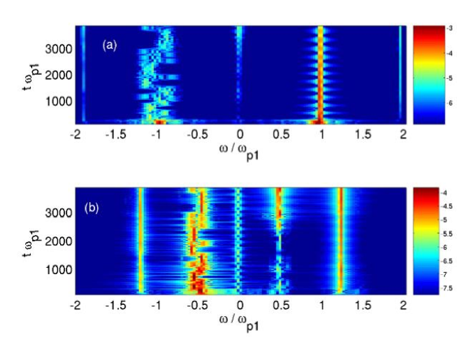
Fig. 11: The ESW spectrum for a beam speed of $v_{b}=0.4c$: (a) shows the frequency power spectrum of $k_{c}=k_{u}$ and (b) shows the frequency power spectrum of $k_{c}=k_{u}/2$ as a function of time. The colour scale shows $\log_{10}W_{2}(\omega,t,k_{c})$. The ESW driven by beam 1 with $v_{b}>0$ corresponds to the wave with $\omega=\omega_{p,1}$ in (a).

fnum@subsection3.6 Beam speed, $v_{b}=0.6c$.

The ESW wave spectrum for $v_{b}=0.6c$ is similar to that for $v_{b}=0.4c$. Again we find that both beams grow strong ESWs close to $|\omega_{u}|=\omega_{p,1}$ but that it is the still stronger ESW driven by beam 1 that stabilises while that driven by beam 2 collapses into a broadband spectrum. This is also reflected by the ESW spectrum at $k_{u}/2$ where we find the strongest wave activity at $\omega\approx-\omega_{p,1}/2$. Two additional wave bands with frequencies $\omega\approx\omega_{p,1}$ are observed at $k_{u}/2$, i.e. long Langmuir waves are produced by the nonlinear processes. These waves have twice the phase speed of the initial ESWs and by their superluminal phase speed they can not interact resonantly with the electrons. At $k=k_{u}$, on the other hand, we find high-frequency modes at $|\omega|\approx 1.6\omega_{p,1}$ with a subluminal phase speed $\omega/k_{u}\approx 0.95c$.

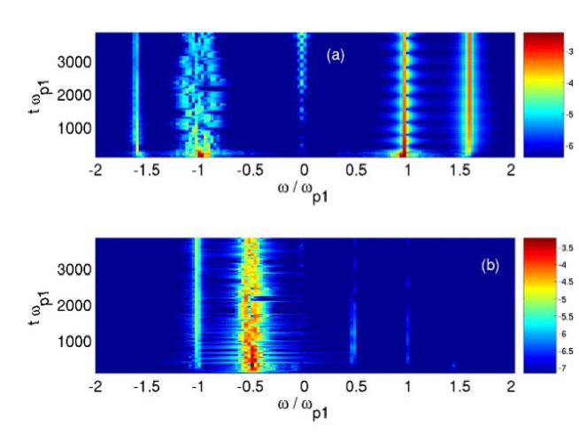
Fig. 12: The ESW spectrum for a beam speed of $v_{b}=0.6c$: (a) shows the frequency power spectrum of $k_{c}=k_{u}$ and (b) shows the frequency power spectrum of $k_{c}=k_{u}/2$ as a function of time. The colour scale shows $\log_{10}W_{2}(\omega,t,k_{c})$. The ESW driven by beam 1 with $v_{b}>0$ corresponds to the wave with $\omega=\omega_{p,1}$ in (a).

The phase speeds of these ESWs is higher than the peak speed the electrons reach in the inital BGK mode as shown in Fig. 13. We can thus not explain its growth by a streaming instability between the trapped electrons and, for example, the untrapped electrons. We can obtain phase speeds of the ESW bands that are higher than the speed of the trapped electron beam, however, by applying the relativistic Doppler shift to the electron bouncing frequency in the ESW wave potential. The rest frame of the ESWs moves with the speed $v_{ph}=0.6c$. The frequency of the ESWs in the observer frame is, according to Fig. 12, $\omega_{o}\approx 1.6\omega_{p,1}$. With the relativistic Doppler equation we would obtain a bouncing frequency of the electrons in the ESW frame of reference of $\omega_{b}={([1-v_{ph}/c]/[1+v_{ph}/c])}^{1/2}\omega_{o}=0.8\omega_{p,1}$. We use the nonrelativistic estimate of the electron bouncing frequency in a parabolic electrostatic potential $\omega_{b}^{2}=ek_{u}E/m_{e}$ and the corresponding width of the trapped electron island $v_{tr}^{2}=2eE/m_{e}k_{u}$ to eliminate the electric field $E$. We obtain the relation $\omega_{b}/k_{u}=v_{tr}/\sqrt{2}$. Since for our cold plasma species the velocity width of the island of trapped electrons must be comparable to $v_{ph}$ to trap the bulk electrons we get an estimate for $\omega_{b}\approx\omega_{p,1}/\sqrt{2}$ which is close to $\omega_{o}$. We may thus indeed interpret the two sidebands observed in Fig. 12 as the Doppler shifted bouncing frequency of the electrons.

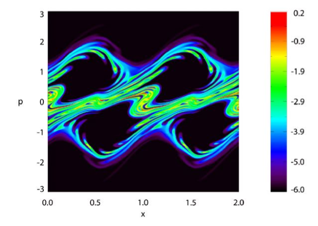
Fig. 13: Contour plot of $\log(f_{e}>10^{-6})$ for $v_{b}=0.6c$ at the (early) time $t=200$: The initial electron BGK modes have just been formed and the trapped electrons reach a momentum up to $p/m_{e}c\approx 3$.

These sideband modes driven by the beams of trapped electrons have a phase speed that is just below $c$ and a large amplitude. Since their phase speed is comparable to the fastest speed the electrons reach in the initial BGK mode, they should be capable of trapping some of these electrons. This is confirmed by Fig. 14 where we find BGK modes centred at the momentum $p/m_{e}c\approx 3.4$ which accelerate electrons up to the peak momentum $p/m_{e}c\approx 7$ or a speed of $0.99c$.

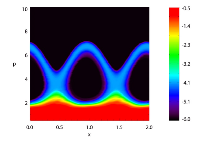
Fig. 14: The electron momentum distribution for $v_{b}=0.6c$ at the (late) time $t=3500$: The initial electron BGK modes have collapsed and the electrons that are trapped by the sideband mode reach a momentum up to $p/m_{e}c\approx 7$.

fnum@subsection3.7 Beam speed, $v_{b}=0.8c$ and $v_{b}=0.9c$.

As we increase the beam speed to $v_{b}=0.8c$ the qualitative evolution of the ESWs changes. At this high beam speed the thermal spread of the plasma species is negligible. The growth rates of the waves for both beams is approximately that of the cold beam instability and the ESWs grow symmetrically. Both saturated ESWs are stable. After the saturation each ESW shows a sideband, similar to that in Fig. 13 at a frequency modulus $\omega\approx 1.3\omega_{p}$. The phase speeds of these sideband modes are presumably just above $c$. We find a growing second mode at $k=k_{u}/2$ at the frequency modulus $\omega\approx 0.8\omega_{p,1}$ which moves at a superluminal phase speed.

Fig. 15: The ESW spectrum for a beam speed of $v_{b}=0.8c$: (a) shows the frequency power spectrum of $k_{c}=k_{u}$ and (b) shows the frequency power spectrum of $k_{c}=k_{u}/2$ as a function of time. The colour scale shows $\log_{10}W_{2}(\omega,t,k_{c})$. The ESW driven by beam 1 with $v_{b}>0$ corresponds to the wave with $\omega=\omega_{p,1}$ in (a).

We observe the same growth of sideband modes for the fastest beam speed of $v_{b}=0.9c$ in Fig. 16. The sideband modes at $k=k_{u}$ have a frequency modulus $\omega\approx 1.2\omega_{p,1}$ and phase speeds just above $c$. As for $v_{b}=0.8c$ the sideband mode at $k=k_{u}/2$ has a frequency of $\omega\approx 0.8\omega_{p,1}$ and thus a superluminal phase speed.

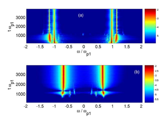
Fig. 16: The ESW spectrum for a beam speed of $v_{b}=0.9c$: (a) shows the frequency power spectrum of $k_{c}=k_{u}$ and (b) shows the frequency power spectrum of $k_{c}=k_{u}/2$ as a function of time. The colour scale shows $\log_{10}W_{2}(\omega,t,k_{c})$. The ESW driven by beam 1 with $v_{b}>0$ corresponds to the wave with $\omega=\omega_{p,1}$ in (b).

For both beam speeds $v_{b}=0.8c$ and $v_{b}=0.9c$ the sideband modes appear to have a superluminal phase speed and they can therefore not trap electrons. No secondary BGK modes should develop for these beam speeds. This is confirmed by Fig. 17 where we show the phase space distribution of the electrons for $v_{b}=0.9c$ at the simulation’s end. The phase space distribution at high momenta shows no evidence of a BGK mode despite the strong sideband modes in Fig. 16.

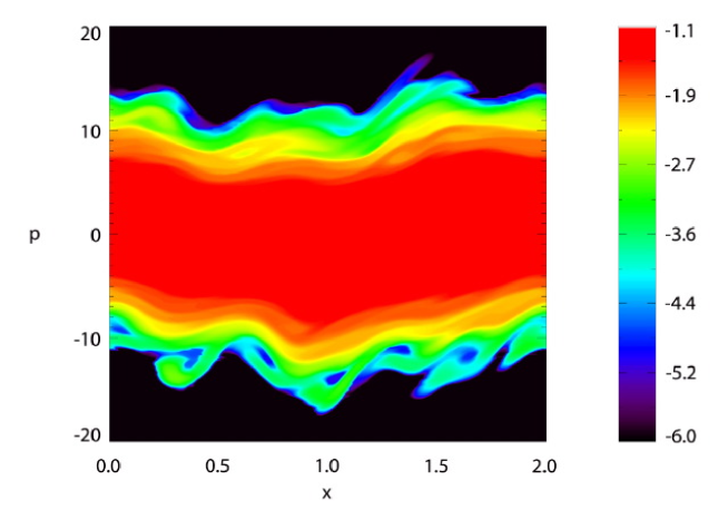
Fig. 17: Contour plot of $\log(f_{e}>10^{-6})$ for $v_{b}=0.9c$ at the time $t=4000$: No well-defined BGK mode is visible in the electron distribution since the sideband unstable modes have a superluminal phase speed.

In contrast to the PIC simulations in Dieckmann et al. ([2004a]) the Vlasov simulation code shows the growth of sideband modes and what appears to be waves resulting from a parametric instability. These secondary waves grow to a large amplitude at which they can nonlinearly interact with the electrons. For the beam speeds up to $v_{b}=0.4c$ the waves generated by the parametric interaction have been strongest. Here the turbulent wave fields interact with the waves with $\omega_{p,1}$ to produce a wave with a higher frequency. In contrast to plasma beat wave accelerators, which have recently been reviewed by Bingham, Mendonca & Shukla ([2004]), for which two high-frequency electromagnetic waves beat to yield a low frequency ESW that can accelerate the electrons, our parametric coupling couples low frequency ESWs to an ESW with a higher frequency. Its larger phase speed can accelerate the trapped electrons to higher peak speeds. We may thus call it the “inverse plasma beat wave accelerator”. For a beam speed of $v_{b}=0.6c$ the turbulent wave fields do not noticably interact with $\omega_{p,1}$. Instead a sideband unstable mode with $k=k_{u}$ develops, i.e. at the largest allowed wave number for nonrelativistic BGK modes (Krasovsky [1994]). This mode has for $v_{b}\leq 0.6c$ a phase speed below $c$ and the electron phase space distribution shows a fast BGK mode driven by it. For even higher $v_{b}$ the probably superluminal phase speed of the sideband modes suppresses their interaction with the electrons.

The complex spectrum of secondary waves and their nonlinear interactions with the electrons, which has not been observed clearly by Dieckmann et al. ([2004a]), suggests a stronger dependence of the electron heating on $v_{b}$ than for the simulations by Dieckmann et al. ([2004a]). There the momentum distributions could be matched if one were to scale the momentum axis to $v_{b}\gamma(v_{b})$. We thus do the same here and we integrate the electron phase space distribution over $x$. The result is shown in Fig. 18.

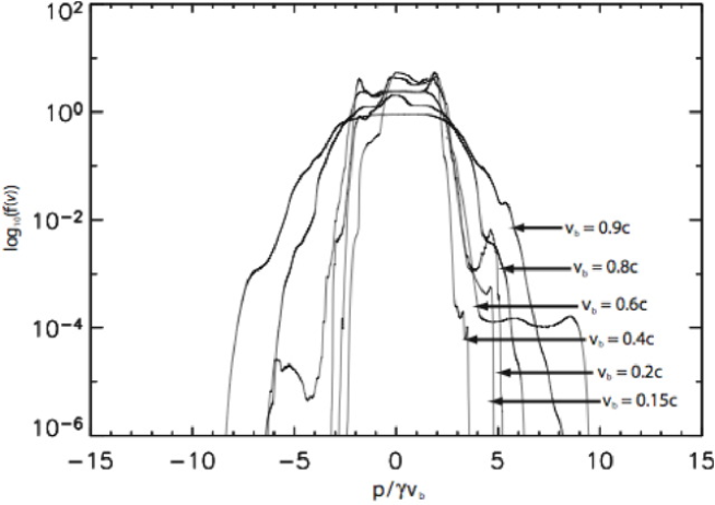
Fig. 18: The electron momentum distributions at the simulation’s end times:

We find that the final momentum distributions in the chosen normalization of the p-axis agree well up to $v_{b}=0.6c$ and for densities larger than $10^{-2}$. Here the Vlasov code results are similar to the equivalent PIC simulations in Dieckmann et al. ([2004a]). We find, however, significant differences at lower densities, which are not well-represented by the PIC code, and at the corresponding higher momenta. The parametric instabilites and the sideband instabilities have further accelerated electrons beyond the peak momenta measured in Dieckmann et al. ([2004a]). This is particularly pronounced for the beam speed $v_{b}=0.6$ in which we find an electron density plateau extending to a value of +10 for the normalised momentum, i. e. twice as high as the corresponding value at negative momenta. For these beam speeds the secondary waves have been most efficient as electron accelerators. A further increase of $v_{b}$ beyond 0.6c yields broadening momentum distributions. The peak momentum in units of $m_{e}c$ is, for positive momenta comparable for $v_{b}=0.6c$ and for $v_{b}=0.8c$. The peak momentum for $v_{b}=0.9c$ is about twice as high as for $v_{b}=0.6c$.

The peak relativistic kinetic energies $K=mc^{2}e^{-1}(\gamma-1)$ in eV the electrons reach are $K(v_{b}=0.15c)=1.3\times 10^{5}$ eV, $K(v_{b}=0.2c)=2.2\times 10^{5}$ eV, $K(v_{b}=0.4c)=5\times 10^{5}$ eV, $K(v_{b}=0.6c)=3.2\times 10^{6}$ eV, $K(v_{b}=0.8c)=3.6\times 10^{6}$ eV and $K(v_{b}=0.9c)=8\times 10^{6}$ eV. Note that all these peak electron energies are comparable or above the threshold energy of $10^{5}$ eV: the injection energy for Fermi acceleration at perpendicular shocks, given by Treumann & Terasawa ([2001]).

fnum@section4 Discussion

The observation of the emission of highly energetic cosmic ray particles by SNRs suggests the acceleration of particles from the thermal pool of the ISM plasma to highly relativistic energies by such objects. The acceleration site is apparently linked to the shock that develops as the supernova blast shell encounters the ambient plasma (Lazendic [2004]). Such shocks are believed to accelerate electrons and ions to highly relativistic energies by means of Fermi acceleration (Fermi [1949]; Fermi [1954]). The Fermi acceleration of electrons is most efficient if the shock is quasi-perpendicular (Galeev [1984]). For such shocks, however, Fermi acceleration works only if we find a relativistically hot electron population prior to the shock encounter, since slow electrons could not repeatedly cross the shock and pick up energy. Since the plasma, into which the SNR shock expands, has a thermal speed comparable to that of the ISM or the stellar wind of the progenitor star with temperatures of up to a few eV, if we take the solar wind as reference, no mildly relativistic electrons may exist. A mechanism is thus required that accelerates electrons up to speeds at which their Larmor radius exceeds the shock thickness. As Galeev ([1984]) proposed, electrons could be pre-accelerated from the initial thermal pool to mildly relativistic energies by their interaction with strong ESWs in the foreshock region which, in turn, are driven by shock-reflected beams of ions.

We have examined in this work the growth, saturation and collapse of ESWs in a system dominated by the presence of two counter-propagating proton beams. The currents of both beams cancel, allowing the introduction of periodic boundary conditions. These initial conditions can be motivated as follows: The upstream protons, that have initially been reflected by the shock, are rotated by the global magnetic field oriented perpendicularly to the shock normal and return as a second counter propagating proton beam, with a slightly increased temperature. The system modelled in this work represents a small region ahead of a SNR shock. Here the magnetic field has been neglected in order to focus on the ESWs and nonlinear BGK modes. While this does not describe a complete model for the foreshock dynamics of high Mach number shocks, it is applicable to parts of the foreshock of perpendicular shocks where local variations magnetic field cause it to vanish, or become beam-aligned. These variations may, for example, be due to the presence of turbulent magnetic field structures in the foreshock of SNR shocks (Jun & Jones [1999]; Lazendic et al. [2004]).

The system is unstable to the relativistic Buneman instability (Thode & Sudan [1973]) which saturates via the trapping of electrons to form BGK modes (Rosenzweig [1988]). These trapped particle distributions are themselves unstable to the sideband instability and collapse after a period of stability.

Since our model assumes that the particle trajectories are not affected by the local magnetic field and because we do not consider here electromagnetic waves or waves in magnetised plasma, we are able to utilise a relativistic, electrostatic Vlasov code. Previous work, for example (Thode & Sudan [1973]; Dieckmann et al. [2000]; Dieckmann et al. [2004b]; Shimada & Hoshino [2004]) has made extensive use of PIC codes for this problem and in particular Dieckmann et al. ([2004b]) have compared Vlasov and PIC codes in certain conditions. We benefit from the Eulerian Vlasov code’s ability to resolve electron and ion phase space accurately, irrespective of the local particle density. This allows us to identify a secondary acceleration mechanism which may not be immediately apparent otherwise. Overall the results of this work are in agreement with previous studies (Dieckmann et al. [2000]; Dieckmann et al. [2004b]) showing the lifetimes of the BGK modes to be dependent on the initial beam velocity. As $v_{b}$ is increased, we observe a reduced ESW stability up to $v_{b}=0.8c$ but with a significantly increased stability at the highest beam speed.

At low beam velocities ($v_{b}=0.15c,0.2c,0.4c,0.6c$) we observe long wavelength, high phase-velocity modes. These are able to trap electrons, producing a population with kinetic energies above the injection energy for Fermi acceleration, even at non-relativistic beam, and thus shock, velocities. We believe these secondary (that is to say, not associated with the initial ESW saturation) trapped distributions to be the result of trapping in ESWs produced by parametric coupling between low frequency oscillations and plasma waves at $\omega_{p,1}$. Above $v_{b}=0.6c$ the ESWs produced by this coupling have super-luminal phase velocities and are unable to trap electrons. Hence we do not observe such BGK modes in the case of $v_{b}=0.8c,$ or $0.9c$. Our simulation box, at $4\pi/k_{u}$ in length, can only accommodate one wavemode with wavenumber below that of the most unstable mode and this may have an influence on the appearance of this secondary acceleration.

Future work has to examine how these parametric instabilities depend on a magnetic field and on the introduction of a second spatial dimension. We will need to consider significantly larger simulation boxes, capable of resolving a broader spectrum below $k_{u}$. It may be the case that the availability of modes with $k<k_{u}$ will result in the partition of ESW energy across a greater region of the spectrum, perhaps inhibiting the trapping of electrons at high velocity. However, it may be the case that our observed coupling and resultant electron trapping is the first step of a cascade, capable of accelerating electrons to high energies for relatively modest shock velocities. This is since, even for $v_{b}$ as low as 0.15c or corresponding shock speeds of $7.5\times 10^{-2}c$ which can be reached by the fastest SNR main shocks (Kulkarni et al. [1998]), electrons can reach energies of $10^{5}$ eV. According to Treumann & Terasawa ([2001]), this may increase the electron gyroradius beyond the shock thickness by which they can repeatedly cross the shock front. These repeated shock crossings allow the electrons to undergo Fermi acceleration to highly relativistic speeds. Even higher energies could be achieved if we were to get shock precursors that outran the main shock as has been observed for the supernova SN1998bw (Kulkarni et al. [1998]). The numerical simulations in this work thus present strong evidence for the ability of ESWs and processes driven by electrostatic turbulence to accelerate electrons beyond the threshold energy at which they can undergo Fermi acceleration as it has previously been proposed, for example by Galeev ([1984]).

fnum@section5 Acknowledgements

This work was supported in part by: the European Commission through the Grant No. HPRN-CT-2001-00314; the Engineering and Physical Sciences Research Council (EPSRC); the German Research Foundation (DFG); and the United Kingdom Atomic Energy Authority (UKAEA). The authors thank the Centre for Scientific Computing (CSC) at the University of Warwick, with support from Science Research Investment Fund grant (grant code TBA), for the provision of computer time. N J Sircombe would like to thank Padma Shukla and the rest of the Institut für Theoretische Physik IV at the Ruhr-Universität Bochum for their kind hospitality during his stay.

References

- [2004] Aharonian, F. A. et al. 2004, Nature, 432, 75
- [2002] Arber, T. D., & Vann, R. G. L. 2002, J. Comput. Phys., 180, 339
- [1957] Bernstein, I. B., Greene, J. M., & Kruskal, M. D. 1957, Phys. Rev., 108, 546
- [1978a] Bell, A. R. 1978a, MNRAS, 182, 147
- [1978b] Bell, A. R. 1978b, MNRAS, 182, 443
- [2004] Bingham, R., Mendonca, J. T., & Shukla, P. K. 2004, Plasma Phys. Control. F., 46, R1
- [2000] Brunetti, M., Califano, F., & Pegoraro F. 2000, Phys. Rev. E, 62, 4109
- [1978] Blandford, R. D. & Ostriker, J. P. 1978, ApJ, 221, L29
- [1958] Buneman, O. 1958, Phys. Rev. Lett., 1, 8
- [1976] Cheng, C. Z., & Knorr, G. 1976, J. Comput. Phys, 22, 330
- [1984] Colella, P., & Woodward, P. R. 1984, J. Comput. Phys, 54, 174
- [2004a] Dieckmann, M. E., Eliasson, B., & Shukla, P. K. 2004a, Phys. Plasmas, 11, 1394
- [2004b] Dieckmann, M. E., Eliasson, B., Stathopoulos A., & Ynnerman A. 2004b, Phys. Rev. Lett., 92, 065006
- [2000] Dieckmann, M. E., Ljung, P., Ynnerman, A., & McClements K. G. 2000, Phys. Plasmas, 7, 5171
- [2002] Dieckmann, M. E., Ljung, P., Ynnerman, A., & McClements, K. G. 2002, IEEE Trans. Plasma Sci., 30, 20
- [2004c] Dieckmann, M. E., Ynnerman, A., Chapman, S. C., Rowlands, G. & Andersson, N. 2004c, Phys. Scr., 69, 456
- [2005] Eastwood, J. P., Lucek, E. A., Mazelle, C., Meziane, K., Narita, Y., Picket, J. & Treumann, R. A. 2005, Space Sci. Rev., 118, 41
- [1991] Eastwood, J. W. 1991, Comput. Phys. Comm., 64, 252
- [2002] Eliasson, B. 2002, J. Comput. Phys., 181, 98
- [2005] Eliasson, B., Dieckmann, M. E., & Shukla, P. K. 2005, New J. Phys., 7, 136
- [1982] Escande, D. F. 1982, Phys. Scripta, T2, 126
- [1949] Fermi, E. 1949, Phys. Rev., 75, 1169
- [1954] Fermi, E. 1954, ApJ, 119, 1
- [1984] Galeev, A. A. 1984, Sov. Phys. J. Exp. Theor. Phys., 59, 965
- [1999] Jun, B. I., & Jones, T. W. 1999, ApJ,, 511, 774
- [1983] Katsouleas, T., & Dawson, J. M. 1983, Phys. Rev. Lett., 51, 392
- [1994] Krasovsky, V. L. 1994, Phys. Scripta, 49, 489
- [1969] Kruer, W. L., Dawson, J. M., & Sudan, R. N. 1969, Phys. Rev. Lett., 23, 838
- [1998] Kulkarni, S. R., Frail, D. A., Wieringa M. H., Ekers, R. D., Sadler E. M., Wark, R. M., Higdon, J. L., Phinney, E. S., & Bloom J. S. 1998, Nature, 395, 663
- [2005] Kuramitsu, Y., Krasnoselskikh, V. 2005, Phys. Rev. Lett., 94, 031102
- [2004] Lazendic, J. S., Slane, P. O., Gaensler, B. M., Reynolds, S. P., Plucinsky, P. P., & Hughes, J. P. 2004, ApJ, 602, 271
- [1992] Lembege, B. & Savoini P. 1992, Phys. Fluids B, 4, 3533
- [2004] Lembege, B., Giacalone, J., Scholer, M., Hada, T., Hoshino, M., Krasnoselskikh, V., Kucharek, H., Savoini, P., & Terasawa, T. 2004, Space Sci. Rev., 110, 161
- [1971] Lovelace, R. V. & Sudan, R. N. 1971, Phys. Rev. Lett., 27, 1256
- [1997] Manfredi, G. 1997, Phys. Rev. Lett., 79, 2815
- [1997] McClements, K. G., Dendy, R. O., Bingham, R., Kirk, J. G., & Drury, L. O. 1997, MNRAS, 291, 241
- [2001] McClements, K. G., Dieckmann, M. E., Ynnerman, A., Chapman, S. C., & Dendy, R. O. 2001, Phys. Rev. Lett., 87, 255002
- [1998] Mohanty, J. N. & Naik, A. 1998, Phys. Plasmas, 5, 915
- [2000] Nagano, M. & Watson, A. A. 2000, Rev. Mod. Phys., 72, 689
- [2001] Reynolds, S. P. 2001, Space Sci. Rev., 99, 177
- [1988] Rosenzweig, J. B. 1988, Phys. Rev. A, 38, 3634
- [1996] Schamel, H. & Korn, J. 1996, Phys. Scripta T63, 63
- [1983] Sckopke, N., Paschmann, G., Bame, S. J., Gosling, J. T. & Russel, C. T. 1983, J. Geophys. Res., 88, 6121
- [2001] Ucer, D., & Shapiro, V. D. 2001, Phys. Rev. Lett., 87, 075001
- [2005] Sircombe, N. J., Arber, T. D., & Dendy, R. O. 2005, Phys. Plasmas, 12, 012303
- [2002] Schmitz, H., Chapman, S. C., & Dendy, R. O. 2002, ApJ,, 579, 327
- [2003] Shapiro, V. D., & Ucer, D. 2003, Planet. Space Sci. 51, 665
- [2000] Shimada, N., & Hoshino, M. 2000, ApJ,, 543, L67
- [2003] Shimada, N., & Hoshino M. 2003, Phys. Plasmas, 10, 1113
- [2004] Shimada, N., & Hoshino M. 2004, Phys. Plasmas, 11, 1840
- [1973] Thode, L. E., & Sudan, R. N. 1973, Phys. Rev. Lett., 30, 732
- [2001] Treumann, R. A., & Terasawa, T. 2001, Space Sci. Rev., 99, 135
- [1989] Tsunoda, S. I., & Malmberg, J. H. 1989, Phys. Fluids B, 1, 1958
- [1988] Völk, H. J., Zank, L. A. & G. P. Zank 1988, A& A, 198, 274
- [1990] Zank, P., Axford, W. I. & McKenzie, J. F. 1990, A& A, 233, 275