Van Kampen’s expansion approach in an opinion formation model

Abstract

We analyze a simple opinion formation model consisting of two parties, $A$ and $B$, and a group $I$, of undecided agents. We assume that the supporters of parties $A$ and $B$ do not interact among them, but only interact through the group $I$, and that there is a nonzero probability of a spontaneous change of opinion ($A\leftrightarrows I$, $B\leftrightarrows I$). From the master equation, and via van Kampen’s $\Omega$-expansion approach, we have obtained the “macroscopic” evolution equation, as well as the Fokker-Planck equation governing the fluctuations around the deterministic behavior. Within the same approach, we have also obtained information about the typical relaxation behavior of small perturbations.

I Introduction

The last few years have witnessed a growing interest among theoretical physicists in complex phenomena in fields departing from the classical mainstream of physics research. In particular, the application of statistical physics methods to social phenomena has been discussed in several reviews weidlich1 ; weidlich2 ; stauffer00 ; stauffer00p ; Galam000 . Among these sociological problems, one that has attracted much attention was the building (or the lack) of consensus. There are many different models that simulate and analyze the dynamics of such processes in opinion formation, cultural dynamics, etc Galam000 ; Gal00 ; complex1 ; heg01 ; sznajd01 ; sznajd02 ; stauffer1 ; stauffer2 ; stauffer3 ; Castellano ; Klemm1 ; krapi01 ; Mobilia1 ; nos ; schneider1 ; JRI . Even though in general the models studied in those works are simple ones, most of the results have been obtained via simulations. However, it is extremely relevant to have some form of analytical insight.

In this work we analyze a simple opinion formation model, analogous to the one studied in redner3 consisting of two parties, $A$ and $B$, and an “intermediate” group $I$, that we call undecided agents. As in redner3 , we assume that the supporters of parties $A$ and $B$ do not interact among them, but only through their interaction with the group $I$, convincing one of its members through a Sznajd-like rule similarly to what was discussed in sznajd02 , that is within a mean-field treatment. However, we don’t consider that members of $I$ can convince those of $A$ or $B$, but instead we assume that there is a nonzero probability of a spontaneous change of opinion from $I$ to the other two parties and viceversa: $I\leftrightarrows A$, and $\,I\leftrightarrows B$. We will see that this probability of spontaneous change of opinion (implying the existence of a social temperature babinec ; weidlich2 ; last ) inhibits the possibility of reaching a consensus. Instead of consensus, we find that each party has some statistical density of supporters, and there is also a statistical stationary number of undecided ($I$) agents.

Our aim is to write a master equation for this toy model, and study its behavior via van Kampen’s $\Omega$-expansion approach vKamp . After determining if, in this case, the conditions for the validity of using such an approach are fulfilled, and exploiting it, we could obtain the macroscopic evolution equations for the density of supporters of $A$ and $B$ parties, as well as the Fokker-Planck equation governing the fluctuations around such deterministic or macroscopic behavior. The same approach also offers information about the typical relaxation behavior of small perturbations around the stationary macroscopic solutions.

The outline of the paper is the following. In the next Section we present the model, and apply van Kampen’s $\Omega$ expansion approach in order to obtain the macroscopic equation and the Fokker-Planck equation governing the fluctuations around the macroscopic behavior. In Section 3 we analyze the behavior of the fluctuations through the study of their mean values and correlations, and discuss the relaxation time of small perturbations. In Section 4 we present some typical results and finally, in Section 5, some general conclusions are summarized.

II The model and the approach

II.1 Description of the model

We consider a system composed of three different groups of agents
$\triangleright$ supporters of the $A$ party, indicated by $N_{A}$,
$\triangleright$ supporters of the $B$ party, indicated by $N_{B}$,
$\triangleright$ undecided ones, indicated by $N_{I}$.
The interactions we are going to consider are only between $A$ and $I$, and $B$ and $I$. That means that we do not include direct interactions among $A$ and $B$. The different contributions that we include are
$\bullet$ spontaneous transitions $A\to I$, occurring with a rate $\alpha_{1}\,N_{A}$;
$\bullet$ spontaneous transitions $I\to A$, occurring with a rate $\alpha_{2}\,N_{I}$;
$\bullet$ spontaneous transitions $B\to I$, occurring with a rate $\alpha_{3}\,N_{B}$;
$\bullet$ spontaneous transitions $I\to B$, occurring with a rate $\alpha_{4}\,N_{I}$;
$\bullet$ convincing rule $A+I\to 2\,A$, occurring with rate $\frac{\beta_{1}}{\Omega}N_{A}N_{I}$;
$\bullet$ convincing rule $B+I\to 2\,B$, occurring with rate $\frac{\beta_{2}}{\Omega}N_{B}N_{I}$.
As indicated above, here $N_{i}$ is the number of agents supporting the party or group “$i$” (with $i=A,B,I$). We have the constraint $N_{A}+N_{B}+N_{I}=N$, where $N$ is the total number of agents. Such a constraint implies that, for fixed $N$, there are only two independent variables $N_{A}$ and $N_{B}$. By using this constraint, the rates indicated above associated to processes involving $N_{I}$, could be written replacing $N_{I}=(N-N_{A}-N_{B}).$

With the above indicated interactions and rates, the master equation for the probability $P(N_{A},N_{B},t)$ of having populations $N_{A}$ and $N_{B}$ at time $t$ (due we have had populations $N_{A}^{o}$ and $N_{B}^{o}$ at an initial time $t_{o}(<t)$), may be written as

$$\frac{\partial}{\partial\,t}P(N_{A},N_{B},t)= \alpha_{1}(N_{A}+1)P(N_{A}+1,N_{B},t)+\alpha_{3}(N_{B}+1)P(N_{A},N_{B}+1,t)$$ (1)

$$+ \alpha_{2}(N-N_{A}-N_{B}+1)P(N_{A}-1,N_{B},t)$$

$$+ \alpha_{4}(N-N_{A}-N_{B}+1)P(N_{A},N_{B}-1,t)$$

$$+ \frac{\beta_{1}}{\Omega}(N_{A}-1)(N-N_{A}-N_{B}+1)P(N_{A}-1,N_{B},t)$$

$$+ \frac{\beta_{2}}{\Omega}(N_{B}-1)(N-N_{A}-N_{B}+1)P(N_{A},N_{B}-1,t)$$

$$- \Bigl{[}\alpha_{1}N_{A}+\alpha_{3}N_{B}+\alpha_{2}(N-N_{A}-N_{B})\Bigr{.}$$

$$\,\,\,\,\,\,\,\,\,\,\,\,\,\,\,+\Bigl{.}\alpha_{4}(N-N_{A}-N_{B}+1)\Bigr{]}P(N_{A},N_{B},t).$$

This is the model master equation to which we will apply van Kampen’s approach vKamp .

II.2 Van Kampen’s expansion

In order to apply van Kampen’s approach, as discussed in vKamp , we identify the large parameter $\Omega$ with $N$ (assuming $N\gg 1$); and define the following separation of the $N_{i}$’s into a macroscopic part of size $\Omega$, and a fluctuational part of size $\Omega^{\frac{1}{2}}$,

$$N_{A} = \Omega\Psi_{A}(t)+\Omega^{\frac{1}{2}}\xi_{A}(t),$$

$$N_{B} = \Omega\Psi_{B}(t)+\Omega^{\frac{1}{2}}\xi_{B}(t),$$ (2)

and define the density $\rho=\frac{N}{\Omega}$ (in our case $\rho=1$). We also define the “step operators”

$$\mathbb{E}_{i}^{1}f(N_{i}) = f(N_{i}+1),$$

$$\mathbb{E}_{i}^{-1}f(N_{i}) = f(N_{i}-1),$$

with $f(N_{i})$ an arbitrary function. Using the forms indicated in Eqs. (II.2), in the limit of $\Omega\gg 1$, the step operators adopt the differential form vKamp

$$\mathbb{E}_{i}^{\pm 1}=1\pm\left(\frac{1}{\Omega}\right)^{\frac{1}{2}}\frac{\partial}{\partial\,\xi_{i}}+\frac{1}{2}\left(\frac{1}{\Omega}\right)\frac{\partial^{2}}{\partial\,\xi_{i}^{2}}\pm\ldots,$$ (3)

with $i=A,B$. Transforming from the old variables $(N_{A},N_{B})$ to the new ones $(\xi_{A},\xi_{B})$, we have the relations

$$P(N_{A},N_{B},t) \rightarrow \Pi(\xi_{A},\xi_{B},t),$$ (4)

$$\Omega^{\frac{1}{2}}\frac{\partial}{\partial\,N_{i}}P(N_{A},N_{B},t) = \frac{\partial}{\partial\,\xi_{i}}\Pi(\xi_{A},\xi_{B},t).$$ (5)

Putting everything together, and considering contributions up to order $\Omega^{\frac{1}{2}}$, yields the following two coupled differential equations for the macroscopic behavior

$$\frac{d}{dt}\Psi_{A}(t)=-\alpha_{1}\Psi_{A}+\Bigl{[}\alpha_{2}+\beta_{1}\Psi_{A}\Bigr{]}\Bigl{(}\rho-\Psi_{A}-\Psi_{B}\Bigr{)},$$ (6)

$$\frac{d}{dt}\Psi_{B}(t)=-\alpha_{3}\Psi_{B}+\Bigl{[}\alpha_{4}+\beta_{2}\Psi_{B}\Bigr{]}\Bigl{(}\rho-\Psi_{A}-\Psi_{B}\Bigr{)}.$$ (7)

It can be proved that the last set of equations has a unique (physically sound) stationary solution, i.e. a unique attractor

$$\Psi_{A}(t\to\infty) = \Psi_{A}^{st}$$

$$\Psi_{B}(t\to\infty) = \Psi_{B}^{st}.$$

This is the main condition to validate the application of van Kampen’s $\Omega$-expansion approach vKamp .

The following order, that is $\Omega^{0}$, yields the Fokker-Planck equation (FPE) governing the fluctuations around the macroscopic behavior. It is given by

$$\frac{\partial}{\partial\,t}\Pi(\xi_{A},\xi_{B},t)= \frac{\partial}{\partial\xi_{A}}\Bigl{[}\left(\alpha_{1}\xi_{A}+(\alpha_{2}+\beta_{1}\Psi_{A})(\xi_{A}+\xi_{B})-\beta_{1}\xi_{A}(\rho-\Psi_{A}-\Psi_{B})\right)\Pi(\xi_{A},\xi_{B},t)\Bigr{]}$$ (8)

$$+ \frac{\partial}{\partial\xi_{B}}\Bigl{[}\left(\alpha_{3}\xi_{B}+(\alpha_{4}+\beta_{2}\Psi_{B})(\xi_{A}+\xi_{B})-\beta_{2}\xi_{B}(\rho-\Psi_{A}-\Psi_{B})\right)\Pi(\xi_{A},\xi_{B},t)\Bigr{]}$$

$$+ \frac{1}{2}\Bigl{[}\alpha_{1}\Psi_{A}+(\alpha_{2}+\beta_{1}\Psi_{A})(\rho-\Psi_{A}-\Psi_{B})\Bigr{]}\frac{\partial^{2}}{\partial\xi_{A}^{2}}\Pi(\xi_{A},\xi_{B},t)$$

$$+ \frac{1}{2}\Bigl{[}\alpha_{3}\Psi_{B}+(\alpha_{4}+\beta_{2}\Psi_{B})(\rho-\Psi_{A}-\Psi_{B})\Bigr{]}\frac{\partial^{2}}{\partial\xi_{B}^{2}}\Pi(\xi_{A},\xi_{B},t).$$

As is well known for this approach vKamp , the solution of this FPE will have a Gaussian form determined by the first and second moments of the fluctuations. Hence, in the next section we analyze the equations governing those quantities.

III Behavior of fluctuations

From the FPE indicated above (Eq. (8)), it is possible to obtain equations for the mean value of the fluctuations as well as for the correlations of those fluctuations. For the fluctuations, $\langle\xi_{A}(t)\rangle=\eta_{A}$ and $\langle\xi_{B}(t)\rangle=\eta_{B}$, we have

$$\frac{d}{dt}\eta_{A}(t) = -\Bigl{[}\alpha_{1}+\alpha_{2}+\beta_{1}(2\Psi_{A}+\Psi_{B})-\beta_{1}\rho\Bigr{]}\eta_{A}-(\alpha_{2}+\beta_{1}\Psi_{A})\eta_{B}$$ (9)

$$\frac{d}{dt}\eta_{B}(t) = -\Bigl{[}\alpha_{3}+\alpha_{4}+\beta_{2}(\Psi_{A}+2\Psi_{B})-\beta_{2}\rho\Bigr{]}\eta_{B}-(\alpha_{4}+\beta_{2}\Psi_{B})\eta_{A}.$$ (10)

Calling $\sigma_{A}=\langle\xi_{A}(t)^{2}\rangle$, $\sigma_{B}=\langle\xi_{B}(t)^{2}\rangle$, and $\sigma_{AB}=\langle\xi_{A}(t)\xi_{B}(t)\rangle$, we obtain for the correlation of fluctuations

$$\frac{d}{dt}\sigma_{A}(t) = -2\alpha_{1}\sigma_{A}-2[\alpha_{2}+\beta_{1}\Psi_{A}][\sigma_{A}+\sigma_{AB}]+2\beta_{1}\sigma_{A}[\rho-\Psi_{A}-\Psi_{B}]$$ (11)

$$\,\,\,\,\,\,\,\,\,\,\,\,\,\,\,\,+[\alpha_{1}\Psi_{A}+(\alpha_{2}+\beta_{1}\Psi_{A})(\rho-\Psi_{A}-\Psi_{B})],$$

$$\frac{d}{dt}\sigma_{B}(t) = -2\alpha_{3}\sigma_{B}-2[\alpha_{4}+\beta_{2}\Psi_{B}][\sigma_{AB}+\sigma_{B}]+2\beta_{2}\sigma_{B}[\rho-\Psi_{A}-\Psi_{B}]$$ (12)

$$\,\,\,\,\,\,\,\,\,\,\,\,\,\,\,\,+[\alpha_{3}\Psi_{B}+(\alpha_{4}+\beta_{2}\Psi_{B})(\rho-\Psi_{A}-\Psi_{B})],$$

$$\frac{d}{dt}\sigma_{AB}(t) = -[\alpha_{1}+\alpha_{3}]\sigma_{AB}-[\alpha_{2}+\beta_{1}\Psi_{A}][\sigma_{AB}+\sigma_{B}]$$ (13)

$$\,\,\,\,\,\,\,\,\,\,\,\,\,\,\,\,-[\alpha_{4}+\beta_{2}\Psi_{B}][\sigma_{A}+\sigma_{AB}]+[\rho-\Psi_{A}-\Psi_{B}][\beta_{1}+\beta_{2}]\sigma_{AB}.$$

III.1 Reference state: symmetric case

Here we particularize the above indicated equations to the symmetrical case, i.e. the case when $\Psi_{A}^{st}=\Psi_{B}^{st}$. Hence, we adopt

$$\alpha_{1}=\alpha_{3}=\alpha,\,\,\,\,\,\alpha_{2}=\alpha_{4}=\alpha^{\prime},$$

and

$$\beta_{1}=\beta_{2}=\beta.$$

In such a case, the macroscopic equations (6) and (7) take the form

$$\frac{d}{dt}\Psi_{A}(t) = -[\alpha+\alpha^{\prime}-\beta]\Psi_{A}-\beta\Psi_{A}^{2}-\beta\Psi_{A}\Psi_{B}-\alpha^{\prime}\Psi_{B}+\alpha^{\prime}$$ (14)

$$\frac{d}{dt}\Psi_{B}(t) = -[\alpha+\alpha^{\prime}-\beta]\Psi_{B}-\beta\Psi_{B}^{2}-\beta\Psi_{A}\Psi_{B}-\alpha^{\prime}\Psi_{A}+\alpha^{\prime}.$$ (15)

In order to make more explicit the solution of these equations, we work with the auxiliary variables $\Sigma=\Psi_{A}+\Psi_{B}$ and $\Delta=\Psi_{A}-\Psi_{B}$, and use $\rho=1$. Hence, the last equations transform now into

$$\frac{d}{dt}\Sigma(t) = -\Bigl{[}\alpha+2\alpha^{\prime}-\beta\Bigr{]}\,\Sigma-\beta\Sigma^{2}+2\alpha^{\prime}$$ (16)

$$\frac{d}{dt}\Delta(t) = -\Bigl{[}\alpha-\beta\Bigr{]}\,\Delta-\beta\Delta\Sigma.$$ (17)

In the long time limit, $t\to\infty$, we found on one hand

$$\Delta^{st}=0,$$

implying $\Psi_{A}^{st}=\Psi_{B}^{st}$, while on the other hand

$$0=\beta\,\Sigma^{2}+\Bigl{[}\alpha+2\alpha^{\prime}-\beta\Bigr{]}\,\Sigma-2\alpha^{\prime}.$$

This polynomial has two roots, but only one is physically sound, namely

$$\Sigma^{st}=\frac{\alpha+2\alpha^{\prime}-\beta}{2\beta}\left(-1+\sqrt{1+\frac{8\alpha^{\prime}\beta}{[\alpha+2\alpha^{\prime}-\beta]^{2}}}\right),$$ (18)

yielding $\Psi_{A}^{st}=\Psi_{B}^{st}=\Psi_{o}^{st}=\frac{1}{2}\Sigma^{st}.$

In a similar way, we can also simplify the equations for $\eta_{A}$ and $\eta_{B}$, calling $S(t)=\eta_{A}+\eta_{B}$ and $D(t)=\eta_{A}-\eta_{B}$. The corresponding equations are then rewritten as

$$\frac{d}{dt}S(t) = -\Bigl{[}\alpha+2\alpha^{\prime}+2\beta(\Psi_{A}+\Psi_{B})-\beta\Bigr{]}\,S,$$ (19)

$$\frac{d}{dt}D(t) = -\Bigl{[}\alpha+\beta(\Psi_{A}+\Psi_{B})-\beta\Bigr{]}D-\beta\Bigl{[}\Psi_{a}-\Psi_{B}\Bigr{]}S,,$$ (20)

while for the correlation of the fluctuations we have

$$\frac{d}{dt}\sigma_{A}(t) = -2\alpha\sigma_{A}-2[\alpha^{\prime}+\beta\Psi_{A}][\sigma_{A}+\sigma_{AB}]+2\beta[1-\Psi_{A}-\Psi_{B}]\sigma_{A}$$ (21)

$$\,\,\,\,\,+\left[\alpha\Psi_{A}+(\alpha^{\prime}+\beta\Psi_{A})(1-\Psi_{A}-\Psi_{B})\right],$$

$$\frac{d}{dt}\sigma_{B}(t) = -2\alpha\sigma_{B}-2[\alpha^{\prime}+\beta\Psi_{B}][\sigma_{AB}+\sigma_{B}]+2\beta[1-\Psi_{A}-\Psi_{B}]\sigma_{B}$$ (22)

$$\,\,\,\,\,+\left[\alpha\Psi_{B}+(\alpha^{\prime}+\beta\Psi_{B})(1-\Psi_{A}-\Psi_{B})\right],$$

$$\frac{d}{dt}\sigma_{AB}(t) = -2\alpha\sigma_{AB}-[\alpha^{\prime}+\beta\Psi_{A}][\sigma_{AB}+\sigma_{B}]$$ (23)

$$\,\,\,\,\,-[\alpha^{\prime}+\beta\Psi_{B}][\sigma_{AB}+\sigma_{A}]+2\beta[1-\Psi_{A}-\Psi_{B}]\sigma_{AB}.$$

Equations (19) and (20) show that, in the asymptotic limit, i.e. for $t\to\infty$, both, $S=0$ and $D=0$, implying that $\eta_{A}^{st}=\eta_{B}^{st}=0$. However, also in the general (non symmetric) case we expect to find $\eta_{A}^{st}=\eta_{B}^{st}=0$. In addition, from Eqs. (21), (22) and (23), it is clear that in general we obtain, again for $t\to\infty$, that $\sigma_{i}^{st}\neq 0$ ($i=A,B,AB$).

As we have seen, in the symmetric case we have $\Psi_{A}^{st}=\Psi_{B}^{st}=\Psi_{o}^{st}$, hence it is clear that $\sigma_{A}(t)$ and $\sigma_{B}(t)$ behave in a similar way. And in particular $\sigma_{A}^{st}=\sigma_{B}^{st}=\sigma_{o}^{st}$. In order to analyze the typical time for return to the stationary situation under small perturbations, we assume small perturbations of the form $\sigma_{i}^{st}\approx\sigma_{o}^{st}+\delta\sigma_{i}(t)$ ($i=A,B$) and $\sigma_{AB}^{st}\approx\sigma_{AB,o}^{st}+\delta\sigma_{i}(t),$ and fix $\Psi_{A}^{st}=\Psi_{B}^{st}=\Psi_{o}^{st}.$ We find again that both $\delta\sigma_{A}(t)$ and $\delta\sigma_{B}(t)$ behave in the same way, and this help us to reduce the number of equations for the decay of correlations. Hence, we can put $\delta\sigma_{A}(t)=\delta\sigma_{B}(t)=\delta\sigma_{o}(t).$ The system driving the correlations becomes

$$\frac{d}{dt}\delta\sigma_{o}(t) = -2\Bigl{[}\alpha+\alpha^{\prime}-\beta+3\,\beta\Psi_{o}^{st}\Bigr{]}\delta\sigma_{o}-2\Bigl{[}\alpha^{\prime}+\beta\Psi_{o}^{st}\Bigr{]}\delta\sigma_{AB}$$ (24)

$$\frac{d}{dt}\delta\sigma_{AB}(t) = -2\Bigl{[}\alpha+\alpha^{\prime}-\beta+3\,\beta\Psi_{o}^{st}\Bigr{]}\delta\sigma_{AB}-2\Bigl{[}\alpha^{\prime}+\beta\Psi_{o}^{st}\Bigr{]}\delta\sigma_{o}.$$ (25)

Clearly, $\delta\sigma_{o}^{st}=\delta\sigma_{ab}^{st}\equiv 0.$ After some algebraic steps we obtain

$$\delta\sigma_{o}(t) \simeq \delta\sigma_{o}(0)\,\exp{\Bigl{[}-2[\alpha+2\beta\Psi_{o}^{st}-\beta]\,t\Bigr{]}}$$ (26)

$$\delta\sigma_{AB}(t) \simeq \delta\sigma_{AB}(0)\,\exp{\Bigl{[}-2[\alpha+2\beta\Psi_{o}^{st}-\beta]\,t\Bigr{]}}.$$ (27)

These results indicate that, for the symmetrical case, the typical relaxation time is given by

$$\tau_{relax}=\frac{1}{2}[\alpha+2\beta\Psi_{o}^{st}-\beta]^{-1}.$$ (28)

III.2 Beyond the symmetric case

Let us call $\alpha_{o}$, $\alpha_{o}^{\prime}$ and $\beta_{o}$ to the parameter’s values corresponding to the symmetric case. We consider now the following cases where we vary the parameters

$$\beta_{1}=\beta_{o},\,\,\,\,\,\,\beta_{2}=\beta_{o}+\Delta\beta,$$

$$\alpha_{1}=\alpha_{o},\,\,\,\,\,\,\alpha_{3}=\alpha_{o}+\Delta\alpha,$$

$$\alpha_{2}=\alpha_{o}^{\prime},\,\,\,\,\,\,\alpha_{4}=\alpha_{o}^{\prime}+\Delta\alpha^{\prime}.$$

We will vary only one of these parameters, while keeping the rest fixed. In the following section we present the results (mainly numerical) corresponding to those different cases.

IV Results

As indicated above, the macroscopic equations (Eqs. (6) and (7)) have a unique attractor, indicating that it is adequate to apply van Kampen’s expansion approach. In this section we will present some results corresponding to symmetric and asymmetric situations, that show some typical behavior to be expected from the model and the approximation method. In what follows, al parameters are measured in arbitrary units.

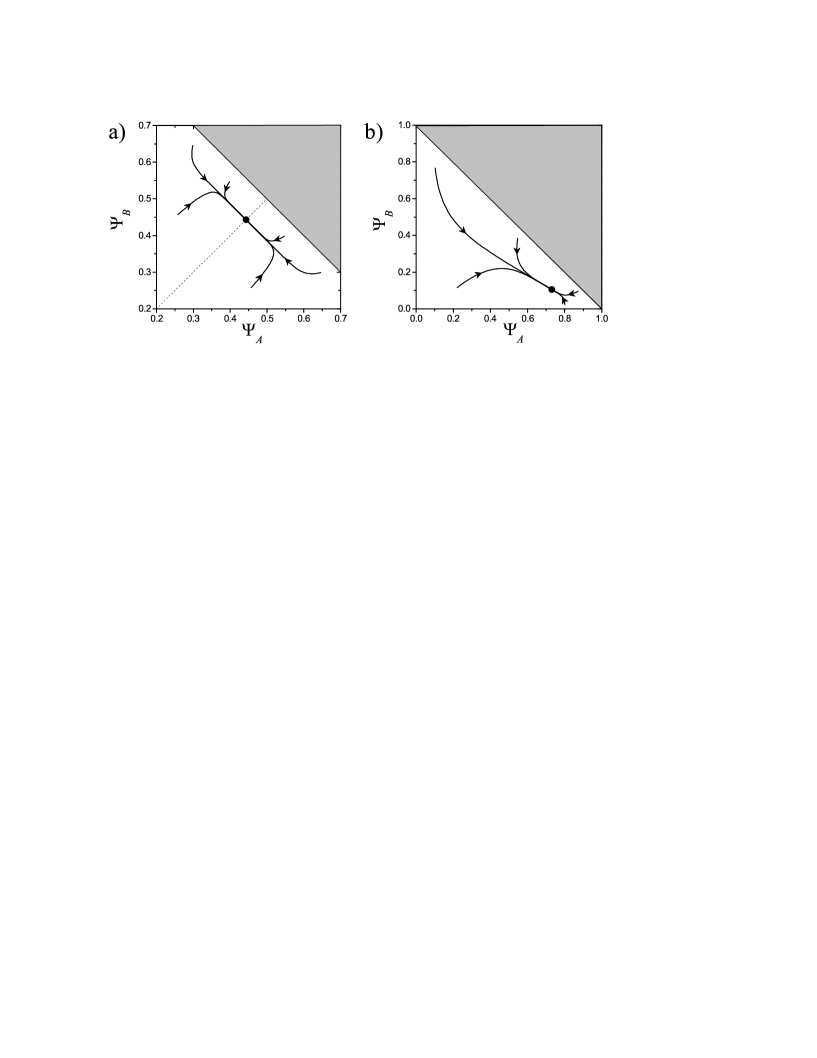
Figure 1: Evolution of the macroscopic solutions (Eqs.(6,7)). Case (a) corresponds to trajectories towards a symmetric solution (i.e. with $\Psi_{A}^{st}=\Psi_{B}^{st}$), with parameters $\alpha_{1}=\alpha_{3}=1$, $\alpha_{2}=\alpha_{4}=3$, and $\beta_{1}=\beta_{2}=2.$ Case (b) corresponds to trajectories towards an asymmetric solution (i.e. with $\Psi_{A}^{st}\neq\Psi_{B}^{st}$), with parameters $\alpha_{1}=1$, $\alpha_{3}=5$, $\alpha_{2}=\alpha_{4}=3$, and $\beta_{1}=\beta_{2}=2.$

In Fig. 1 we show the evolution of $\Psi_{A}(t)$ and $\Psi_{B}(t)$, the macroscopic solutions, indicating some trajectories towards the attractor: (a) for a symmetric, and (b) an asymmetric case. It is worth recalling that $\Psi_{A}$ and $\Psi_{B}$ are the density of supporters of party $A$ and party $B$, respectively. During the evolution towards the attractor, starting from arbitrary initial conditions, we observe the possibility of a marked initial increase of the macroscopic density for one of the parties, follow by a marked reduction, or other situations showing only a decrease of an initial high density. Such cases indicate the need of taking with care the results of surveys and polls during, say, an electoral process. It is possible that an impressive initial increase in the support of a party can be followed for an also impressive decay of such a support.

We remark that, due to the symmetry of the problem, it is equivalent to vary the set of parameters ($\alpha_{3},\alpha_{4},\beta_{2}$) or the set ($\alpha_{1},\alpha_{2},\beta_{1}$). Also worth remarking is That in both panels of Fig 1 the sum of $\Psi_{A}$ and $\Psi_{B}$ is always $<1$, so verifying that there is always a finite fraction of undecided agents.

Figure 2: Dependence of the stationary macroscopic solutions on different system parameters: (a) on $\alpha_{3}$, the rest of parameters are $\alpha_{1}=\alpha_{2}=\alpha_{4}=1$, and $\beta_{1}=\beta_{2}=1.$ (b) on $\alpha_{4}$, the rest of parameters are $\alpha_{1}=\alpha_{2}=\alpha_{3}=1$, and $\beta_{1}=\beta_{2}=1.$ (c) on $\beta_{2}$, the rest of parameters are $\alpha_{1}=\alpha_{2}=\alpha_{3}=\alpha_{4}=1$, and $\beta_{1}=1.$ In all three cases, the continuous line corresponds to $\Psi_{A}^{st}$ while $\Psi_{B}^{st}$ is indicated by the dotted line.

In Fig. 2 we depict the dependence of the stationary macroscopic solutions on different parameters of the system. On Fig. 2(a) the dependence on $\alpha_{3}$ is represented. It is apparent that for $\alpha_{3}<\alpha_{1}$, we have $\Psi_{B}^{st}<\Psi_{A}^{st}$, while for $\alpha_{3}>\alpha_{1}$, we find the inverse situation. Clearly, $\Psi_{B}^{st}=\Psi_{A}^{st}$ when $\alpha_{3}=1(=\alpha_{1})$, as it corresponds to the symmetric case. Similarly, in Figs. 2(b) and 2(c) we see the dependence of the stationary macroscopic solutions on the parameters $\alpha_{4}$ and $\beta_{2}$, respectively. Also in these cases we observe similar behavior as in the previous one, when varying the indicated parameters. The parameters $\alpha_{3}$ or $\alpha_{4}$ (and similarly for $\alpha_{1}$ or $\alpha_{2}$) correspond to spontaneous changes of opinion, and may be related to a kind of social temperature babinec ; weidlich2 ; last . However, also $\beta_{1}$ and $\beta_{2}$ are affected by such a temperature. So, the variation of these parameters in Fig. 2 correspond to changes in the social temperature, changes that could be attributed, in a period of time preceding an election, to increase in the level of discussions as well as the amount of propaganda.

Figure 3: Dependence of the stationary correlation functions $\sigma_{i}$ (with $i=1,2$) corresponding to the projection of $\sigma_{A,B,AB}$ on the principal axes, on different parameters of the system: (a) on $\alpha_{3}$, the other parameters are $\alpha_{1}=\alpha_{2}=\alpha_{3}=1$, and $\beta_{1}=\beta_{2}=1.$ (b) on $\alpha_{4}$, the other parameters are $\alpha_{1}=\alpha_{2}=\alpha_{3}=1$, and $\beta_{1}=\beta_{2}=1.$ (b) on $\beta_{2}$, the other parameters are $\alpha_{1}=\alpha_{2}=\alpha_{3}=\alpha_{4}=1$, and $\beta_{1}=1.$

In Fig. 3 we depict the dependence of the stationary correlation functions for the fluctuations $\sigma_{i}$ (with $i=1,2$, corresponding to the projection of $\sigma_{A,B,AB}$ on the principal axes), on different systems’ parameters. In Fig. 3(a) the dependence on $\alpha_{3}$ is represented, and similarly in Figs. 3(b) and 3(c), the dependence on the parameters $\alpha_{4}$ and $\beta_{2}$, respectively. We observe that, as the parameters are varied (that, in the case of $\alpha_{3}$ and $\alpha_{4}$, and as indicated above, could be associated to a variation of the social temperature) a tendency inversion could arise. This indicates that the dispersion of the probability distribution could change with a variation of the social temperature. This is again a warning for taking with some care the results of surveys and polls previous to an electoral process.

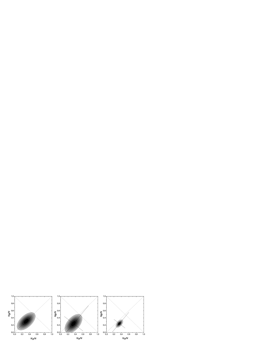
Figure 4: Stationary, Gaussian, probability distribution $\Pi(\xi_{A},\xi_{B})^{st}$ projected on the original $(N_{A},N_{B})$ plane. On the let we have a symmetrical case with $\alpha_{1}=\alpha_{3}=2$, $\alpha_{2}=\alpha_{4}=1$, $\beta_{1}=\beta_{2}=2$, and the population is $N=100$. The central plot shows an asymmetrical case, with $\alpha_{1}=2$ and $\alpha_{3}=2.5$, while $\alpha_{2}=\alpha_{4}=1$, $\beta_{1}=\beta_{2}=2$, and the population is $N=100$. On the right we have the same asymmetrical case as before, but now $N=1000$, showing the dispersion’s reduction of the Gaussian distribution.

Figure 4 shows the stationary (Gaussian) probability distribution (pdf) $\Pi(\xi_{A},\xi_{B})^{st}$ projected on the original $(N_{A},N_{B})$ plane. We show three cases: on the left a symmetrical case, the central one corresponds to an asymmetrical situation with a population of $N=100$, and on the right the same asymmetrical situation but with a population of $N=1000$. This last case clearly shows the influence of the population number in reducing the dispersion (as the population increases). We can use this pdf in order to estimate the probability $p_{i}$ $(i=A,B)$, of winning for one or the other party. It corresponds to the volume of the distribution remaining above, or below, the bisectrix $N_{A}/N=N_{B}/N.$ In the symmetrical case, as is obvious, we obtain $p_{A}=p_{B}=0.5$ (or $50\%$), while in the asymmetrical case we found $p_{B}=0.257$ (or $25.7\%$) and $p_{B}=0.015$ (or $1.5\%$) for $N=100$ and $N=1000$, respectively. These results indicate that, for an asymmetrical situation like the one indicated here, we have a non zero probability that the minority party could, due to a fluctuation during the voting day, win the election. However, in agreement with intuition, as far as $N\gg 1$, and the stationary macroscopic solution departs from the symmetric case, such a probability $p_{i}$ reduces proportionally to $N^{-1}$ comment .

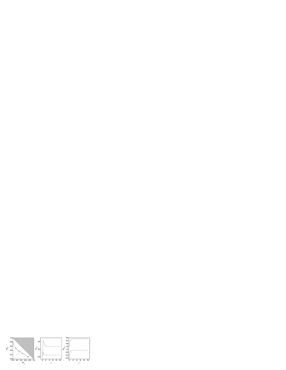
Figure 5: On the left, we have the time evolution of the macroscopic solutions $\Psi_{A}(t)$ and $\Psi_{B}(t)$. The parameter values are $\alpha_{1}=1$, $\alpha_{3}=5$, $\alpha_{2}=\alpha_{4}=3$, $\beta_{1}=\beta_{2}=2$. The stars indicate the position where the maxima that appear in the next panel occurs. Central part, time evolution of the correlation functions $\sigma_{i}$ (with $i=1,2$) corresponding to the projection of $\sigma_{A,B,AB}$ on the principal axes. On the right, the angle between the principal axes and the figure axes. The parameters are $\alpha_{1}=1$, $\alpha_{3}=5$, $\alpha_{2}=\alpha_{4}=3$, and $\beta_{1}=\beta_{2}=2.$

In Fig. 5, on the left, we show a typical result for the time evolution of the macroscopic solution towards an asymmetric stationary case. In the same figure, in the central part we find the associated time evolution of the correlation functions for the fluctuations, $\sigma_{i}$ (with $i=1,2$) corresponding to the projection of $\sigma_{A,B,AB}$ on the principal axes, while on the right we show the evolution of the angle between the principal axes and the figure axes. The temporal reentrance effect that has been observed in other studies exploiting the van Kampen’s approach vKamp ; ich-1 is apparent. This is a new warning, indicating the need to take with some care the results of surveys and polls during an electoral process.

Figure 6: Dependence of the dominant relaxation time on different system parameters. On the left, symmetrical case: continuous line varying $\alpha_{1}=\alpha_{3}$, dotted line varying $\alpha_{2}=\alpha_{4}$, and dashed line varying $\beta_{1}=\beta_{2}$. In order to compare all three, the dotted line was multiplied by 3, while the dashed one by 10. The inset shows, now on the same scale, the crossing of the lines at the point where all the parameters are equal to 1. On the right, asymmetrical case: continuous line varying $\alpha_{1}$, dotted line varying $\alpha_{2}$, and dashed line varying $\beta_{1}$. In all cases, the parameters that remain constant are all $=1$.

In Fig. 6 we depict the dependence of the dominant (or relevant) relaxation time, that is the slowest of the three relaxation times, on different parameters of the system. On the left, we show a symmetrical case where the different lines represent the dependence respect to variation of: $\alpha_{1}=\alpha_{3}$ indicated by a continuous line; $\alpha_{2}=\alpha_{4}$ indicated by dotted line; $\beta_{1}=\beta_{2}$ indicated by dashed line. The strong dependence of the relaxation time on $\alpha=\alpha_{1}=\alpha_{3}$ is apparent (in order to be represented in the same scale, the other two cases are multiplied by 3 or 10, respectively). This means that changes in the social temperature that, as discussed before, induce changes in $\alpha(=\alpha_{1}=\alpha_{3})$, could significatively change the dominant relaxation time. On the right we show an asymmetrical case where, as before, the different lines represent the dependence respect to variation of: $\alpha_{1}$, indicated by a continuous line; $\alpha_{2}$, indicated by a dotted line; and $\beta_{1}$, indicated by dashed line. It is worth remarking that, when all the the parameters ($\alpha_{1}$, $\alpha_{2}$ and $\beta_{1}$) are equal to 1, we see that the relaxation time is the same. On the left figure, this is shown in the inset. In the asymmetrical case, the behavior is of the same order for the variation of the three parameters. However, the comment about the effect of changes in the social temperature remain valid.

V Conclusions

We have studied a simple opinion formation model (that is a toy model), analogous to the one studied in redner3 . It consists of two parties, $A$ and $B$, and an intermediate group $I$, that we call undecided agents. It was assumed that the supporters of parties $A$ and $B$ do not interact among them, but only through their interaction with the group $I$, convincing its members through a mean-field treatment; that members of $I$ are not able to convince those of $A$ or $B$, but instead we consider a nonzero probability of a spontaneous change of opinion from $I$ to the other two parties and viceversa. It is this possibility of spontaneous change of opinion that inhibits the possibility of reaching a consensus, and yields that each party has some statistical density of supporters, as well as a statistical stationary number of undecided agents.

Starting from the master equation for this toy model, the van Kampen’s $\Omega$-expansion approach vKamp was exploited in order to obtain the macroscopic evolution equations for the density of supporters of $A$ and $B$ parties, as well as the Fokker-Planck equation governing the fluctuations around such a macroscopic behavior. Through this same approach information about the typical relaxation behavior of small perturbations around the stationary macroscopic solutions was obtained.

The results indicate that one needs to take with care the results of social surveys and polls in the months preceding an electoral process. As we have found, it is possible that an impressive initial increase in the support of a party can be followed for an also impressive decay of such a support. The dependence of the macroscopic solutions as well as the correlation of the fluctuations on the model parameters, variation in $\alpha_{3}$, $\alpha_{4}$ or $\beta_{2}$ (that, due to the symmetry of the model are similar to varying $\alpha_{1}$, $\alpha_{2}$ or $\beta_{1}$) was also analyzed. As the parameters $\alpha_{i}$ correspond to spontaneous change of opinion, or $\beta_{i}$ to convincing capacity, and it is possible to assume that have an “activation-like structure”, we can argue that this could be related to changes in the social temperature, and that such a temperature could be varied, for instance, in a period near elections when the level of discussion as well as the amount of propaganda increases.

We have also analyzed the probability that, due to a fluctuation, the minority party could win a loose election, and that such a probability behaves inversely to $N$ (the population number). Also analyzing the temporal behavior of the fluctuations some “tendency inversion” indicating that, an initial increase of the dispersion could be reduced as time elapses was found.

We have also analyzed the relaxation of small perturbations near the stationary state, and the dependence of the typical relaxation times on the system parameters was obtained. This could shead some light on the social response to small perturbations like an increase of propaganda, or dissemination of information about some “negative” aspects of a candidate, etc. However, such an analysis is only valid near the macroscopic stationary state, but looses its validity for a very large perturbation. For instance, a situation like the one lived in Spain during the last elections (the terrorist attack in Madrid on March 11, 2003, just four days before the election day), clearly was a very large perturbation that cannot be described by this simplified approach.

Finally, it is worth to comment on the effect of including a direct interaction between both parties $A$ and $B$. As long as the direct interaction parameter remains small, the monostability will persist, and the analysis, with small variations will remain valid. However, as the interaction parameter overcomes some threshold value, a transition towards a bistability situation arise, invalidating the exploitation of the van Kampen’s $\Omega$-expansion approach.

- (1) W. Weidlich, Sociodynamics-A systematic approach to mathematical modelling in social sciences (Taylor & Francis, London, 2002).
- (2) W. Weidlich, Phys. Rep. 204, 1 (1991).
- (3) S. Moss de Oliveira, P.C.M. Oliveira and D. Stauffer, Evolution, money, war and computers, (Teubner, Leipzig, Stuttgart, 1999).
- (4) D. Stauffer, Introduction to Statistical Physics outside Physics, Physica A 336, 1 (2004).
- (5) S. Galam, Sociophysics: a personal testimony, Physica A 336, 49 (2004).
- (6) S. Galam, B. Chopard, A. Masselot and M. Droz, Eur. Phys. J. B 4 529-531 (1998); S. Galam and J.-D. Zucker, Physica A 287 644-659 (2000); S. Galam, Eur. Phys. J. B 25 403 (2002); S. Galam, Physica A 320 571-580 (2003).
- (7) G. Deffuant, D. Neau, F. Amblard and G. Weisbuch, Adv. Complex Syst. 3, 87 (2000); G. Weisbuch, G. Deffuant, F. Amblard and J.-P. Nadal, Complexity 7, 55 (2002); F. Amblard and G. Deffuant, Physica A 343, 453 (2004).
- (8) R. Hegselmann and U. Krausse, J. of Artif. Soc. and Social Sim. 5 3 (2002).
- (9) K. Sznajd-Weron and J. Sznajd, Int. J. Mod. Phys. C11 1157 (2000); K. Sznajd-Weron and J. Sznajd, Int. J. Mod. Phys. C13 115 (2000); K. Sznajd-Weron, Phys. Rev. E 66 046131 (2002).
- (10) F. Slanina and H. Lavicka, Eur. Phys. J. B 35 279 (2003).
- (11) D. Stauffer, A.O. Souza and S. Moss de Oliveira, Int. J. Mod. Phys. C11 1239 (2000); R. Ochrombel, Int. J. Mod. Phys. C 12 1091 (2001); D. Stauffer, Int. J. Mod. Phys. C13 315 (2002); D. Stauffer and P.C.M. Oliveira, Eur. Phys. J. B 30 587 (2002).
- (12) D.Stauffer, Int. J. Mod. Phys. C13 975 (2002).
- (13) D. Stauffer, J. of Artificial Societies and Social Simulation 5 1 (2001); D. Stauffer, AIP Conf. Proc. 690 (1) 147 (2003); D. Stauffer, Computing in Science and Engineering 5 71 (2003).
- (14) C. Castellano, M. Marsili, and A. Vespignani, Phys. Rev. Lett. 85 3536 (2000); D. Vilone, A. Vespignani and C. Castellano, Eur. Phys. J. B 30 399 (2002).
- (15) K. Klemm, V. M. Eguiluz, R. Toral and M. San Miguel, Phys. Rev. E 67 026120 (2003); K. Klemm, V. M. Eguiluz, R. Toral and M. San Miguel, Phys. Rev. E 67 045101R (2003); K. Klemm, V. M. Eguiluz, R. Toral and M. San Miguel, J. Economic Dynamics and Control 29 (1-2), 321-334 (2005).
- (16) P.L. Krapivsky and S. Redner, Phys. Rev. Lett. 90 238701 (2003).
- (17) M. Mobilia, Phys. Rev. Lett. 91 028701 (2003); M. Mobilia and S. Redner, cond-mat/0306061 (2003).
- (18) C. Tessone, P. Amengual, R. Toral, H.S. Wio, M. San Miguel Eur. Phys. J. B 25 403 (2004).
- (19) M.F. Laguna, S. Risau Gusman, G. Abramson, S. Gonçalves and J. R. Iglesias, Physica A 351, 580-592 (2005).
- (20) J.J. Schneider, Int. J. Mod. Phys. C 15, 659 (2004), J.J. Schneider and Ch. Hirtreiter, Physica A 353, 539 (2005), J.J. Schneider and Ch. Hirtreiter, Int. J. Mod. Phys. C, 16, 157 (2005).
- (21) F. Vazquez, P.L. Kaprivsky and S. Redner, J. Phys. A 36, L61 (2003); F. Vazquez and S. Redner, J. Phys. A 37, 8479 (2004).
- (22) P. Babinec, Phys. Lett. A 225, 179 (1997)
- (23) M.S. de la Lama, J.M. López and H.S. Wio, Europhys. Lett. 72, 851 (2005).
- (24) N.G. van Kampen, Stochastic Processes in Physics and Chemistry (North Holland, Amsterdam, 2004), ch. X; H.S. Wio, An Introduction to Stochastic Processes and Nonequilibrium Statistical Physics, (World Scientific, Singapore, 1994), ch.1.
- (25) It is worth commenting that it is convenient to avoid those patological range of parameters making that falls within a very thin strip near the frontiers of the physical region (i.e. the region limited by , or , or ). In such cases, the tail of fluctuations falling outside the physical region will be too large invalidating the whole approach. Clearly, the parameters choosen for Fig. 4 avoid such patological situation, as the fluctuation tails falling outside the physical region are negligible.
- (26) C.Schat, G.Abramson and H.S.Wio, Am. J. Phys. 59, 357 (1991).