Microscopic Abrams-Strogatz model of language competition

Dietrich Stauffer*, Xavier Castelló, Víctor M. Eguíluz, and Maxi San Miguel

IMEDEA (CSIC-UIB), Campus Universitat Illes Balears

E-07122 Palma de Mallorca, Spain

* Visiting from Institute for Theoretical Physics, Cologne University,

D-50923 Köln, Euroland

e-mail: {xavi,maxi,victor}@imedea.uib.es, stauffer@thp.uni-koeln.de

Abstract: The differential equations of Abrams and Strogatz for the competition between two languages are compared with agent-based Monte Carlo simulations for fully connected networks as well as for lattices in one, two and three dimensions, with up to $10^{9}$ agents.

Keywords: Monte Carlo, language competition

Many computer studies of the competition between different languages, triggered by Abrams and Strogatz [1], have appeared mostly in physics journals using differential equations (mean field approximation [2, 3, 4, 5]) or agent-based simulations for many [6, 7, 8, 9] or few [10, 11] languages. A longer review is given in [12], a shorter one in [13]. We check in this note to what extent the results of the mean field approximation are confirmed by agent-based simulations with many individuals. We do not talk here about the learning of languages [14, 15].

Figure 1: Fraction of X speakers from Abrams-Strogatz differential equation with $a=1.31$ and $a=1$, at status $s=0.1$ (left) and $s=0.4$ (right). For $a=1.31$ the decay is faster than for $a=1$.

Figure 2: Fully connected model with $10^{3},\;10^{6},\;10^{9}$ agents at $s=0.4$ compared with differential equation (rightmost line) at $s=0.4$. The three left lines correspond to $s=0.1,\;0.2,\;0.3$ from left to right for $N=10^{9}$. The thick horizontal line corresponds to $s=0.5$ and $N=10^{6}$ and changes away from 1/2 only for much longer times. Figs. 2 and 3 use one sample only and thus indicate self-averaging: The fluctuations decrease for increasing population.

Figure 3: $L\times L$ square lattice with $L=101$ to 3001 at $s=0.4$. The three left lines correspond to $s=0.1,\;0.2,\;0.3$ from left to right for $L=3001$. The thick horizontal line corresponds to $s=0.5$.

Figure 4: Decay of unstable symmetric solution $x=1/2$ for $s=1/2$ for square lattices of various sizes; the larger is the lattice the longer do we have to wait. A semilogarithmic plot, not shown, indicates a simple exponential decay. Figs.4-6 average over 100 samples.

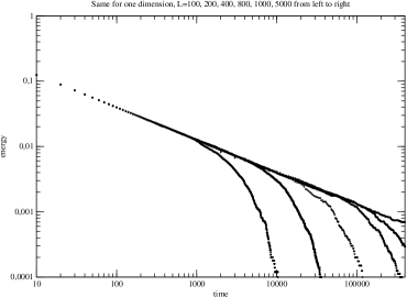
Figure 5: Same as Fig.4 but in one (top) or three (bottom) dimensions. Simulations shown for $d=1$ are done with random updating

Figure 6: Average over absolute difference between $x(t)$ and $x(t=0)=1/2)$ for $d=2$.

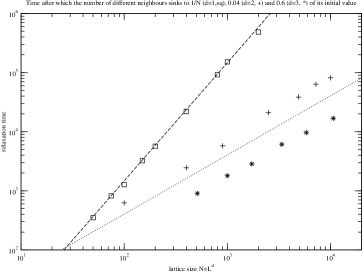
Figure 7: Time for the energy (= number of different lattice neighbours) to sink to some constant fraction of its initial value, versus population $N=L^{d}$, in one (+), two (x) and three (*) dimensions, from $x(t)$ averaged over 100 samples. Part a uses regular updating, part b the better random updating. The straight lines have slope 1 for $d=2,3$, and 2 for $d=1$.

The Abrams-Strogatz differential equation for the competition of a language Y with higher social status $1-s$ against another language X with lower social status $s$ is

$${\rm d}x/{\rm d}t=(1-x)x^{a}s-x(1-x)^{a}(1-s)$$

where $a\simeq 1.3$ [1] and $0<s\leq 1/2$. Here $x$ is the fraction in the population speaking language X with lower social status $s$ while the fraction $1-x$ speaks language Y. As initial condition we consider the situation in which both languages have the same number of speakers, $x(t=0)=1/2$. Figure 1 shows exponential decay for $a=1.31$ as well as for the simpler linear case $a=1$. For $s=1/2$ the symmetric situation $x=1/2$ is a stationary solution which is stable for $a<1$ and unstable for $a>1$. From now on we use $a=1$. This simplification makes the resulting differential equation

$${\rm d}x/{\rm d}t=(2s-1)(1-x)x$$

for $s\neq 1/2$ similar to the logistic equation which was applied to languages before, as reviewed by [16]. For $s=1/2$ any value of $x$ is a marginally stable stationary solution.

This differential equation is a mean-field approximation, ignoring the fate of individuals and the resulting fluctuations. We now put in $N$ individuals which in the fully connected model feel the influence of all individuals, while on the $d$-dimensional lattice they feel only the influence of their $2d$ nearest neighbors. The probability $p$ to switch from language Y to language X, and the probability $q$ for the inverse switch, are

$$p=x^{a}s,\quad q=(1-x)^{a}(1-s)\quad.$$

On a lattice, this $x$ is replaced by the fraction of X speakers in the neighborhood of $2d$ sites. We use regular updating for most of the results shown in this paper. Initially each person selects randomly one of the two languages with equal probability: $x(t=0)=0.5$. In the symmetric situation $s=1/2$ with $a=1$ that we will consider, our later lattice model becomes similar to the voter model [17].

Fig.2 shows our results for the fully connected case and Fig.3 for the square lattice with four neighbours; the results are quite similar to each other and to the original differential equation. A major difference with the differential equation (1) is seen in the symmetric case $s=1/2$ when the two languages are completely equivalent. Then the differential equation has $x$ staying at 1/2 for all times, while random fluctuation for finite population destabilize this situation and let one of the two languages win over the other, with $x$ going to zero or unity.

This latter case can be described in a unified way by looking at the number of lattice neighbours speaking a language different from the center site. It corresponds to an energy in the Ising magnet and measures microscopic interfaces. Initially this number equals $d$ on average, and then it decays to zero, first possibly as a power law, and then exponentially after a time which increases with increasing lattice size, Fig.4. The first decay describes a coarsening phenomenon, while the exponential decay is triggered by finite size fluctuations. In one dimension the initial decay follows a power law, $t^{-1/2}$, while in three dimensions an initial plateau is reached. This is followed by an exponential decay in $d=1,3$ as in two dimensions, Fig.5. Figure 6 shows that the average of $|x(t)-1/2|$ increases in two dimensions roughly as the square-root of time until it saturates at 1/2, indicating random walk behavior. (Note that first averaging over $x$ and then taking the absolute value $|<x>-1/2|$ would not give appropriate results since $<x>$ would always be 1/2 apart from fluctuations.)

In all the simulations described above, we went through the population regularly, like a typewriter on a square lattice, and for full connectivity kept the probabilities constant within each iteration. Using random updating is more realistic but takes more time. The long-time results are similar, and the power-law decay holds for $t<10^{2}$ with exponents 0.5 for $d=1$ (Fig. 5), and 0.1 (compatible with $1/\ln t$) for $d=2$. For $d=3$ a plateau is also reached. For the simpler regular updating we checked when the fraction $x$, initially 1/2, leaves the interval from 0.4 to 0.6 on its way to zero or one, Fig.7a. For the random updating we checked when the energy reaches a small fraction of its initial value, taken as $2/L$, $0.04$ and $0.6$ for $d=1,2,3$, Fig.7. Both figure parts are quite similar, with scaling laws for the characteristic time which are compatible with the ones obtained for a voter model [17]: $\tau\simeq N^{2}$ in $d=1$, $\tau\simeq N\ln N$ in $d=2$, and $\tau\simeq N$ in $d=3$, where $N=L^{d}$.

We conclude that agent-based simulations differ appreciably from the results from the mean-field approach for the symmetric case $s=1/2$: While Eqs.(1,2) then predict $x$ to stay at $x=1/2$, our simulations in Fig.4 and later show that after a decay everybody speaks the same language. In a fully connected network and in $d=3$ the decay is triggered by a finite size fluctuation, while in $d=1,2$ the intrinsic dynamics of the system causes an initial ordering phenomena in which spatial domains of speakers of the same language grow in size.

We acknowledge financial support form the MEC(Spain) through project CONOCE2 (FIS2004-00953).

References

- [1] D.M. Abrams and S.H. Strogatz, Nature 424 (2003) 900.
- [2] M. Patriarca and T. Leppänen, Physica A 338 (2004) 296.
- [3] W.S.Y. Wang and J.W. Minett, Trans. Philological Soc.103 (2005) 121 and unpublished.
- [4] J.Mira and A. Paredes, Europhys. Lett. 69 (2005) 1031.
- [5] J.P. Pinasco and L. Romanelli, Physica A 361 (2006) 355.
- [6] C. Schulze and D. Stauffer, Int. J. Mod. Phys. C 16 (2005) 781; Physics of Life Reviews 2 (2005) 89;
- [7] T. Tesileanu and H. Meyer-Ortmanns, Int. J. Mod. Phys. C 17, No. 3, 2006, in press.
- [8] D. Stauffer, C. Schulze, F.W.S. Lima, S. Wichmann and S. Solomon, e-print physics/0601160 at arXiv.org.
- [9] V.M. de Oliveira, M.A.F. Gomes and I.R. Tsang, Physica A 361 (2006) 361; V.M. de Oliveira, P.R.A. Campos, M.A.F. Gomes and I.R. Tsang, e-print physics/0510249 at arXiv.org for Physica A.
- [10] K. Kosmidis, J.M. Halley and P. Argyrakis, Physica A, 353 (2005) 595; K.Kosmidis, A. Kalampokis and P.Argyrakis, physics/0510019 in arXiv.org to be published in Physica A.
- [11] V. Schwämmle, Int. J. Mod. Phys. C 16 (2005) 1519; ibidem 17, No. 3, 2006, in press.
- [12] D. Stauffer, S. Moss de Oliveira, P.M.C. de Oliveira, J.S. Sa Martins, Biology, Sociology, Geology by Computational Physicists, Elsevier, Amsterdam 2006 in press.
- [13] C. Schulze and D. Stauffer, Comput. Sci. Engin. 8 (2006) in press.
- [14] M.A. Nowak, N.L. Komarova and P. Niyogi, Nature 417 (2002) 611.
- [15] A. Baronchelli, M. Felici, E. Caglioti, V. Loreto, L. Steels, e-prints physics/0509075, 0511201 and 0512045 at arXiv.org.
- [16] W.S.Y. Wang, J. Ke, J.W. Minett, in: Computational linguistics and beyond, eds. C.R. Huang and W. Lenders (Academica Sinica : Institute of Linguistics, Taipei, 2004); www.ee.cuhk.edu.hk/wsywang
- [17] R. Holley and T.M. Liggett, Ann. Probab. 3 (1975) 643; K. Suchecki, V.M. Eguíluz and M. San Miguel, Phys. Rev. E 72 (2005) 0361362 and Europhys. Lett. 69 (2005) 228; M. San Miguel, V.M. Eguíluz, R. Toral and K. Klemm, Comp. Sci. Engin. 7 (Nov/Dec 2005) 67.