Invariant imbedding theory of mode conversion in inhomogeneous plasmas. II. Mode conversion in cold, magnetized plasmas with perpendicular inhomogeneity

Abstract

A new version of the invariant imbedding theory for the propagation of coupled waves in inhomogeneous media is applied to the mode conversion of high frequency electromagnetic waves into electrostatic modes in cold, magnetized and stratified plasmas. The cases where the external magnetic field is applied perpendicularly to the direction of inhomogeneity and the electron density profile is linear are considered. Extensive and numerically exact results for the mode conversion coefficients, the reflectances and the wave electric and magnetic field profiles inside the inhomogeneous plasma are obtained. The dependences of mode conversion phenomena on the magnitude of the external magnetic field, the incident angle and the wave frequency are explored in detail.

I Introduction

Mode conversion from one type of wave mode to another type of mode at resonance points in an inhomogeneous plasma is a very important phenomenon in various branches of plasma physics.swanson ; budden ; ginz ; mjol In a previous paper,kim4 we embarked on a project of developing an exact theory of mode conversion in inhomogeneous plasmas, which is based on a new version of the invariant imbedding theory developed by us earlier.kim2 ; kim3 In that paper, we considered the mode conversion of the simplest kind, that is the conversion of obliquely-incident $p$-polarized electromagnetic waves into electrostatic plasma oscillations in cold, unmagnetized and stratified plasmas.piliya ; fors ; hink1 ; hink3 Using the invariant imbedding method,bell ; kly0 ; rammal ; kim1 ; lee ; lee2 we were able to calculate the mode conversion coefficient and the electromagnetic field distribution for linear and parabolic plasma density profiles in a numerically exact manner. In some cases, there were substantial discrepancies between our results and previous theoretical calculations.

The mode conversion phenomena in cold, unmagnetized plasmas are described by a single wave equation. A large number of wave propagation problems in more general situations, however, are described by two or more coupled wave equations. For the study of those problems, the invariant imbedding method needs to be generalized. This generalization was already made in Ref. 7 and has been successfully applied to various problems where several coupled waves propagate in inhomogeneous media. The propagation of electromagnetic waves in magnetized plasmas also involves several coupled waves. In this paper, we apply the theory developed in Ref. 7 to the mode conversion of high frequency electromagnetic waves into electrostatic modes in cold, magnetized and stratified plasmas.

Even in the relatively simple cases where the plasma is cold and stratified, the mode conversion of electromagnetic waves in magnetized plasmas is a highly complex problem. There are three independent directions in three-dimensional space, which are the directions of inhomogeneity, the external magnetic field and the incident wave vector. The wave propagation and mode conversion phenomena depend on the relative orientations of these three directions. In the present work, we limit our attention to one special configuration where the external magnetic field is applied perpendicularly to the direction of inhomogeneity and plane waves propagate in the plane spanned by the magnetic field and the inhomogeneity direction. Other configurations will be considered in forthcoming papers.

The theory developed in this paper can be applied easily to multi-species plasmas, which consist of electrons and different kinds of heavy ions. In this paper, we will consider only the propagation of high frequency waves and assume heavy ions to be immobile. Rather complicated, but very interesting mode conversion phenomena associated with low frequency waves and ion density oscillations will be subjects of our future publications.

Unlike in the unmagnetized case, the wave propagation in magnetized plasmas is anisotropic. In a uniform plasma where the wave vector is not precisely parallel to the external magnetic field, the ordinary (O) wave and the extraordinary (X) wave are two independent eigenmodes. When the wave frequency $\omega$ is bigger than the electron cyclotron frequency $\omega_{c}$, there can appear the O and X mode cutoffs and the X mode resonance inside the plasma. On the other hand, if the wave frequency is smaller than $\omega_{c}$, the O mode resonance can appear as well as the O and X mode cutoffs. In inhomogeneous plasmas, the O and X modes are no longer true eigenmodes and are coupled to each other. These modes can also be converted to upper hybrid oscillations at the resonances. The presence of both a strong coupling between different modes and the singularity associated with resonance points makes the solution of the mode conversion problem very difficult. As will be demonstrated later, our theory allows us to obtain an exact solution of this difficult problem in a remarkably simple and efficient manner.

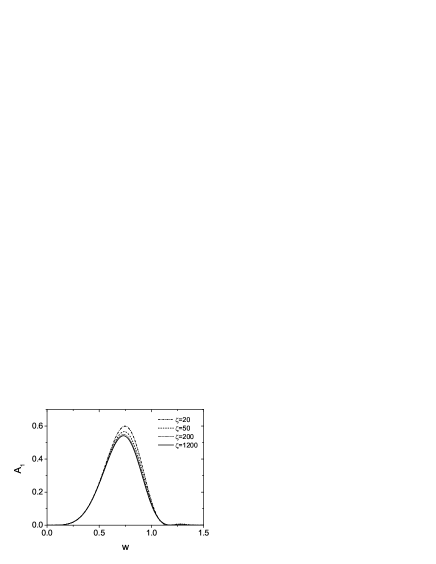
Figure 1: Mode conversion coefficient $A_{1}$ for normally-incident $s$ waves as a function of the parameter $w=\zeta^{1/3}\sqrt{Y}$ for several values of $\zeta=\omega\Lambda/c$ and for $\tilde{\nu}=10^{-8}$ and $L/\Lambda=20$. $A_{1}$ approaches a universal curve as $\zeta$ becomes large.

Mode conversion in magnetized plasmas has been studied extensively over several decades.piliya2 ; woo ; weitzner ; kitagawa ; window1 ; window2 ; wong ; maggs ; mjol3 ; mjol4 ; mjol2 ; seliga ; hansen ; johnson0 ; antani ; ueda ; yin ; golda ; kskim We will not attempt to give a detailed review of the literature here. Many of the previous works have used one approximation scheme or another, most frequently the WKB method. In a series of papers, Mjølhus calculated the mode conversion coefficient for cold, magnetized plasmas primarily using the WKB method.mjol3 ; mjol4 ; mjol2 This work, which was reviewed in Ref. 4 together with theoretical results of many other researchers, often predicts a complete mode conversion for certain parameters, in great contrast with our results. This discrepancy might be explained in large part by one crucial difference between Mjølhus’ and our calculations. In the present paper, we consider only the cases where linearly-polarized waves are incident from a vacuum onto a stratified plasma, whereas Mjølhus and other researchers have considered the cases where O or X waves are incident from a uniform plasma. Upon entering the plasma, linearly-polarized waves will be split into the O and X mode components. In the case of perpendicular inhomogeneity considered in this paper and when the waves are incident on a stratified plasma normally, mode conversion is caused solely by the X mode component. In this case, we find a perfect agreement between our result for incident $s$ waves shown in Fig. 1 and Mjølhus’ result for incident X waves. When the waves are incident obliquely and for sufficiently large values of the parameter $w$ defined in Sec. IV.1, mode conversion is dominated by the incident O mode. This case is closely related to the theory of radio windows in the ionosphere and magnetosphere.budden ; ginz ; mjol ; window1 ; window2 We find that the critical parameter values where the mode conversion coefficient takes the maximum value agrees extremely well with the analytical formula, Eq. (32), obtained by previous theories, for sufficiently large $w$. This is another evidence for the consistency between our theory and previous theories. For quantitative comparisons with previous results, we need to generalize our method to the cases where O or X waves are incident from a uniform plasma. This generalization will be pursued in future research. Since our theory is capable of producing exact results for realistic plasma density profiles, we expect it will be useful in the interpretation of various radio modification experiments.

In Sec. II, we present the details of a new version of the invariant imbedding theory for the propagation of coupled waves in stratified media. In Sec. III.1, we introduce the coupled wave equations for electromagnetic waves in cold, magnetized plasmas with perpendicular inhomogeneity. In Sec. III.2, we describe two linear plasma density profiles used for the calculations in this paper. The results of our calculations are presented in Sec. IV. In Sec. IV.1, we study the magnetic field dependence of mode conversion coefficients. In Sec. IV.2, we consider the dependence of mode conversion coefficients on the incident angle in detail. We also consider the spatial dependence of electric and magnetic field intensities. In Sec. IV.3, we discuss the frequency dependence of mode conversion coefficients. We conclude the paper in Sec. V. In Appendix A, we give a detailed derivation of Eq. (23).

II Invariant imbedding theory of the propagation of coupled waves in stratified media

In Ref. 7, we have developed a new version of the invariant imbedding theory for the propagation of coupled waves in arbitrarily-inhomogeneous stratified media. Since this theory will play a central role in our development of the theory of mode conversion, we give a detailed presentation of it here.

We consider $N$ coupled waves propagating in a stratified medium, where all physical parameters depend on only one spatial coordinate. We choose this coordinate as the $z$ axis and assume the inhomogeneous medium of thickness $L$ lies in $0\leq z\leq L$. We also assume that all waves propagate in the $xz$ plane. The $x$ component of the wave vector, $q$, is then a constant. In a large class of interesting problems, the wave equation of $N$ coupled waves in stratified media has the form

$${{d^{2}\psi}\over{dz^{2}}}-\frac{d\cal E}{dz}{\cal E}^{-1}(z)\frac{d\psi}{dz}+\left[{\cal E}(z)K^{2}{\cal M}(z)-q^{2}I\right]\psi=0,$$ (1)

where $\psi=(\psi_{1},\cdots,\psi_{N})^{T}$ is a vector wave function and ${\cal E}$ and ${\cal M}$ are $N\times N$ matrix functions. We assume that the waves are incident from a vacuum region where $z>L$ and transmitted to another vacuum region where $z<0$. $I$ is a unit matrix and $K$ is a diagonal matrix such that $K_{ij}=k_{i}\delta_{ij}$, where $k_{i}$ is the magnitude of the vacuum wave vector for the $i$-th wave. In the problem considered in this paper, all $k_{i}$’s are equal. However, there exist many cases where $k_{i}$’s take different values. It is useful to rewrite Eq. (1) as

$$\frac{d}{dz}\left[{\cal E}^{-1}(z){{d\psi}\over{dz}}\right]+\left[K^{2}{\cal M}(z)-q^{2}{\cal E}^{-1}(z)\right]\psi=0.$$ (2)

From this form, we can see that ${\cal E}^{-1}d\psi/dz$ is continuous everywhere except at some singular points.

Eq. (1) is suitable when the matrices ${\cal E}$ and ${\cal M}$ do not contain the constant $q$. In the cases where the $q$ dependence cannot be separated as simply as in Eq. (1), it is more convenient to write the wave equation as

$${{d^{2}\psi}\over{dz^{2}}}-\frac{d\cal E}{dz}{\cal E}^{-1}(z)\frac{d\psi}{dz}+{\cal E}(z)K^{2}{\cal M}(z)\psi=0$$ (3)

and define ${\cal E}$ and ${\cal M}$ as $q$-dependent quantities. By assigning ${\cal E}(z)$ and ${\cal M}(z)$ suitably, we are able to describe various kinds of waves in a number of stratified media using either Eq. (1) or (3). A wide variety of mode conversion phenomena observed in space and laboratory plasmas can be studied using these equations.

We generalize Eqs. (1) and (3) slightly, by replacing the vector wave function $\psi$ by an $N\times N$ matrix wave function $\Psi$, the $j$-th column vector $(\Psi_{1j},\cdots,\Psi_{Nj})^{T}$ of which represents the wave function when the incident wave consists only of the $j$-th wave of unit amplitude. Our main interest is in the reflection and transmission coefficient matrices $r=r(L)$ and $t=t(L)$. The wave function in the incident and transmissive regions are expressed in terms of $r$ and $t$:

$$\Psi(z)=\left\{\begin{array}[]{ll}e^{iP(L-z)}+e^{iP(z-L)}~{}r,&~{}z>L\\ e^{-iPz}~{}t,&~{}z<0\end{array}\right.,$$ (6)

where $P$ is a diagonal matrix satisfying $P_{ij}=p_{i}\delta_{ij}$ and $p_{i}$ is the negative $z$ component of the vacuum wave vector for the $i$-th wave. It is important to write the products of two matrices, $e^{iP(z-L)}~{}r$ and $e^{-iPz}~{}t$, in the given order. From Eq. (6), we obtain $\Psi(L)=I+r$ and $\Psi(0)=t$.

Let us introduce a matrix

$$g(z,z^{\prime})=\left\{\begin{array}[]{ll}{\mathcal{T}}\exp\left[i\int_{z^{\prime}}^{z}dz^{\prime\prime}~{}{\cal E}(z^{\prime\prime})P\right],&~{}z>z^{\prime}\\ \tilde{\mathcal{T}}\exp\left[-i\int_{z^{\prime}}^{z}dz^{\prime\prime}~{}{\cal E}(z^{\prime\prime})P\right],&~{}z<z^{\prime}\end{array}\right.$$ (9)

where $\mathcal{T}$ and $\tilde{\mathcal{T}}$ are the time-ordering and anti-time-ordering operators respectively. When applied to a product of matrices which are functions of $z$, $\mathcal{T}$ ($\tilde{\mathcal{T}}$) arranges the matrices in the order of decreasing (increasing) $z$. For instance, $\mathcal{T}\left[{\cal E}(z_{1}){\cal E}(z_{2})\right]={\cal E}(z_{2}){\cal E}(z_{1})$ and $\tilde{\mathcal{T}}\left[{\cal E}(z_{2}){\cal E}(z_{1})\right]={\cal E}(z_{1}){\cal E}(z_{2})$, if $z_{2}>z_{1}$. Though, strictly speaking, $\mathcal{T}$ has to be called a space-ordering operator, we keep using the standard terminology, time-ordering operator, commonly used in quantum mechanics.qm Expanding the matrix exponentials in Eq. (9) in a Taylor series and using the definitions of $\mathcal{T}$ and $\tilde{\mathcal{T}}$, we can easily prove that $g(z,z^{\prime})$ satisfies the differential equations

$$\frac{\partial}{\partial z}g(z,z^{\prime}) = i~{}{\rm sgn}(z-z^{\prime})~{}{\mathcal{E}}(z)Pg(z,z^{\prime}),$$

$$\frac{\partial}{\partial z^{\prime}}g(z,z^{\prime}) = -i~{}{\rm sgn}(z-z^{\prime})~{}g(z,z^{\prime}){\mathcal{E}}(z^{\prime})P.$$ (10)

Using Eqs. (9) and (10), the wave equation (1) is transformed exactly to an integral equation

$$\Psi(z,L)=g(z,L)$$

$$~{}~{}-{i\over 2}\int_{0}^{L}dz^{\prime}g(z,z^{\prime})\left[{\cal E}(z^{\prime})P-P{\cal M}(z^{\prime})-q^{2}P^{-1}{\cal M}(z^{\prime})+q^{2}P^{-1}{\cal E}^{-1}(z^{\prime})\right]\Psi(z^{\prime},L),$$ (11)

where we have considered $\Psi$ as a function of both $z$ and $L$. We replace $L$ by a variable $l$ and take a derivative of this equation with respect to $l$. Then we obtain

$$\frac{\partial\Psi(z,l)}{\partial l}=i\Psi(z,l)\alpha(l)+\Phi(z,l),$$ (12)

where

$$\alpha(l)={\cal E}(l)P-{1\over 2}\left[{\cal E}(l)P-P{\cal M}(l)-q^{2}P^{-1}{\cal M}(l)+q^{2}P^{-1}{\cal E}^{-1}(l)\right]\Psi(l,l),$$

$$\Phi(z,l)=-{i\over 2}\int_{0}^{l}dz^{\prime}g(z,z^{\prime})\left[{\cal E}(z^{\prime})P-P{\cal M}(z^{\prime})-q^{2}P^{-1}{\cal M}(z^{\prime})+q^{2}P^{-1}{\cal E}^{-1}(z^{\prime})\right]\Phi(z^{\prime},l).$$ (13)

We notice that $\Phi(z,l)$ satisfies an equation similar to Eq. (11) except that there is no source term (that is, $g(z,l)$). This implies $\Phi(z,l)=0$ and then we have

$$\frac{\partial\Psi(z,l)}{\partial l}=i\Psi(z,l)\alpha(l).$$ (14)

Taking now the derivative of $\Psi(l,l)$ with respect to $l$, we obtain

$$\frac{d\Psi(l,l)}{dl} = \frac{\partial\Psi(z,l)}{\partial z}\Bigg{|}_{z=l}+\frac{\partial\Psi(z,l)}{\partial l}\Bigg{|}_{z=l}$$ (15)

$$= i{\cal E}(l)P\left[r(l)-I\right]+i\Psi(l,l)\alpha(l),$$

where we have used Eq. (14) and the fact that ${\mathcal{E}}^{-1}(z)~{}\partial\Psi(z,l)/\partial z$ is continuous at $z=l$. Since $\Psi(l,l)=I+r(l)$, we find the invariant imbedding equation satisfied by $r(l)$:

$${{dr}\over{dl}} = i\left[r(l){\cal E}(l)P+{\cal E}(l)Pr(l)\right]$$ (16)

$$-{i\over 2}[r(l)+I]\left[{\cal E}(l)P-P{\cal M}(l)-q^{2}P^{-1}{\cal M}(l)+q^{2}P^{-1}{\cal E}^{-1}(l)\right][r(l)+I].$$

Similarly by setting $z=0$ in Eq. (14), we find the invariant imbedding equation for $t(l)$ ($=\Psi(0,l)$):

$${{dt}\over{dl}} = it(l){\cal E}(l)P$$ (17)

$$-{i\over 2}t(l)\left[{\cal E}(l)P-P{\cal M}(l)-q^{2}P^{-1}{\cal M}(l)+q^{2}P^{-1}{\cal E}^{-1}(l)\right][r(l)+I].$$

These equations are supplemented with the initial conditions, $r(0)=0$ and $t(0)=I$.

We integrate the coupled differential equations (16) and (17) numerically from $l=0$ to $l=L$ using the initial conditions and obtain the reflection and transmission coefficient matrices $r$ and $t$ as functions of $L$. The invariant imbedding method can also be used in calculating the field amplitude $\Psi(z)$ inside the inhomogeneous medium. Rewriting Eq. (14), we get

$${{\partial\Psi(z,l)}\over{\partial l}} = i\Psi(z,l){\cal E}(l)P$$ (18)

$$-{i\over 2}\Psi(z,l)\left[{\cal E}(l)P-P{\cal M}(l)-q^{2}P^{-1}{\cal M}(l)+q^{2}P^{-1}{\cal E}^{-1}(l)\right][r(l)+I].$$

For a given $z$ ($0<z<L$), the field amplitude $\Psi(z,L)$ is obtained by integrating this equation from $l=z$ to $l=L$ using the initial condition $\Psi(z,z)=I+r(z)$.

Our invariant imbedding equations, Eqs. (16-18), have been applied successfully to the study of the propagation of electromagnetic waves in multilayer systems made of chiral media and of phase-conjugating media.kim3

III Coupled wave equations for cold, magnetized plasmas with perpendicular inhomogeneity

III.1 Coupled wave equations

Eqs. (16), (17) and (18) are the starting point in our exact analysis of a variety of wave coupling and mode conversion phenomena. In the rest of this paper, we apply these equations to the high frequency wave propagation and mode conversion in cold, magnetized plasmas. For the sake of simplicity, we restrict our attention to the cases where the external magnetic field is applied perpendicularly to the direction of inhomogeneity.

We assume that the plasma density varies only in the $z$ direction and the uniform external magnetic field ${\bf B}_{0}$ ($=B_{0}\hat{\bf x}$) is directed in the $x$ direction. The cold plasma dielectric tensor, $\epsilon$, for high frequency waves in the present geometry is written as

$$\epsilon=\pmatrix{\epsilon_{3}&0&0\cr 0&\epsilon_{1}&i\epsilon_{2}\cr 0&-i\epsilon_{2}&\epsilon_{1}},$$ (19)

where

$$\epsilon_{1} = 1-\frac{\omega_{p}^{2}\left(\omega+i\nu\right)}{\omega\left[\left(\omega+i\nu\right)^{2}-\omega_{c}^{2}\right]},$$

$$\epsilon_{2} = \frac{\omega_{p}^{2}\omega_{c}}{\omega\left[\left(\omega+i\nu\right)^{2}-\omega_{c}^{2}\right]},$$

$$\epsilon_{3} = 1-\frac{\omega_{p}^{2}}{\omega\left(\omega+i\nu\right)}.$$ (20)

We note that the indices 1, 2 and 3 in $\epsilon_{1}$, $\epsilon_{2}$ and $\epsilon_{3}$ have no direct relationship with the spatial coordinates $x$, $y$ and $z$. The constant $\nu$ is the phenomenological collision frequency. In Gaussian units, the electron plasma frequency $\omega_{p}$ and the electron cyclotron frequency $\omega_{c}$ are given by

$$\omega_{p}^{2}=\frac{4\pi e^{2}}{m_{e}}n(z),~{}~{}~{}\omega_{c}=\frac{eB_{0}}{m_{e}c},$$ (21)

where $m_{e}$ and $-e$ are the electron mass and charge respectively. The spatial inhomogeneity of plasmas enters through the $z$ dependence of the electron number density $n$.

For monochromatic waves of frequency $\omega$, the wave equations satisfied by the electric and magnetic fields in cold, magnetized plasmas have the form

$$-\nabla\times\left(\nabla\times{\bf E}\right)+{\omega^{2}\over c^{2}}\epsilon\cdot{\bf E}=0,$$

$$-\nabla\times\left(\epsilon^{-1}\cdot\nabla\times{\bf B}\right)+{\omega^{2}\over c^{2}}{\bf B}=0.$$ (22)

In this paper, we restrict our interest to the cases where plane waves propagate parallel to the $xz$ plane, which is sometimes called the magnetic meridian plane. We assume that all field components depend on $x$ and $t$ through a factor $e^{i[(k\sin\theta)x-\omega t]}$, where $k=\omega/c$ and $\theta$ is the incident angle, and have no $y$ dependence. In this situation, we can eliminate $E_{x}$, $E_{z}$, $B_{x}$ and $B_{z}$ from Eq. (22) and obtain two coupled wave equations satisfied by the $z$-dependent field amplitudes $E_{y}=E_{y}(z)$ and $B_{y}=B_{y}(z)$, which turn out to have precisely the same form as Eq. (3) with

$$\psi=\pmatrix{E_{y}\cr B_{y}\cr},~{}~{}K=\frac{\omega}{c}I,$$

$${\cal E}=\pmatrix{1&0\cr 0&\epsilon_{3}\cr},$$

$${\cal M}=\pmatrix{\epsilon_{1}-\frac{{\epsilon_{2}}^{2}}{\epsilon_{1}}-\sin^{2}\theta&-i{\epsilon_{2}\over\epsilon_{1}}\sin\theta\cr i{\epsilon_{2}\over\epsilon_{1}}\sin\theta&1-\frac{\sin^{2}\theta}{\epsilon_{1}}\cr}.$$ (23)

A derivation of this crucial result is given in Appendix A.

We use Eqs. (16), (17) and (23) in calculating the reflection and transmission coefficients. In our notation, $r_{11}$ ($r_{21}$) is the reflection coefficient when the incident wave is $E_{y}$ (that is, $s$-polarized) and the reflected wave is $E_{y}$ ($B_{y}$). Similarly, $r_{22}$ ($r_{12}$) is the reflection coefficient when the incident wave is $B_{y}$ (that is, $p$-polarized) and the reflected wave is $B_{y}$ ($E_{y}$). Similar definitions are applied to the transmission coefficients. The reflectances and transmittances are defined by $R_{ij}=|r_{ij}|^{2}$ and $T_{ij}=|t_{ij}|^{2}$. When the dielectric permittivities of the incident region and the transmissive region are the same, we can calculate the wave absorption by $A_{j}\equiv 1-R_{1j}-R_{2j}-T_{1j}-T_{2j}$ ($j=1,2$). If a mode conversion occurs, this quantity is nonzero even in the limit where the damping constant $\nu$ goes to zero.kim4 In that limit, we will call $A_{j}$ as the mode conversion coefficient.

Finally, we use Eqs. (18) and (23) in calculating the electromagnetic field amplitudes $E_{y}(z)$ and $B_{y}(z)$ inside the inhomogeneous region. Once we obtain $E_{y}$ and $B_{y}$, we can use Eq. (36) to calculate other field components $E_{x}$, $E_{z}$, $B_{x}$ and $B_{z}$.

III.2 Plasma density profiles

Our theory can be applied to any function $n(z)$ for the electron density profile. In the present work, we confine our calculations to two kinds of linear profiles. In the first one, we assume that the density is given by

$$n(z)=\left\{\begin{array}[]{ll}0&~{}~{}\mbox{if $z>L$}\\ n_{0}\frac{L-z}{\Lambda}&~{}~{}\mbox{if $0\leq z\leq L$}\\ 0&~{}~{}\mbox{if $z<0$}\end{array}\right.,$$ (24)

where the constant $\Lambda$ is the scale length for the linear density profile, and the wave frequency is fixed at the value of the local plasma frequency at $z=L-\Lambda$, that is $\omega=(4\pi n_{0}e^{2}/m_{e})^{1/2}$. In this case, the dielectric tensor for $0\leq z\leq L$ is given by Eq. (19) with

$$\epsilon_{1} = 1-\frac{L-z}{\Lambda}\frac{1+i\tilde{\nu}}{\left(1+i\tilde{\nu}\right)^{2}-Y^{2}},$$

$$\epsilon_{2} = \frac{L-z}{\Lambda}\frac{Y}{\left(1+i\tilde{\nu}\right)^{2}-Y^{2}},$$

$$\epsilon_{3} = 1-\frac{L-z}{\Lambda}\frac{1}{1+i\tilde{\nu}},$$ (25)

where $\tilde{\nu}\equiv\nu/\omega$ and $Y\equiv\omega_{c}/\omega$. For $z>L$ or $z<0$, the dielectric tensor is equal to a unit matrix. We will use this tensor in studying the dependencies of various quantities on the incident angle and the strength of the external magnetic field.

We are also interested in the frequency dependence of mode conversion phenomena. For this purpose, we consider a linear density profile for $0\leq z\leq L$ such that the plasma frequency satisfies

$$\omega_{p}=2\pi f_{0}\left[1+24\left(1-\frac{z}{L}\right)\right]^{1/2},$$ (26)

where $f_{0}$ is the local (nonangular) plasma frequency at $z=L$ measured in MHz. We introduce nonangular frequencies

$$f\equiv\frac{\omega}{2\pi},~{}~{}f_{c}\equiv\frac{\omega_{c}}{2\pi},~{}~{}f_{\nu}\equiv\frac{\omega_{\nu}}{2\pi},$$ (27)

also measured in MHz. Then, for $0\leq z\leq L$, the dielectric tensor is given by Eq. (19) with

$$\epsilon_{1} = 1-\frac{f_{0}^{2}\left(f+if_{\nu}\right)}{f\left[\left(f+if_{\nu}\right)^{2}-f_{c}^{2}\right]}\left[1+24\left(1-\frac{z}{L}\right)\right],$$

$$\epsilon_{2} = \frac{f_{0}^{2}f_{c}}{f\left[\left(f+if_{\nu}\right)^{2}-f_{c}^{2}\right]}\left[1+24\left(1-\frac{z}{L}\right)\right],$$

$$\epsilon_{3} = 1-\frac{f_{0}^{2}}{f\left(f+if_{\nu}\right)}\left[1+24\left(1-\frac{z}{L}\right)\right].$$ (28)

If $z>L$ or $z<0$, the dielectric tensor is equal to a unit matrix. For specific calculations, we will assume $f_{0}=1$ MHz and $f_{c}=1.5$ MHz. Then the local plasma frequency varies from 1 MHz at $z=L$ to 5 MHz at $z=0$.

IV Results

IV.1 Magnetic field dependence

In this subsection, we study the dependence of mode conversion coefficients on the magnitude of the external magnetic field $B_{0}$, or equivalently on the cyclotron frequency $\omega_{c}$. We first consider the simplest case where linearly-polarized plane waves are incident normally (i.e. $\theta=0$) on a layer of inhomogeneous plasma with the linear density profile given by Eq. (24). In this case, it is well-known that there is a resonance associated with X waves if the wave frequency is equal to the upper hybrid frequency $\omega_{uh}=(\omega_{p}^{2}+\omega_{c}^{2})^{1/2}$, whereas there is no resonance associated with O waves. For $L>\Lambda$, the resonance condition $\omega=\omega_{uh}$ can be satisfied if $Y<1$ (i.e. $\omega>\omega_{c}$). The coordinate of the resonance point $z_{R}$ is given by

$$z_{R}=L-\Lambda\left(1-Y^{2}\right).$$ (29)

Since we are considering the cases where waves are incident from a vacuum region, we assume that the incident wave is either $s$- or $p$-polarized. In the case of normal incidence, $p$ waves are the same as O waves and $s$ waves are similar to X waves. Therefore we expect that there is no mode conversion when $p$ waves are incident normally, whereas some portion of normally-incident $s$ waves will convert to upper hybrid oscillations.

Actual calculations using our invariant imbedding theory show that the $p$ wave absorption $A_{2}$ vanishes indeed when the damping constant $\tilde{\nu}$ is very small. In Fig. 1, we plot the $s$ wave mode conversion coefficient $A_{1}$ as a function of the dimensionless parameter $w\equiv\zeta^{1/3}\sqrt{Y}$ ($\propto\sqrt{B_{0}}$) for several values of $\zeta\equiv\omega\Lambda/c$ and for $\theta=0$, $\tilde{\nu}=10^{-8}$ and $L/\Lambda=20$. We notice that $A_{1}$ approaches a universal curve as $\zeta$ increases to large values. We find this universal curve agrees remarkably well with Fig. 4 presented in Ref. 4.

Next we consider the cases where linearly-polarized waves are incident obliquely at an angle $\theta$. In those cases, both $s$ and $p$ waves can generate X mode components inside the inhomogeneous plasma and be converted to upper hybrid oscillations at $z=z_{R}$. In Fig. 2, we show the $s$ ($p$) wave mode conversion coefficient $A_{1}$ ($A_{2}$) as a function of $w$ for several values of the parameter $v\equiv\zeta^{1/3}\sin\theta$ and for $\zeta=500$, $\tilde{\nu}=10^{-8}$ and $L/\Lambda=20$. As the incident angle increases, $A_{2}$ grows from zero to finite values.

In Fig. 3, we plot the reflectances $R_{11}$, $R_{22}$ and $R_{12}$ for $\zeta=500$, $\tilde{\nu}=10^{-8}$ and $L/\Lambda=20$. The parameter $v$ is equal to 1 in Fig. 3(a) and 2 in Fig. 3(b). It can be proved that $R_{21}$ is always identical to $R_{12}$. We observe that in the parameter region where there is no mode conversion, the reflectances are rapidly oscillating functions of $w$.

IV.2 Incident angle dependence and the electromagnetic field distribution

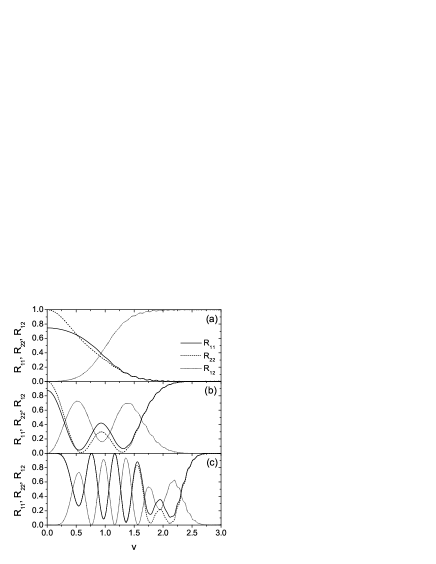
Figure 5: Reflectances $R_{11}$, $R_{22}$ and $R_{12}$ ($=R_{21}$) as a function of $v$ for $\zeta=500$, $\tilde{\nu}=10^{-8}$, $L/\Lambda=20$ and (a) $w=0.5$, (b) $w=1$, (c) $w=2$.

In this subsection, we consider the dependence of mode conversion coefficients on the incident angle $\theta$ in detail. We also consider the spatial dependence of electric and magnetic field intensities associated with the electromagnetic wave. In Fig. 4, we show the $s$ ($p$) wave mode conversion coefficient $A_{1}$ ($A_{2}$) as a function of the parameter $v$, which is proportional to $\sin\theta$, for several values of $w$ and for $\zeta=500$, $\tilde{\nu}=10^{-8}$ and $L/\Lambda=20$. In the absence of the external magnetic field, the $s$ wave mode conversion coefficient $A_{1}$ vanishes, whereas the $p$ wave mode conversion coefficient $A_{2}$ agrees with the result for unmagnetized cases reported in Ref. 7. When $B_{0}>0$, $A_{1}$ becomes nonzero. For $w$ values well over 1, mode conversion occurs in a narrow range of $v$ or $\theta$. This range is called the radio window and becomes narrower as $w$ or $\zeta$ increases. In Fig. 5, we plot the reflectances $R_{11}$, $R_{22}$ and $R_{12}$ for $\zeta=500$, $\tilde{\nu}=10^{-8}$ and $L/\Lambda=20$. The parameter $w$ is equal to 0.5 in Fig. 5(a), 1 in Fig. 5(b) and 2 in Fig. 5(c).

The occurrence of radio windows is closely related to the coupling between the O mode and the X mode near the position where $\omega=\omega_{p}$, which has the coordinate $z=L-\Lambda$ ($\equiv z_{0}$) in our profile. It is well-known that this coupling is most efficient when the incident angle satisfies

$$\sin\theta=\pm\sqrt{\frac{Y}{Y+1}}\sin\alpha$$ (30)

for $Y<1$, or

$$\sin\theta=\pm\sqrt{\frac{Y}{Y-1}}\sin\alpha$$ (31)

for $Y>1$, where $\alpha$ is the angle between the external magnetic field and the direction of inhomogeneity and is equal to $90^{\circ}$ in our case.budden ; ginz ; mjol ; window1 ; mjol2 ; seliga Then it is easy to see that there is no incident angle satisfying Eq. (31) and that Eq. (30) can be rewritten as

$$v=\frac{w}{\sqrt{1+w^{2}/\zeta^{2/3}}},$$ (32)

where we have kept only the plus sign.

In Fig. 6(a), we plot $v_{1,{\rm max}}$ and $v_{2,{\rm max}}$, which are the $v$ values where $A_{1}$ and $A_{2}$ take the maximum values $A_{1,{\rm max}}$ and $A_{2,{\rm max}}$ respectively in Fig. 4, versus $w$ for $\zeta=500$, $\tilde{\nu}=10^{-8}$ and $L/\Lambda=20$ and compare them with Eq. (32). We find that when $w$ is greater than about 1, the agreement between our result and Eq. (32) is excellent. When $w<1$, however, our result differs greatly from Eq. (32). In Fig. 6(b), the maximum mode conversion coefficients $A_{1,{\rm max}}$ and $A_{2,{\rm max}}$ are plotted versus $w$.

In the rest of this subsection, we consider the spatial dependence of electric and magnetic field intensities inside the inhomogeneous plasma. Using Eqs. (18) and (23), we have calculated the electric and magnetic field components $E_{y1}(z)$ and $B_{y1}(z)$ for incident $s$ waves and $E_{y2}(z)$ and $B_{y2}(z)$ for incident $p$ waves. In Fig. 7, we plot the absolute values of $E_{y1}(z)$, $B_{y1}(z)$, $E_{y2}(z)$ and $B_{y2}(z)$ for $\zeta=50$, $\tilde{\nu}=10^{-3}$ and $L/\Lambda=20$. $v$ is chosen to be equal to the critical value $v_{c}\equiv w/\sqrt{1+w^{2}/\zeta^{2/3}}$ and the value of $w$ is 1 in Figs. 7(a-d), 2 in Figs. 7(e-h) and 3 in Figs. 7(i-l). On these figures, we also indicate the positions of the resonant point $z_{R}$ given by Eq. (29) and the point $z_{c}$ where incident waves start to become evanescent when Eq. (32) is satisfied. $z_{c}$ turns out to be given by

$$z_{c}-z_{0}=\Lambda\frac{2Y}{1+Y},$$ (33)

where $Y=w^{2}/\zeta^{2/3}$. For $z_{R}<z<z_{c}$, electromagnetic waves are expected to be evanescent. The highly oscillating behavior for $z<z_{R}$ in Figs. 7(i-l) comes from a branch of the X mode commonly known as the Z mode.

In Fig. 8, we compare the field distributions at the critical value of $v$ given by Eq. (32) with those for $v$ slightly different from the critical value. In Figs. 8(e-h), $\zeta=50$, $\tilde{\nu}=10^{-3}$, $L/\Lambda=20$, $w=3$ and $v=v_{c}\approx 2.326$. $v$ is equal to $v_{c}-0.1$ in Figs. 8(a-d) and $v_{c}+0.1$ in Figs. 8(i-l) and all other parameters are the same as in Figs. 8(e-h). We find that the evanescent behavior is absent in off-critical cases.

In Fig. 9, we show the absolute values of the $z$ components of the electric field, $E_{z1}$ for incident $s$ waves and $E_{z2}$ for incident $p$ waves, calculated using Eq. (36). The parameters used are $\zeta=50$, $\tilde{\nu}=10^{-3}$, $L/\Lambda=20$, $w=3$ and $v=v_{c}$ for Figs. 9(c-d), $v=v_{c}-0.3$ for Figs. 9(a-b), $v=v_{c}+0.3$ for Figs. 9(e-f). In off-critical cases, the evanescent behavior is absent and the divergence at the resonance point becomes weaker.

IV.3 Frequency dependence

For the study of the frequency dependence of mode conversion phenomena, we use the plasma density profile given by Eq. (26). We assume $f_{0}=1$ MHz, so the local plasma frequency varies from 1 MHz at $z=L$ to 5 MHz at $z=0$. The cyclotron frequency $f_{c}$ is 1.5 MHz and the collision frequency $f_{\nu}$ is equal to $10^{-8}$ MHz. We show the mode conversion coefficients $A_{1}$ and $A_{2}$ for several incident angles and for $L=250$ m in Fig. 10 and for $L=1500$ m in Fig. 11. In all cases, mode conversion is found to occur only in the frequency range determined by the upper hybrid frequency. In other words, $A_{1}$ and $A_{2}$ are nonzero only for $\sqrt{1^{2}+1.5^{2}}\approx 1.8~{}{\rm MHz}<f<\sqrt{5^{2}+1.5^{2}}\approx 5.22~{}{\rm MHz}$.

In the case of uniform magnetized plasmas, the O (X) wave shows a resonance when the wave frequency $\omega$ is equal to the resonance frequency $\omega_{O}$ ($\omega_{X}$). The frequencies $\omega_{O}$ and $\omega_{X}$ are given by

$$\omega_{O}\equiv\sqrt{\frac{\omega_{p}^{2}+\omega_{c}^{2}}{2}-\sqrt{\left(\frac{\omega_{p}^{2}+\omega_{c}^{2}}{2}\right)^{2}-\omega_{p}^{2}\omega_{c}^{2}\cos^{2}\phi}},$$

$$\omega_{X}\equiv\sqrt{\frac{\omega_{p}^{2}+\omega_{c}^{2}}{2}+\sqrt{\left(\frac{\omega_{p}^{2}+\omega_{c}^{2}}{2}\right)^{2}-\omega_{p}^{2}\omega_{c}^{2}\cos^{2}\phi}},$$ (34)

where $\phi$ is the angle between the external magnetic field and the wave vector.budden The fact that mode conversion occurs only when $\omega$ is equal to $\omega_{uh}$ regardless of the incident angle suggests that in our stratified plasma, only the X wave component propagating in the direction of inhomogeneity with $\phi=90^{\circ}$ can cause mode conversion.

V Conclusion

In this paper, we have presented a new version of the invariant imbedding theory for the propagation of coupled waves in inhomogeneous media and applied it to the mode conversion of high frequency electromagnetic waves into electrostatic modes in cold, magnetized and stratified plasmas. We have considered the cases where the external magnetic field is applied perpendicularly to the direction of inhomogeneity and the electron density profile is linear. We have obtained extensive and numerically exact results for the mode conversion coefficients, the reflectances and the wave electric and magnetic field profiles inside the inhomogeneous plasma. We have explored the dependences of mode conversion phenomena on the size of the external magnetic field, the incident angle and the wave frequency in detail. Our theoretical method and results are expected to be quite useful in investigating a broad range of observations and experiments on the interaction between electromagnetic waves and plasmas both in space and laboratories. In forthcoming papers, we will apply our theory to the cases where the external magnetic field is applied in different directions and to the propagation and mode conversion of low frequency waves in more general plasmas consisting of various kinds of ions as well as electrons.

Appendix A Derivation of the matrices $\mathcal{E}$ and $\mathcal{M}$

Using the Maxwell’s equations

$$\nabla\times{\bf E}=-{1\over c}{{\partial{\bf B}}\over{\partial t}}=ik{\bf B},$$

$$\nabla\times{\bf B}={1\over c}{{\partial{\bf D}}\over{\partial t}}=-ik\epsilon\cdot{\bf E}$$ (35)

and the dielectric tensor, Eq. (19), we express the $z$-dependent field amplitudes $E_{x}$, $E_{z}$, $B_{x}$ and $B_{z}$ in terms of $E_{y}$ and $B_{y}$:

$$E_{x}(z)=-\frac{i}{k\epsilon_{3}(z)}{B_{y}}^{\prime}(z),$$

$$E_{z}(z)=i\frac{\epsilon_{2}(z)}{\epsilon_{1}(z)}E_{y}(z)-\frac{\sin\theta}{\epsilon_{1}(z)}B_{y}(z),$$

$$B_{x}(z)=\frac{i}{k}{E_{y}}^{\prime}(z),$$

$$B_{z}(z)=E_{y}(z)\sin\theta,$$ (36)

where the prime denotes a differentiation with respect to $z$. We substitute these equations and their derivatives into the $z$ components of Eq. (22) and obtain a matrix equation of the form

$$\psi^{\prime\prime}+{\mathcal{A}}\psi^{\prime}+{\mathcal{B}}\psi=0,$$ (37)

where

$$\psi=\pmatrix{E_{y}(z)\cr B_{y}(z)\cr},~{}~{}{\mathcal{A}}=\pmatrix{0&0\cr 0&-\frac{{\epsilon_{3}}^{\prime}(z)}{\epsilon_{3}(z)}\cr},$$

$${\mathcal{B}}=k^{2}\pmatrix{\epsilon_{1}(z)-\frac{\left[\epsilon_{2}(z)\right]^{2}}{\epsilon_{1}(z)}-\sin^{2}\theta&-i{\epsilon_{2}(z)\over\epsilon_{1}(z)}\sin\theta\cr i{\epsilon_{2}(z)\epsilon_{3}(z)\over\epsilon_{1}(z)}\sin\theta&\epsilon_{3}(z)\left[1-\frac{\sin^{2}\theta}{\epsilon_{1}(z)}\right]\cr}.$$ (38)

Comparing this with Eq. (3), we get ${\mathcal{A}}=-{\cal E}^{\prime}{\cal E}^{-1}$ and ${\mathcal{B}}={\cal E}K^{2}{\cal M}=k^{2}{\cal E}{\cal M}$ with $K=kI$. From the forms of $\mathcal{A}$ and $\mathcal{B}$, we deduce the matrices

$${\cal E}=\pmatrix{1&0\cr 0&\epsilon_{3}\cr},$$

$${\cal M}=\pmatrix{\epsilon_{1}-\frac{{\epsilon_{2}}^{2}}{\epsilon_{1}}-\sin^{2}\theta&-i{\epsilon_{2}\over\epsilon_{1}}\sin\theta\cr i{\epsilon_{2}\over\epsilon_{1}}\sin\theta&1-\frac{\sin^{2}\theta}{\epsilon_{1}}\cr}$$ (39)

in a straightforward manner.

Figure 2: Mode conversion coefficient $A_{1}$ ($A_{2}$) for obliquely-incident $s$ ($p$) waves as a function of $w$ for several values of $v=\zeta^{1/3}\sin\theta$ and for $\zeta=500$, $\tilde{\nu}=10^{-8}$ and $L/\Lambda=20$.

Figure 3: Reflectances $R_{11}$, $R_{22}$ and $R_{12}$ ($=R_{21}$) as a function of $w$ for $\zeta=500$, $\tilde{\nu}=10^{-8}$, $L/\Lambda=20$ and (a) $v=1$, (b) $v=2$.

Figure 4: Mode conversion coefficients $A_{1}$ and $A_{2}$ as a function of $v$ for several values of $w$ and for $\zeta=500$, $\tilde{\nu}=10^{-8}$ and $L/\Lambda=20$.

Figure 6: (a) $v_{1,{\rm max}}$ ($v_{2,{\rm max}}$), which is the $v$ value where $A_{1}$ ($A_{2}$) takes the maximum value $A_{1,{\rm max}}$ ($A_{2,{\rm max}}$) in Fig. 4, as a function of $w$ for $\zeta=500$, $\tilde{\nu}=10^{-8}$ and $L/\Lambda=20$. Our exact results are compared with Eq. (32). (b) $A_{1,{\rm max}}$ and $A_{2,{\rm max}}$ versus $w$.

Figure 7: Spatial dependence of the absolute values of the electric and magnetic field components $E_{y1}(z)$ and $B_{y1}(z)$ for incident $s$ waves and $E_{y2}(z)$ and $B_{y2}(z)$ for incident $p$ waves, for $\zeta=50$, $\tilde{\nu}=10^{-3}$, $L/\Lambda=20$, $v=v_{c}\equiv w/\sqrt{1+w^{2}/\zeta^{2/3}}$ and (a-d) $w=1$, (e-h) $w=2$, (i-l) $w=3$. $z_{R}$ and $z_{c}$ are defined by Eqs. (29) and (33) respectively. For $z_{R}<z<z_{c}$, the waves are expected to be evanescent.

Figure 8: Spatial dependence of the absolute values of the electric and magnetic fields for $\zeta=50$, $\tilde{\nu}=10^{-3}$, $L/\Lambda=20$, $w=3$ and (a-d) $v=v_{c}-0.1$, (e-h) $v=v_{c}$, (i-l) $v=v_{c}+0.1$.

Figure 9: Spatial dependence of the absolute values of the $z$ components of the electric field for $\zeta=50$, $\tilde{\nu}=10^{-3}$, $L/\Lambda=20$, $w=3$ and (a-b) $v=v_{c}-0.3$, (c-d) $v=v_{c}$, (e-f) $v=v_{c}+0.3$.

Figure 10: Frequency dependence of the mode conversion coefficients $A_{1}$ and $A_{2}$ for the linear profile given by Eq. (26) and for incident angles $\theta=20^{\circ}$, $30^{\circ}$, $40^{\circ}$, $50^{\circ}$ and $60^{\circ}$. $f_{0}=1$ MHZ, $f_{c}=1.5$ MHZ, $f_{\nu}=10^{-8}$ MHz and $L=250$ m. Note that mode conversion is limited to the frequency range given by the upper hybrid frequency, that is $\sqrt{1^{2}+1.5^{2}}\approx 1.8~{}{\rm MHz}<f<\sqrt{5^{2}+1.5^{2}}\approx 5.22~{}{\rm MHz}$.

Figure 11: Frequency dependence of the mode conversion coefficients $A_{1}$ and $A_{2}$ for the linear profile given by Eq. (26) and for incident angles $\theta=20^{\circ}$, $30^{\circ}$, $40^{\circ}$, $50^{\circ}$ and $60^{\circ}$. $f_{0}=1$ MHZ, $f_{c}=1.5$ MHZ, $f_{\nu}=10^{-8}$ MHz and $L=1500$ m.

References

- (1) D. G. Swanson, Theory of Mode Conversion and Tunneling in Inhomogeneous Plasmas (Wiley, New York, 1998).
- (2) K. G. Budden, The Propagation of Radio Waves (Cambridge University Press, Cambridge, 1985).
- (3) V. L. Ginzburg, The Propagation of Electromagnetic Waves in Plasmas (Pergamon, New York, 1970).
- (4) E. Mjølhus, Radio Sci. 25, 1321 (1990).
- (5) K. Kim and D.-H. Lee, Phys. Plasmas 12, 062101 (2005).
- (6) K. Kim, H. Lim, and D.-H. Lee, J. Korean Phys. Soc. 39, L956 (2001).
- (7) K. Kim, D.-H. Lee, and H. Lim, Europhys. Lett. 69, 207 (2005).
- (8) A. D. Piliya, Sov. Phys. Tech. Phys. 11, 609 (1966).
- (9) D. W. Forslund, J. M. Kindel, K. Lee, E. L. Lindman, and R. L. Morse, Phys. Rev. A 11, 679 (1975).
- (10) D. E. Hinkel-Lipsker, B. D. Fried, and G. J. Morales, Phys. Fluids B 4, 559 (1992).
- (11) D. E. Hinkel-Lipsker, B. D. Fried, and G. J. Morales, Phys. Fluids B 5, 1746 (1993).
- (12) R. Bellman and G. M. Wing, An Introduction to Invariant Imbedding (Wiley, New York, 1976).
- (13) V. I. Klyatskin, Prog. Opt. 33, 1 (1994).
- (14) R. Rammal and B. Doucot, J. Phys. (Paris) 48, 509 (1987).
- (15) K. Kim, Phys. Rev. B 58, 6153 (1998).
- (16) D.-H. Lee, M. K. Hudson, K. Kim, R. L. Lysak, and Y. Song, J. Geophys. Res. 107, 1307 (2002).
- (17) D.-H. Lee and K. Kim, J. Korean Phys. Soc. 40, 353 (2002).
- (18) A. D. Piliya and V. I. Fedorov, Sov. Phys. JETP 30, 653 (1970).
- (19) W. Woo, K. Estabrook, and J. S. DeGroot, Phys. Rev. Lett. 40, 1094 (1978).
- (20) H. Weitzner and D. B. Batchelor, Phys. Fluids 22, 1355 (1979).
- (21) Y. Kitagawa, Y. Yamada, I. Tsuda, M. Yokoyama, and C. Yamanaka, Phys. Rev. Lett. 43, 1875 (1979).
- (22) K. G. Budden, J. Atmos. Terr. Phys. 42, 287 (1980).
- (23) K. G. Budden, J. Atmos. Terr. Phys. 48, 633 (1986).
- (24) A. Y. Wong, G. J. Morales, D. Eggleston, J. Santoru, and R. Behnke, Phys. Rev. Lett. 47, 1340 (1981).
- (25) J. E. Maggs and G. J. Morales, J. Plasma Phys. 29, 177 (1983).
- (26) E. Mjølhus, J. Plasma Phys. 30, 179 (1983).
- (27) E. Mjølhus, J. Plasma Phys. 31, 7 (1984).
- (28) E. Mjølhus and T. Flå, J. Geophys. Res. 89, 3921 (1984).
- (29) T. A. Seliga, Radio Sci. 20, 565 (1985).
- (30) F. R. Hansen, J. P. Lynov, C. Maroli, and V. Petrillo, J. Plasma Phys. 39, 319 (1988).
- (31) J. R. Johnson, T. Chang, and G. B. Crew, Phys. Plasmas 2, 1274 (1995).
- (32) S. N. Antani, D. J. Kaup, and N. N. Rao, J. Geophys. Res. 101, 27035 (1996).
- (33) H. O. Ueda, Y. Omura, and H. Matsumoto, Ann. Geophysicae 16, 1251 (1998).
- (34) L. Yin and M. Ashour-Abdalla, Phys. Plasmas 6, 449 (1999).
- (35) N. A. Gondarenko, P. N. Guzdar, S. L. Ossakow, and P. A. Bernhardt, J. Geophys. Res. 108, 1470 (2003).
- (36) K.-S. Kim, E.-H. Kim, D.-H. Lee, and K. Kim, Phys. Plasmas 12, 052903 (2005).
- (37) G. D. Mahan, Many-Particle Physics (Kluwer Academic, New York, 2000).