Large scale flow effects, energy transfer, and self-similarity on turbulence

Abstract

The effect of large scales on the statistics and dynamics of turbulent fluctuations is studied using data from high resolution direct numerical simulations. Three different kinds of forcing, and spatial resolutions ranging from $256^{3}$ to $1024^{3}$, are being used. The study is carried out by investigating the nonlinear triadic interactions in Fourier space, transfer functions, structure functions, and probability density functions. Our results show that the large scale flow plays an important role in the development and the statistical properties of the small scale turbulence. The role of helicity is also investigated. We discuss the link between these findings and intermittency, deviations from universality, and possible origins of the bottleneck effect. Finally, we briefly describe the consequences of our results for the subgrid modeling of turbulent flows.

I Introduction

The nature of the interactions in a turbulent flow has been a long standing problem. Most investigations are focused on statistically homogeneous and isotropic turbulence. However, in most cases in nature this assumption is not necessarily true. Instead, one usually finds turbulence to be embedded in a large scale flow. In these cases, turbulence originates from some instability (e.g. convection) and is not uniformly distributed in space and time. To what extend the flow is approaching a statistically homogeneous and isotropic state as smaller and smaller scales are developed is still an open problem.

Due to insufficient computational resources (e.g in astrophysics, weather and climate prediction, for tokamaks, and in industrial applications) the computational efforts to study turbulent flows at these high Reynolds numbers are compelled to resort to modeling of the smaller scale turbulent fluctuations for which numerical resolution is not available. However, in order to accurately model the small scales a good understanding of the impact of the large scale flow in the small scales is needed, in addition to the knowledge of what (if any) is the feedback of the small scale turbulent flow on the large scale structures. This latter process is usually modeled by an effective viscosity, or other forms of subgrid modeling of the Reynolds stress tensor. These two types of interactions (from large to small and from small to large scales, or “downscaling” and “upscaling”) are often considered to take place only through a local cascade of energy, although there is evidence that nonlocal interactions between widely separated scales are also relevant.

Studies of local and nonlocal interactions have been done previously in direct numerical simulations (DNS), although at moderate spatial resolutions and Reynolds numbers Domaradzki (1988); Domaradzki and Rogallo (1990); Kerr (1990); Yeung and Brasseur (1991); Ohkitani and Kida (1992); Zhou (1993a, b); Brasseur and Wei (1994); Yeung et al. (1995); Zhou et al. (1996); Kishida et al. (1999). While some of these studies supported the existence of nonlocal interactions, it was argued by later studies that their presence was associated with moderate values of the Reynolds number in the simulations, or that it was linked to the precise definitions used for transfer functions and the interpretation of the results. In some cases Ohkitani and Kida (1992); Zhou (1993a, b) large eddy simulations (LES) were also used to extend the range of Reynolds numbers studied, although if nonlocal interactions are present the impact of the subgrid model on the transfer is unclear and is a point of study in itself. Some of these studies also considered the effect of anisotropic or coherent large scale forcing (see e.g. Refs. Yeung and Brasseur (1991); Yeung et al. (1995); Zhou et al. (1996)). Evidence of nonlocal interactions between large and small scales has been found also in experiments Wiltse and Glezer (1993, 1998); Carlier et al. (2001). Observations of the persistence of anisotropy at small scales in experiments at large Reynolds numbers Sreenivasan and Antonia (1997); Shen and Warhaft (2000), in the atmosphere Stewart (1969), and in numerical simulations (see e.g. Ref. Biferale and Toschi (2001) and references therein) also suggest the existence of a direct coupling between disparate scales. The presence of nonlocal interactions has also been associated in numerical studies with departures from universality and the development of intermittency Laval et al. (2001). Recently, a new study at high resolution Alexakis et al. (2005a) presented a detailed analysis of nonlocal interactions using DNS for large Reynolds numbers, although for a particular and coherent forcing function.

In this work we examine three different kinds of flows in DNS in triple periodic boxes, generated by different body forces. We explore external forcings with and without helicity, and forcings with either infinite or short correlation times. The energy injection scale is varied, as well as the viscosity and spatial resolution of the runs, to explore a wide range of Reynolds numbers and configurations. In all cases, we observe the presence of nonlocal interactions coexisting with a local direct cascade of energy. The intensity of the nonlocal interactions depends on the transfer function studied. For a particular (highly symmetric) forcing, we also observe a correlation between regions of large scale shear and strong small scale gradients, supporting previous studies that linked intermittent effects with interactions with the large scale flow.

II Setup and theory

II.1 Equations, code, and simulations

For an incompressible fluid with constant mass density, the Navier-Stokes equations are:

$$\partial_{t}{\bf u}+{\bf u}\cdot\nabla{\bf u}=-\nabla p+\nu\nabla^{2}{\bf u}+{\bf f},$$ (1)

$$\nabla\cdot{\bf u}=0,$$ (2)

where ${\bf u}$ is the velocity field, $p$ is the pressure divided by the mass density, and $\nu$ is the kinematic viscosity. Here, ${\bf f}$ is an external force that drives the turbulence. The mode with the largest wavevector in the Fourier transform of ${\bf f}$ is going to be denoted as $k_{F}$ and we are going to refer to $2\pi k_{F}^{-1}$ as the forcing scale. We also define the viscous dissipation wavenumber as $k_{\nu}=(\epsilon/\nu^{3})^{1/4}$, where $\epsilon$ is the energy injection rate (as a result, the Kolmogorov scale is $\eta=2\pi/k_{\nu}$). A large separation between the two scales ($k_{F}^{-1}\gg k_{\nu}^{-1}$) is required for the flow to reach a turbulent state.

In the absence of external forcing and viscosity, the Navier-Stokes equations in three dimensions have two ideal invariants: the energy

$$E=\frac{1}{2}\int{u^{2}d{\bf x}^{3}}\,,$$ (3)

and the helicity

$$H=\frac{1}{2}\int{{\bf u}\cdot\nabla\times{\bf u}\,d{\bf x}^{3}}\,.$$ (4)

All the results discussed in the following sections result from analysis of data from direct numerical simulations of the Navier-Stokes equations. We solve Eqs. (1) and (2) using a parallel pseudospectral code in a three dimensional domain of size $2\pi$ with periodic boundary conditions Gómez et al. (2005a, b). The pressure is obtained by taking the divergence of Eq. (1), using the incompressibility condition (2), and solving the resulting Poisson equation. The equations are evolved in time using a second order Runge-Kutta method. The code uses the $2/3$-rule for dealiasing, and as a result the maximum wavenumber is $k_{max}=N/3$ where $N$ is the number of grid points in each direction. All simulations presented are well resolved, in the sense that the dissipation wavenumber $k_{\nu}$ is smaller than the maximum wavenumber $k_{max}$ at all times.

The Reynolds number is defined as $R_{e}=UL/\nu$, where $U$ is the r.m.s. velocity and $L$ is the integral lengthscale of the flow

$$L=2\pi\frac{\int{E(k)k^{-1}dk}}{\int{E(k)dk}},$$ (5)

where $E(k)$ is the energy spectrum. The large scale turnover time can then be defined as $T=U/L$. We can also introduce the Taylor based Reynolds number $R_{\lambda}=U\lambda/\nu$, where the Taylor lengthscale $\lambda$ is given by

$$\lambda=2\pi\left(\frac{\int{E(k)dk}}{\int{E(k)k^{2}dk}}\right)^{1/2}.$$ (6)

Several simulations were done with different resolutions (from $N=256$ to $1024$) and kinematic viscosities. Table 1 shows the parameters for all the runs. The rms velocity in the steady state of all the runs is $U\approx 1$. To asses the effect of different large scale stirring forces, we used three expressions for the external force ${\bf f}$. The first expression corresponds to a Taylor-Green (TG) flow Taylor and Green (1937)

$${\bf f}_{\rm TG} = f_{0}\left[\sin(k_{F}x)\cos(k_{F}y)\cos(k_{F}z)\hat{x}-\right.{}$$ (7)

$${}\left.-\cos(k_{F}x)\sin(k_{F}y)\cos(k_{F}z)\hat{y}\right],$$

where $f_{0}$ is the force amplitude. This expression is not a solution of the Euler’s equations, and as a result small scales are generated fast when the fluid is stirred with this forcing. The resulting flow has no net helicity, although regions with strong positive and negative helicity develop.

In order to study directly the effect of helicity and its transfer between different scales, we also did simulations using the Arn’old-Childress-Beltrami (ABC) forcing

$${\bf f}_{\rm ABC} = f_{0}\left\{\left[B\cos(k_{F}y)+C\sin(k_{F}z)\right]\hat{x}+\right.{}$$ (8)

$${}+\left[A\sin(k_{F}x)+C\cos(k_{F}z)\right]\hat{y}+{}$$

$${}+\left.\left[A\cos(k_{F}x)+B\sin(k_{F}y)\right]\hat{z}\right\},$$

with $A=0.9$, $B=1$, and $C=1.1$. The ABC flow is an eigenfunction of the curl and an exact solution of the Euler equations. When the flow is forced using this expression, turbulence develops after an instability sets in Podvigina and Pouquet (1994). Unlike TG forcing, ABC forcing injects net helicity into the flow.

The amplitude and phase of these two forcings is kept constant during the simulations, and as a result the external force has an infinite correlation time. It is a common practice in studies of isotropic and homogeneous turbulence to force in Fourier space injecting energy in all modes in a Fourier shell and changing the phase of each mode with a short correlation time. To compare with the results of TG and ABC forcing, we also implemented a random forcing

$${\bf f}_{\rm RND}=f_{0}\sum_{|{\bf k}|=k_{F}}i{\bf k}\times\hat{\bf x}\,e^{i({\bf k}\cdot{\bf x}+\phi_{\bf k})}$$ (9)

where the phase $\phi_{\bf k}$ of each mode with wavevector ${\bf k}$ was changed randomly with a correlation time $\tau_{c}$ that was taken to be $\tau_{c}=0.1T$.

Table 1: Parameters used in the simulations. $N$ is the linear grid resolution, ${\bf f}$ the forcing [either Taylor Green (TG), Beltrami (ABC) or random (RND)], $k_{F}$ the forcing wavenumber, $\nu$ the kinematic viscosity, $R_{e}$ the Reynolds number, and $R_{\lambda}$ the Taylor based Reynolds number.

Run	$N$	${\bf f}$	$k_{F}$	$\nu$	$R_{e}$	$R_{\lambda}$
I	256	TG	2	$2\times 10^{-3}$	675	300
II	512	TG	2	$1.5\times 10^{-3}$	875	350
III	1024	TG	2	$3\times 10^{-4}$	3950	800
IV	256	ABC	10	$2.5\times 10^{-3}$	275	230
V	256	ABC	3	$2\times 10^{-3}$	820	360
VI	512	ABC	3	$6.2\times 10^{-4}$	2520	670
VII	1024	ABC	3	$2.5\times 10^{-4}$	6200	1100
VIII	256	RND	1	$1.5\times 10^{-3}$	2030	650

II.2 Scale interactions and transfer

To investigate the interactions between different scales we split the velocity field into spherical shells in Fourier space of unit width, i.e. $\mathbf{v}=\sum_{K}{\bf v}_{K}$ where ${\bf v}_{K}$ is a filtered velocity field such that only the Fourier modes in the shell $K\leq|k|<K+1$ (from now on called shell $K$) are kept. From equation (1), the rate of energy transfer $T_{3}(K,P,Q)$ (a third-order correlator) from energy in shell $Q$ to energy in shell $K$ due to the interaction with the velocity field in shell $P$ is defined as usual Kraichnan (1971); Lesieur (1997); Alexakis et al. (2005b, a) as:

$$T_{3}(K,P,Q)=-\int\mathbf{v}_{K}\cdot(\mathbf{v}_{P}\cdot\nabla)\mathbf{v}_{Q}d{\bf x}^{3}\ .$$ (10)

Note that this term does not give information about the energy the shell $P$ receives or gives to the shells $K$ and $Q$. The computation of $T_{3}$ for the three shells $K$, $P$, and $Q$ from 1 up to a wavenumber $K_{max}$ requires $\sim K_{max}^{3}N^{3}$ operations and is therefore demanding in computer resources. For example, in the $1024^{3}$ simulations, to compute $T_{3}(K,P,Q)$ for all wavenumbers up to $K_{max}=80$, it takes as much computing time as evolving the hydrodynamic code for two turnover times.

If we sum over the middle wave number $P$ we obtain the total energy transfer $T_{2}(K,Q)$ from shell $Q$ to shell $K$:

$$T_{2}(K,Q)=\sum_{P}T_{3}(K,P,Q)=-\int\mathbf{v}_{K}\cdot(\mathbf{v}\cdot\nabla)\mathbf{v}_{Q}d{\bf x}^{3}\ .$$ (11)

Positive transfer implies that energy is transfered from shell $Q$ to $K$, and negative from $K$ to $Q$; thus, both $T_{3}$ and $T_{2}$ are antisymmetric in their $(K,Q)$ arguments (see Ref. Alexakis et al. (2005b)). $T_{2}(K,Q)$ gives information on the shell-to-shell energy transfer between $K$ and $Q$, but not about the amplitude of the triadic interactions themselves.

If we further sum over the wave number $Q$ we obtain the transfer

$$T_{1}(K)=\sum_{Q}T_{2}(K,Q)=-\int\mathbf{v}_{K}\cdot(\mathbf{v}\cdot\nabla)\mathbf{v}d{\bf x}^{3}$$ (12)

that expresses the rate the shell $K$ receives energy from the velocity field (all shells).

The energy flux is reobtained from these transfer functions as

$$\Pi(k)=-\sum_{K=0}^{k}T_{1}(K)=-\int\mathbf{v}_{K}^{<}(\mathbf{v}\cdot\nabla)\mathbf{v}_{K}d{\bf x}^{3}$$ (13)

where the notation

$$\mathbf{v}_{K}^{<}=\sum_{K^{\prime}=0}^{K}\mathbf{v}_{K^{\prime}}\,\,\,\mathrm{and}\,\,\,\mathbf{v}_{K}^{>}=\sum_{K^{\prime}=K+1}^{\infty}\mathbf{v}_{K^{\prime}}$$ (14)

is used (see Ref. Frisch (1995)).

We can further define the flux of energy at some given scale due to the interactions with some other scale as

$$\Pi_{P}(k)=-\sum_{K=0}^{k}\sum_{Q}T_{3}(K,P,Q)=-\int\mathbf{v}_{K}^{<}\cdot(\mathbf{v}_{P}\cdot\nabla)\mathbf{v}^{>}d{\bf x}^{3}\,\,,$$ (15)

which expresses the flux of energy at the scale $K^{-1}$ due to the interactions with the scale $P^{-1}$ or in other words the energy flux at the scale $K^{-1}$ if the velocity field was advected just by the velocity field at scale $P^{-1}$. As will be discussed later, the question of locality depends on which of the different transfer functions or flux is under investigation.

It is worth noticing that through the study of the three functions $T_{1}$, $T_{2}$, $T_{3}$, and the fluxes $\Pi_{P}$, we can measure the nature and intensity of the interactions directly, and therefore we avoid introducing a non-locality parameter as was done e.g. in Refs. Zhou (1993a, b).

The total energy balance equation for a given shell is written as

$$\partial_{t}E(K)=T_{1}(K)+\nu{\mathcal{D}(K)}+{\mathcal{F}}(K)$$ (16)

where we have also introduced the dissipation function

$$\nu{\mathcal{D}}(K)\equiv\nu\int|{\bf\nabla u}_{K}|^{2}d{\bf x}^{3},$$ (17)

and the energy injection rate to the velocity field through the forcing term

$${\mathcal{F}}(K)\equiv\int{\bf f}\cdot{\bf u}_{K}\,d{\bf x}^{3}\,.$$ (18)

Finally, we will also investigate the transfer of helicity among different scales. Taking the inner product of the Navier-Stokes equation (1) with the vorticity at a scale $K^{-1}$ ($\mathbf{w}_{K}=\nabla\times\mathbf{u}_{K}$) and adding the inner product of the velocity at the same scale $K^{-1}$ with the $curl$ of (1) and space averaging we obtain:

$$\partial_{t}H(K)= \sum_{Q}\int\mathbf{w}_{K}\cdot(\mathbf{u}\times\mathbf{w}_{Q})d{\bf x}^{3}+$$ (19)

$$\int\mathbf{w}_{K}\cdot Fd{\bf x}^{3}+\nu\int\mathbf{w}_{K}\cdot\nabla\times\mathbf{w}_{K}d{\bf x}^{3}.$$

Each term of the sum in the first term in the $r.h.s$ of the equation above can be written as:

$$T_{H}(K,Q)=\int\mathbf{w}_{K}\cdot(\mathbf{u}\times\mathbf{w}_{Q})d{\bf x}^{3}\ .$$ (20)

Note that the anti-symmetric property $T_{H}(K,Q)=-T_{H}(Q,K)$ holds for $T_{H}(K,Q)$ i.e. the rate the shell $K$ is gaining helicity from the interaction with the field $\mathbf{w}_{Q}$ and $\mathbf{u}$ is equal to the rate the shell $Q$ is loosing helicity through the same interaction. This allows us to interpret $T_{H}(K,Q)$ as the transfer of helicity from the scale $Q^{-1}$ to the scale $K^{-1}$ (see Alexakis et al. (2006) for the equivalent definition of the magnetic helicity transfer).

III Influence of the large scale flow on turbulence

We discuss in this section properties of Run III. First we describe the geometry of the resulting flow and we present general statistical results, such as probability density functions and structure functions. Then, we analyze in detail the scale interactions using the formulation discussed in the previous section. Preliminary results for this flow were presented in Alexakis et al. (2005a). The results discussed here will be used as a reference to compare with the rest of the simulations in the following sections.

III.1 Statistical properties, structure functions, and scaling exponents

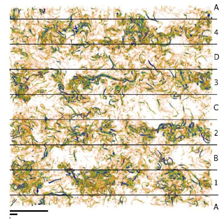
Figure 1: (Color online) Rendering of enstrophy density in a $1024\times 64\times 1024$ slice of Run III. Bands of strong (1,2,3,4) and weak (A,B,C,D) shear in the external Taylor-Green force are indicated. The bars at the bottom show respectively the integral, Taylor, and dissipation scales.

Run III is a $1024^{3}$ simulation using TG forcing. After reaching a turbulent steady state, the simulation was continued for 10 turnover times. The expression of the forcing has several spatial symmetries, and some of these symmetries are recovered in the flow in a statistical sense. Figure 1 shows a rendering of enstrophy density in a thin slice of $1024\times 64\times 1024$ grid points. Thin and elongated structures (vortex tubes) can be identified. As observed in previous studies, these structures are characterized by one large lengthscale in one direction (ranging from the Taylor to the integral scale) and a short lengthscale (close to the viscous dissipation scale) in the other two directions.

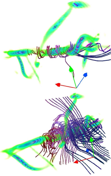
Figure 2: (Color online) Zoom on a region with large enstrophy density showing field lines inside (above) and in its surrounding (below) in Run III. Velocity field lines are helical inside and in the vicinity of the tube. Note the merging of two tubes in the south west corner. The side of the region shown is approximately one tenth of the side of the total domain.

Since $k_{F}=2$, there are four planes in the $z$ direction where the external force is zero (see Eq. 7) and the shear is maximum. In the steady state turbulent flow, these planes can be easily recognized since four bands where the vorticity is stronger are formed around them. Regions with less (or weaker) vortex tubes separate these planes, regions centered around the planes where the large scale shear has a minimum. Together, these two sets of regions form a large scale pattern that is observed to persist for long times, giving four “quiet” stripes and four stripes of “stronger” turbulence (the boundary between these regions is not well defined and fluctuates in space and time, see Fig. 1). Considering the persistence of these statistical symmetries of the flow, the velocity increments for this Run will be computed for displacements only in the $x$-$y$ plane.

Figure 3: Energy spectrum compensated by $k^{-5/3}$ for Run III. The inset shows the energy flux.

When individual vortex tubes are studied, it is seen that the flow inside and surrounding the vortex tube is helical, as noted before by several authors Tsinober and Levich (1983); Moffatt (1985, 1986); Levich (1987); Farge et al. (2001). Figure 2 shows a rendering of a small region in the domain (approximately one tenth of the box). A region of large enstrophy density is indicated by dark (blue) colors, and field lines inside and in the vicinity of the enstrophy containing region are shown. In this region and its surroundings, field lines are helical, while the flow far from the region is not. This feature has been verified for a large set of vortex tubes in the complete domain. It has been claimed in the past Moffatt and Tsinober (1992); Tsinober (2001) that the development of these helical structures in a turbulent flow can lead to the depletion of nonlinearity and a quenching of local interactions. We will come back to this issue in the following sections.

Figure 4: Probability density functions of transverse velocity increments for Run III, for increments $l=20\eta$ ($\cdots$), $l=10\eta$ ($---$), $l=4\eta$ ($-\cdot-$), $l=2\eta$ ($-\cdots-$), and $l=\eta$ (solid line), where $\eta$ is the Kolmogorov dissipation scale.

In spite of the presence of the large scale pattern, many features often associated with isotropic and homogeneous turbulence can be observed in this simulation. Figure 3 shows the angle-averaged Fourier energy spectrum and energy flux. An inertial range with constant energy flux is observed, together with a Kolmogorov-like scaling and a bottleneck as the dissipative range is reached. When probability density functions (pdfs) of transverse velocity increments

$$\delta v_{\perp}({\bf x},l)=\hat{\bf r}\times\left[{\bf v}({\bf x}+l\hat{\bf r})-{\bf v}({\bf x})\right],$$ (21)

are computed in the whole domain (Fig. 4), we observe distributions close to Gaussian for large increments, and the development of exponential and stretched exponential tails as the increment $l$ is decreased.

Figure 5: Probability density functions of transverse velocity increments with $l=10\eta$ for Run III. The solid line corresponds to the whole domain, dashed lines to regions 1 to 4 (strong shear), and dotted lines to regions A to D (weak shear; see Fig. 1). Notice the weak but systematic differences: the four dashed lines (some of them overlapping) have slower decaying tails and the dotted lines have faster decaying tails.

Figure 6: Probability density functions of transverse velocity increments with $l=2\eta$ for Run III. Same labels as in Fig. 5. Note that the differences between quiet and strong regions appear even more systematic at this scale than in Fig. 5.

Figures 5 and 6 show pdfs of transverse velocity increments with $l=10\eta$ and $2\eta$ respectively, but discriminating between bands of strong and weak shear (as indicated in Fig. 1). Bands with strong shear (1,2,3, and 4) have slightly but systematically stronger tails (i.e. a larger probability of strong gradients) than regions A,B,C, and D. Note this behavior is true for each individual region, and the difference increases as the increment $l$ is decreased. This confirms statistically what can be inferred from Fig. 1: regions of strong shear have a larger density of vortex tubes and stronger gradients.

Figure 7: First order structure function $S_{1}(l)$ for Run III. The solid line corresponds to the whole domain, dashed lines to regions 1,2,3, and 4, and dotted lines to regions A,B,C, and D. The Kolmogorov scaling and the linear slope corresponding to a smooth flow are shown as a reference. The arrow indicates the Kolmogorov scale $\eta$. Notice again the systematic differences between the two regimes identified in Fig. 1.

Figure 8: Second order structure function $S_{2}(l)$ for Run III. Labels are as in Fig. 7.

We can also compute longitudinal velocity increments

$$\delta v_{\parallel}({\bf x},l)=\hat{\bf r}\cdot\left[{\bf v}({\bf x}+l\hat{\bf r})-{\bf v}({\bf x})\right].$$ (22)

Figures 7 and 8 show respectively the second and third order longitudinal structure functions, where the structure function of order $p$ is defined as

$$S_{p}(l)=\left<\delta v_{\parallel}^{p}({\bf x},l)\right>.$$ (23)

At scales smaller than the dissipation scale the field is smooth and the structure function of order $p$ scales as $l^{p}$. Kolmogorov’s 1941 theory of turbulence predicts in the inertial range a scaling $S_{p}(l)\sim l^{p/3}$, although corrections due to intermittency are known and in general $S_{p}(l)\sim l^{\zeta_{p}}$, where $\zeta_{p}\not=p/3$ are the scaling exponents.

As with pdfs of velocity increments, a clear trend separating regions of strong and weak shear is observed. In the range of scales corresponding to the inertial range, the four regions with strong shear (regions 1,2,3 and 4) show a larger slope than the four regions with weak shear. The slope of the structure function computed in the whole box lies between these two values. Considering the results from both pdfs and structure functions, a correlation is observed between small scale gradients and large scale shear. Note that a correlation between stronger tails in the pdfs of velocity increments and vortex tubes has already been observed in Levi and Montgomery (2001); Farge et al. (2001). Here, a correlation between these quantities with large scale shear is further observed, in agreement with Ref. Laval et al. (2001) that suggests intermittency is related with interactions with the large scale flow.

III.2 Interactions, energy transfer, and flux

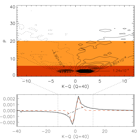
Figure 9: (Color online) Above: amplitude of triadic interactions as given by $T_{3}(K,P,Q)$ at $Q=40$ for Run III. Solid lines correspond to positive contour levels, and dotted lines to negative values. The dark (red) shaded region indicates shells in $P$ close to the forcing shell, while the light (orange) shaded region indicates shells in $P$ outside the local octave. Below: total shell-to-shell energy transfer $T_{2}(K,Q)$, transfer $T_{2}^{\textrm{L}S}(K,Q)$ due to interactions with $P$ close to the forcing shell (dashed line), and difference between these two transfers (dash-dotted line).

Figure 9 shows the functions $T_{3}(K,P,Q)$ and $T_{2}(K,Q)$ evaluated at $Q=40$ in the turbulent steady state of Run III. When triadic interactions between shells are studied, the strongest interactions are with the shell $P=3$, where the large scale forcing is. Local interactions between Fourier shells ($K\sim P\sim Q$) are two orders of magnitude smaller than nonlocal interactions with $P\sim k_{F}$. As a result, when $T_{3}(K,P,Q)$ is summed over all $P$ to obtain the shell-to-shell energy transfer $T_{2}(K,Q)$, the energy is observed to be transfered to small scales locally between shells, but with a step proportional to $k_{F}$. In $T_{2}(K,Q)$, the negative peak at $K\sim Q-k_{F}$ means energy is transfered from this shell to the shell $Q$, while the positive peak at $K\sim Q+k_{F}$ indicates energy is transfered to this shell from the shell $Q$.

The function $T_{3}(K,P,Q)$ was studied in the steady state of this run also for $Q=10$ and $Q=20$, obtaining the same quantitative results: a dominance (when compared in amplitude) of triadic interactions with the large scale flow over local triadic interactions. The $T_{2}(K,Q)$ function for all values of $Q$ between $10$ and $80$ also peaks at $K\approx Q\pm k_{F}$ (see Ref. Alexakis et al. (2005a)). These peaks at fixed values of $K-Q$ in $T_{2}(K,Q)$ are just the signature of the strong triadic interactions with the large scale forcing. If we compute the shell-to-shell transfer between shells $K$ and $Q$ due only to interactions with the large scale flow

$$T_{2}^{\textrm{L}S}(K,Q)=\sum_{P=0}^{6}T_{3}(K,P,Q)\,,$$ (24)

we obtain most of the shell-to-shell transfer (see Fig. 9). The remaining transfer $T_{2}(K,Q)-T_{2}^{\textrm{L}S}(K,Q)$ still peaks at larger wavenumbers, although it still does not peak at $K\sim Q=40$. This is due to nonlocal interactions outside the octave band not related with the large scale forcing (light shaded region in Fig. 9). Note that the definition of the range summed over $P$ in Eq. (24), or of octave bands (here defined as $Q/2\lesssim K\lesssim 2Q$) is somewhat arbitrary.

Figure 10: Total energy flux $\Pi(k)$ in Run III (solid line), flux $\Pi^{\textrm{L}S}(k)$ due to interactions with the large scale flow (dashed line), and nonlocal flux $\Pi^{\textrm{N}L}(k)$.

As previously mentioned, while individual triadic interactions as described by $T_{3}(K,P,Q)$ are dominantly nonlocal, the shell-to-shell transfer $T_{2}(K,P,Q)$ describes a local transfer of energy although through interactions with the large scale flow. Clearly when we sum over shells, the larger number of modes in the small scales start dominating over the large scale modes. Summing further over $K$ and $Q$, from Eq. (13) we can obtain the total energy flux. In analogy with Eq. (24) we can also define the flux due to interactions with the large scale flow (dark shaded region in Fig. 9)

$$\Pi^{\textrm{L}S}(k)=\sum_{P=0}^{6}\Pi_{P}(k)\,,$$ (25)

and the nonlocal flux due to interactions outside an octave band (light shaded regions in Fig. 9)

$$\Pi^{\textrm{N}L}(k)=\sum_{P=7}^{k/2}\Pi_{P}(k)\,,$$ (26)

where $\Pi_{P}(k)$ is defined in Eq. (15).

Figure 10 shows these three fluxes in the steady state of Run III. The large scale flow is only responsible for a small (but not insignificant) fraction of the total energy flux ($\Pi^{\textrm{L}S}\simeq 0.2\Pi$). Furthermore although the amplitude of the nonlocal flux $\Pi^{\textrm{N}L}(k)$ depends on the definition of an octave band, it is remarkable that it peaks at wavenumbers close to the peak of the bottleneck in the energy spectrum (see Fig. 3). This gives a direct confirmation that the bottleneck is due to the depletion of the energy transfer due to local interactions with $K\sim P\sim Q$. These interactions are inhibited because of the presence of a numerical and/or viscous cutoff in wavenumber, and nonlocal triads become dominant Herring et al. (1982); Falkovich (1994); Lohse and Müller-Groeling (1995); Martínez et al. (1997). Indeed, in Ref. Herring et al. (1982) it was shown using the eddy-damped quasinormal Markovian (EDQNM) approximation that the bottleneck disappears if nonlocal interactions are excluded from the computation. Note that the spurious drop of the fluxes $\Pi^{\textrm{L}S}$ and $\Pi^{\textrm{N}L}$ at $k=80$ in Fig. 10 is because the functions $T_{3}(Q,P,Q)$ and $T_{2}(K,Q)$ were only computed up to this wavenumber.

Therefore there seems to be a hierarchy concerning the importance of nonlocality when one investigates the transfer functions. At the most basic level when one investigates the transfer function $T_{3}$ the interactions with the large scale flow are the strongest ones. When averaged over the middle wave number the resulting energy transfer $T_{2}$ becomes local but not self-similar with a maximum at $K-Q\sim k_{F}$. When averaged further to obtain the energy flux, the non local interactions with the large scale flow are only responsible for 20% of the flux.

IV Scaling with Reynolds

In this section we discuss results from runs I, II, and III. The three runs are forced using Eq. (7), and the only parameters changed between the runs are the spatial resolution and the kinematic viscosity. This investigation allows us to study how the results about the non-local interactions change as we increase the Reynolds number. Qualitatively the functions $T_{3}(K,P,Q)$ and $T_{2}(K,Q)$ are similar for all three runs: the strongest interactions [$T_{3}(K,P,Q)$] are with the large scale flow and the energy transfer [$T_{2}(K,Q)$] is local with the two peaks at $K-Q\sim k_{F}$. For this reason we focus here on the study of the local and nonlocal flux of energy as the Reynolds number is changed.

Figure 11: Scale variation of the flux ratio $\Pi^{\textrm{L}S}/\Pi$ for increasing Reynolds numbers; Runs I (dash-dot line), II (dash line), and III (solid line). Note the presence of a wavenumber range where $\Pi^{\textrm{L}S}/\Pi$ becomes constant only for the highest resolution run.

In Figure 11 we show the ratio of the flux $\Pi^{\textrm{L}S}(k)$ to the total flux $\Pi(k)$. As discussed in the previous section, the flux due to interactions with the large flow gets diminished as we sum over more and more modes. As a result, in the inertial range of Run III interactions with the large scale flow are only responsible for $\sim 20\%$ of the energy flux. In the smaller Reynolds number runs (I and II), the amount of flux due to interactions with the large scale flow is larger. This implies that as we increase the Reynolds number the fraction of the energy flux in the inertial range due to interactions with the large scale flow decreases. However, note that in Run III a region in the inertial range where the ratio $\Pi^{\textrm{L}S}/\Pi$ is approximately constant is observed. This region with constant ratio $\Pi^{\textrm{L}S}/\Pi$ is not present in the simulations with lower Reynolds number. Therefore DNS with even higher Reynolds number than what is accomplished here are needed to determine how does this ratio scale with the Reynolds number.

V Effects of different forcing functions

V.1 Forcing expression and correlation time

Figure 12: Compensated energy spectrum $k^{5/3}E(k)$ (solid line) and helicity spectrum $k^{5/3}H(k)/k_{F}$ (dashed line) in the steady state of Run VII, where $k_{F}$ is the forcing wavenumber.

Nonlocal interactions discussed in the previous section were observed for runs with large scale non-helical forcing with infinite correlation time. It is of interest to know how much of these results translate to other kind of forcings. In this section we compare results for runs III, VII and VIII. Run VII is a $1024^{3}$ simulation with constant helical forcing, and as runs I-III, it also displays a well defined large scale flow (for a description of the ABC flow, see e.g. Ref. Childress and Gilbert (1995)). In Run VIII the phases of the forcing function are changed randomly with a short correlation time. Although the resolution in this run is smaller ($256^{3}$), we will focus here on the effect of the forcing, since a systematic study of changing the Reynolds number for fixed forcing was presented in the previous section.

Figure 12 shows the energy and helicity spectra compensated by a Kolmogorov law in the turbulent steady state of Run VII. As proposed in Ref. Brissaud et al. (1973) and observed in several simulations André and Lesieur (1997); Borue and Orszag (1997); Chen et al. (2003a, b); Gómez and Mininni (2004) the spectrum of helicity follows a Kolmogorov law and is proportional to $k_{F}E(k)$. The transfer of helicity will be discussed in Section VI.

Figure 13: Scaling exponents of velocity structure functions $\zeta_{p}$ as a function of order $p$ in Runs III (TG forcing) and VII (ABC forcing). The Kolmogorov K41 scaling Kolmogorov (1941) is indicated, as well as the She-Leveque (SL) prediction She and Lévêque (1994). Note the difference between TG and ABC.

Figure 13 shows the scaling exponents $\zeta_{p}$ of the longitudinal structure functions, computed for runs III and VII. The extended self-similarity (ESS) hypothesis Benzi et al. (1993a, b) was used to compute the anomalous exponents, which show similar behavior for both runs. However, the resulting exponents for $p>3$ from Run VII (ABC forcing) are slightly smaller than the exponents from Run III (TG forcing); for example, in Run III $\zeta_{4}=1.2737\pm 0.0005$ and $\zeta_{8}=2.136\pm 0.006$, while in Run VII $\zeta_{4}=1.2647\pm 0.0005$ and $\zeta_{8}=2.026\pm 0.008$. Note that the difference between the scaling exponents for TG and ABC at order $p=4$, though small, is nevertheless more than order of magnitude larger than the error arising from measuring them by virtue of the ESS hypothesis which leads to negligible errors.

It should be noted that it is unclear whether this observed difference is due to problems linked with using the ESS methodology itself, or if it indicates a departure from universality between these two flows because of loss of homogeneity, as exemplified in Fig. 1. Since the two forcing functions studied here are both to some degree anisotropic and inhomogeneous, subleading contributions due to departures from full symmetry could be responsible for this discrepancy. In this context, a decomposition of the structure functions into their isotropic and anisotropic components Biferale and Toschi (2001); Biferale and Vergassola (2001); Biferale et al. (2002) could help to asses the degree of universality of each component. These points will necessitate further study and better resolved flows.

Figure 14: Shell-to-shell energy transfer function $T_{2}(K,Q)$ for Run VII. The superimposed curves correspond to different values of $Q$, with $Q\in[10,80]$.

The shell-to-shell energy transfer $T_{2}(K,Q)$ for Run VII is shown in Fig. 14. As for non-helical forcing (see Sec. III and Ref. Alexakis et al. (2005b)) the shell-to-shell transfer function peaks at $K\approx Q\pm k_{F}$, indicating the transfer of energy is local but mediated by nonlocal interactions with the large scales. If we sum over $K$ and $Q$ to obtain the energy flux, we reobtain the results discussed in Sec. IV for Run III: most of the energy flux is local, although in the inertial range $\sim 20\%$ of the total flux is due to interactions with the large scale forcing.

The transfer function $T_{2}(K,Q)$ was also computed in the turbulent steady state of Run VIII (see Fig. 15.a). In this run the phases of the external force are changed randomly with a short correlation time. It is noteworthy that even in this case with isotropic and random forcing, evidence is found of nonlocal interactions with the large forcing scale: the $T_{2}(K,Q)$ function peaks at $K\approx Q\pm k_{F}$ for all wavenumbers $Q$ studied (note that in this run $k_{F}=1$). Fig. 15 is discussed further below.

V.2 Forcing scale

Figure 15: Shell-to-shell energy transfer function $T_{2}(K,Q)$ for runs with different forcing wavenumbers $k_{F}$ as indicated by the vertical lines; Run VIII with $k_{F}=1$ (a), Run V with $k_{F}=3$ (b), and Run IV with $k_{F}=10$ (c). In each panel, the several curves correspond to different values of $Q$ in the inertial and dissipative ranges. Note that for each run, the peak of energy transfer is centered close to $k_{F}$.

Through all this work we have shown transfer functions indicating that the energy is locally transfered between scales but with a fixed step that we associated with the forcing scale. In this subsection we compare the transfer function $T_{2}(K,Q)$ in simulations forced at different wavenumbers.

Figure 15 shows $T_{2}(K,Q)$ for several values of $Q$ computed in the steady state of runs VIII ($k_{F}=1$), IV ($k_{F}=2$), and V ($k_{F}=10$). A clear correlation is observed between the position of the peaks ($|K-Q|$) in the shell-to-shell transfer function, and the forcing wavenumber $k_{F}$. In the last case, the peaks at $|K-Q|$ slightly smaller than $k_{F}$ could be associated with low Reynolds number effects.

VI Helicity transfer

The transfer of helicity is readily studied in Run VII, since the external forcing injects maximum helicity and all scales are dominated by the same sign of helicity. We will make no attempt here to separate the different signs of helicity in the simulations (see e.g. Refs. Waleffe (1991); Chen et al. (2003a, b)).

Figure 16: The spectrum of relative helicity $H(k)/kE(k)$ compensated by $k^{-1}$ for run VII. Note that the region where the spectrum is flat indicates a power law of $k^{-1}$ in the relative helicity. At large wavenumber, a $k^{1/2}$ slope is shown only as a reference. The increase at large $k$ is indicative of an excess of relative helicity in the small scales.

Before discussing the transfer of helicity, it is of interest to study spectral properties of helical flows. As previously discussed, the spectrum of helicity follows an approximate $k^{-5/3}$ law (see Fig. 12). As a result, the relative helicity $H(k)/E(k)k$ follows in the inertial range a $k^{-1}$ slope Brissaud et al. (1973); André and Lesieur (1997); Lesieur (1997) (i.e. small scales are less helical than large scales). It was predicted in Refs. Ditlevsen and Giuliani (2001a, b) that the dissipation scale of helicity should be larger than the energy dissipation scale, giving as a result a drop in the spectrum of relative helicity faster than $k^{-1}$ for small scales. This argument would be in agreement with the idea that small scales slowly recover the mirror symmetry broken by the injection of helicity in the large scales. However, previous simulations Gómez and Mininni (2004) and this high resolution run both suggest that there is an excess of relative helicity in the small scales, when compared with the $k^{-1}$ drop. Note that this slower than predicted recovery of symmetries in the small scales is also in agreement with the slower than expected recovery of isotropy observed in experiments Sreenivasan and Antonia (1997); Shen and Warhaft (2000).

Figure 16 shows $H(k)/E(k)$, i.e. the spectrum of relative helicity $R(k)=H(k)/kE(k)$ compensated by $k^{-1}$. A scaling of $k^{-1}$ for the relative helicity $R(k)$ thus corresponds to a flat spectrum in Fig. 16, as observed through the inertial range up to $k\sim 20$. However, at small scales the compensated spectrum of relative helicity grows, possibly as $k^{1/2}$ or steeper, indicating that the spectrum of helicity $H(k)$ at small scales is dropping slower than the spectrum of energy $E(k)$ (see also Fig. 12). This can be associated with the presence of vortex tubes, that are known to be helical (see Fig. 2).

Figure 17: Energy spectrum compensated by $k^{-5/3}$ for Runs V (dashed line), VI (dotted line), and VII (solid line). All runs are for ABC forcing at different Reynolds numbers. Note the wavenumber on the x-axis has been divided by the dissipation wavenumber to make all dissipation ranges coincide. A slope of $1/3$ close to the bottleneck (corresponding to a power law of $k^{-4/3}$ in the energy spectrum) is shown as a reference.

The effect of helicity, and indirectly the effect of nonlocal interactions which can be modeled for example through the introduction of a second time-scale in the problem in order to distinguish between the eddy turn-over time and a helical characteristic time, has also been used to explain the development of the bottleneck effect that occurs at the onset of the dissipative range, see e.g. Kurien et al. (2004). Ref. Kurien et al. (2004) predicts a $k^{-4/3}$ energy spectrum for the bottleneck, that we found compatible with our spectra for runs V-VII (Fig. 17). We also observe a $k^{-4/3}$ range close to the bottleneck in the Taylor-Green flow that has no net helicity. Note that the argument in Ref. Kurien et al. (2004) is based on the presence of non zero helicity locally. The transition from the inertial range to the bottleneck seems to be dependent on the Reynolds number. It is worth noting that while at resolutions of $256^{3}$ mostly a bottleneck is observed, in the $1024^{3}$ runs a short Kolmogorov-like scaling is found before the bottleneck takes place. The origin of the bottleneck based on the dominance of nonlocal interactions in the dissipative range has also been investigated Herring et al. (1982); Falkovich (1994); Lohse and Müller-Groeling (1995); Martínez et al. (1997) as we discussed in Sec. III, and is independent of the presence of helicity. These arguments are not mutually exclusive, as local in space generation of helicity in the small scales can also quench local interactions between eddies of comparable sizes. However, the prediction in Ref. Falkovich (1994) for the spectral shape of the bottleneck is in disagreement with the spectra obtained in all simulations here. These points deserve further study at higher resolution if one is to be able to distinguish between the different ranges that may be occurring.

Figure 18: Shell-to-shell helicity transfer $T_{H}(K,Q)$ in Run VII, for all values of $Q$ from $10$ to $80$.

Finally, we discuss the shell-to-shell helicity transfer $T_{H}(K,Q)$ in Run VII (Fig. 18). As for the transfer of energy, the helical transfer function peaks at $K\approx Q\pm k_{F}$, although this transfer is noisier. The helicity cascades directly to smaller scales as the energy, confirming previous studies Borue and Orszag (1997); Chen et al. (2003a, b); Gómez and Mininni (2004). The helicity is not a positive definite quantity, and as a result both signs of the transfer can indicate a direct cascade depending on the sign of the helicity itself. Moreover, as we study smaller scales and the relative helicity decreases, both signs have more predominance increasing the noise observed in $T_{H}(K,Q)$.

VII Conclusions

We start by summarizing our results. The energy transfer, triadic interactions, and statistical flow properties were studied in several high resolution DNS with periodic boundaries. The spatial resolution ranged from $256^{3}$ to $1024^{3}$. The Reynolds number based on the integral scale spanned values from $R_{e}\approx 275$ to $6200$, while the Taylor-based Reynolds number varied between $R_{\lambda}\approx 230$ and $1100$. Three forcing functions were used, two coherent functions with zero and maximum net helicity respectively, and a random forcing with a short correlation time. The energy injection scale was also varied to study its impact on the energy transfer.

Most statistical studies were done for Run III, a high resolution simulation with $R_{\lambda}\approx 800$ and TG forcing. The forcing and the resulting flow have spatial symmetries that allow us to identify planes with strong and weak large scale shear easily. While in the whole domain the standard results were reobtained (e.g. exponential and stretched exponential tails in the pdfs of velocity increments, and anomalous scaling of the structure functions), when studying individual regions a correlation between large scale shear and small scale gradients was found. In regions of strong shear, the tails of the pdfs of velocity increments are stronger than in regions of weak shear, even at scales as small as twice the dissipation scale. Also, structure functions show a slightly larger slope in regions of strong large scale shear, i.e. a larger departure from a Kolmogorov $p/3$ self-similar scaling.

A correlation between stronger tails in the pdfs of velocity increments and the presence of vortex tubes has already been observed in different decompositions of the flow Levi and Montgomery (2001); Farge et al. (2001). Here, we observed a correlation between these quantities and the large scale shear. The correlation was observed to be persistent even at scales as small as the dissipation scale. Small differences were also observed in the anomalous scaling of the structure functions for TG and ABC forcing. However, it is unclear whether this is related with non-universal effects associated with interactions with the large scale forcing, or with the use of the ESS hypothesis. For individual vortex tubes in several flows, we verified that the flow inside and surrounding the vortex tube is helical, as found before Tsinober and Levich (1983); Moffatt (1985, 1986); Levich (1987); Farge et al. (2001). Note that the development of helical structures in a turbulent flow can lead to the depletion on nonlinearity and a quenching of local interactions Moffatt and Tsinober (1992); Tsinober (2001).

Concerning the energy transfer and triadic interactions, we confirmed for several forcing functions that the cascade of energy is local between Fourier shells, although it is strongly mediated by individual triadic interactions which are nonlocal in nature. As a result, the energy cascades from one shell to the next with a fixed step proportional to the forcing wavenumber $k_{F}$. This effect was observed even in simulations using random forcing with a correlation time one order of magnitude smaller than the large scale turnover time. No qualitative differences have been observed as the Reynolds number was changed.

However, the degree of nonlocality observed depends on the quantity studied. A hierarchy is found in the relative amplitude of nonlocal effects in triadic interactions, the shell-to-shell energy transfer, and the energy flux. Triadic interactions are dominated by interactions with the large scale flow. As more modes are summed to define the shell-to-shell transfer and the flux, the larger population of small scale modes starts dominating, and in the $1024^{3}$ simulations the large scale flow is responsible for only $\sim 20\%$ of the total flux.

An increase of the relative contribution of nonlocal interactions (with the large scale flow and with modes outside the octave band studied) in the total flux is observed as the dissipative range is reached. This result is in good agreement with claims that the bottleneck effect is due to the quenching of local interactions at the end of the inertial range because of the presence of a cut-off in wavenumbers Herring et al. (1982); Lohse and Müller-Groeling (1995); Martínez et al. (1997).

It is worth noting that the local energy cascade through nonlocal interactions, or non negligible nonlocal interactions, has been observed in the past in simulations at lower Reynolds numbers (see e.g. Refs. Domaradzki and Rogallo (1990); Ohkitani and Kida (1992); Yeung et al. (1995); Zhou et al. (1996)). Our results confirm the presence of interactions between disparate scales in a turbulent flow at much larger Reynolds numbers, and for a variety of forcing functions and forcing scales. The results discussed here also shed some light on the controversy in the literature about the relevance of the nonlocal interactions. It has been claimed that interactions are local if a different measure for the locality is introduced Zhou (1993a, b), or if wavelets or a binning of Fourier space in octaves is used Kishida et al. (1999) (note that wavelets naturally introduce a binning in octaves of the spectral space). The hierarchy found in the different transfer functions is the reason for this apparent inconsistency between previous results. As more modes are summed (e.g. to define octaves in spectral space, or to define our partial fluxes $\Pi_{P}$), the small scales overcome the triadic interactions with the large scale flow, and local interactions give the largest contribution. This is also in agreement with recent theoretical results about the locality of the energy flux Eyink (2005), or the locality of the shell-to-shell energy transfer in Fourier octave bands Eyink (1994); Verma et al. (2005).

The fact that in simulations with $R_{\lambda}\sim 1000$ most of the flux is due to local interactions, does not preclude however the existence of strong nonlocal interactions with the large scale flow at the triadic interaction level, and it should be kept in mind that even at large values of $R_{\lambda}$ these interactions are responsible for a non-negligible fraction of the total flux. The presence of nonlocal interactions are a deviation from the standard hypothesis often associated with Kolmogorov (K41) theory Kolmogorov (1941), and can possibly explain departures from self-similar models of the higher order structure functions and controversial results observed in experiments, such as the slower than predicted recovery of isotropy in the small scales Shen and Warhaft (2000).

Similar results were obtained for the helicity transfer. The injection of net helicity in the large scales breaks down the mirror symmetry in the flow. While confirming the direct cascade of helicity Brissaud et al. (1973); André and Lesieur (1997); Borue and Orszag (1997); Chen et al. (2003a, b); Gómez and Mininni (2004), we also found a slower than expected recovery of the symmetries in the small scales, with an excess of relative helicity at small scales compared with the $k^{-1}$ expected drop. As in the energy cascade, the cascade of helicity takes place in fixed steps proportional to the forcing scale, indicating strong nonlocal triadic interactions.

Nonlocal interactions can also be responsible for observed departures from universality. In Alexakis et al. (2005a) it was shown with a simple dimensional argument how nonlocal interactions can still be consistent with a $k^{-5/3}$ energy spectrum. Vortex tube stretching by the large scale flow plays a significant role, and the argument has points in common with multifractal models of intermittency, such as the $\beta$ model (see e.g. Frisch (1995)). As previously mentioned, in this work we showed evidence of a positive correlation of large scale shear and small scale gradients, both in pdfs of velocity increments and in structure functions. Ref. Laval et al. (2001) showed that the anomalous scaling of the structure functions is reduced when nonlocal interactions with the large scale flow are artificially suppressed in a simulation. Both results suggest that departures from K41 theory can be associated with the imprint of the large scale forcing in turbulence.

The modern language used in turbulence is related to a great extent to the K41 theory developed for the isotropic and homogeneous case, with the assumption that such fundamental symmetries of the equations would be recovered in the small scales even when broken (e.g. through external forcing) in the large scales. To apply this theory to real turbulent flows, the idea that small scales restore isotropy and homogeneity is based strongly on the assumption of local interactions between scales. The persistence of anisotropies and other deviations from K41 observed in experiments and simulations have been associated in this work with the presence of strong non-local triadic interactions. At this point, the reader could ask how much of the edifice of homogeneous and isotropic turbulence remains.

One of the assumptions in K41 theory is that the properties of the inertial range are universal. This is directly related to the assumption of local interactions. Since eddies in the inertial range only interact with eddies of similar size, as the energy cascades through the inertial range a self-similar solution is obtained. The fraction of the flux due to non-local interactions, found to be $\sim 20\%$ here, can be interpreted as a subleading contribution to the local flux. Deviations from K41 theory are well documented and several theories have been proposed to explain them (see e.g. Kolmogorov (1962); She and Lévêque (1994); Frisch (1995); Lesieur (1997); Tsinober (2001)). They have also been derived theoretically for the passive scalar in the context of the so-called Kraichnan model Kraichnan (1968). Several of these corrections were associated with viscous effects for turbulence at finite Reynolds number. What our results show is that these deviations can come as well from interactions with the large scale flow. In this context, simulations at higher resolution could help to study the scaling of the non-local flux with the Reynolds number.

It is known that in the Kraichnan model only prefactors of the scaling laws depend on the large-scale forcing (i.e. the exponents are universal: independent of the forcing). However, in the case of the Navier-Stokes equations, this has not been proved yet since the hierarchy of equations for the $n$-point correlation functions is not closed. Then, inertial range solutions with exponents that depend on the forcing may exist.

In the case of realistic turbulent flows as encountered in astrophysics and geophysics, the presence of strong non-local interactions can lead to the persistence of anisotropies in the small scales. In this case, the anisotropic effects question the applicability of the theory of isotropic and homogeneous turbulence to real flows (at least at Reynolds numbers comparable to the ones studied in this work). The properties of the large scale flow can be more important than expected to shape the small scales. A systematic study of the isotropic and anisotropic contributions to the scaling Biferale and Toschi (2001); Biferale and Vergassola (2001); Biferale et al. (2002) can be a first step to recognize universal (and non-universal) features in these cases.

Finally, as previously indicated in Alexakis et al. (2005a), the existence of non-negligible nonlocal interactions in a variety of turbulent flows gives support to models involving as an essential agent of the nonlinear energy transfer the distortion of turbulent eddies by a large-scale flow (e.g. as in rapid distortion theory and its variants Laval et al. (2001); Dubrulle et al. (2004), or as in the Lagrangian averaged Navier-Stokes equations Holm et al. (1998); Chen et al. (1998) where the turbulent flow interacts with a smooth velocity field). We believe that the understanding of scale interactions in turbulence can lead to the development of a new generation of subgrid models, beyond the usual hypothesis of locality done in most Large Eddy Simulations.