Magnetohydrodynamic activity inside a sphere

Abstract

We present a computational method to solve the magnetohydrodynamic equations in spherical geometry. The technique is fully nonlinear and wholly spectral, and uses an expansion basis that is adapted to the geometry: Chandrasekhar-Kendall vector eigenfunctions of the curl. The resulting lower spatial resolution is somewhat offset by being able to build all the boundary conditions into each of the orthogonal expansion functions and by the disappearance of any difficulties caused by singularities at the center of the sphere. The results reported here are for mechanically and magnetically isolated spheres, although different boundary conditions could be studied by adapting the same method. The intent is to be able to study the nonlinear dynamical evolution of those aspects that are peculiar to the spherical geometry at only moderate Reynolds numbers. The code is parallelized, and will preserve to high accuracy the ideal magnetohydrodynamic (MHD) invariants of the system (global energy, magnetic helicity, cross helicity). Examples of results for selective decay and mechanically-driven dynamo simulations are discussed. In the dynamo cases, spontaneous flips of the dipole orientation are observed.

I INTRODUCTION

Magnetohydrodynamic “dynamo” processes are those in which the motions of an electrically conducting fluid amplify and maintain a finite magnetic field, starting from an arbitrarily small one. They have long been of interest for geophysics and astrophysics Moffatt ; Glatzmaier95 ; Dikpati99 ; Kono02 ; Nandy02 ; Mininni04 , and have more recently become of interest with regard to laboratory attempts to generate dynamo magnetic fields in liquid metals Gailitis01 ; Steiglitz01 ; Noguchi02 ; Petrelis03 ; Sisan03 ; Spence05 . The relevant theoretical and computational literature is vast, and extensive reviews have recently been given (see e.g. Refs. Roberts01 ; Kono02 ; Brandenburg05 ).

In our own work, we have lately been studying dynamo processes numerically, using turbulent three-dimensional magnetohydrodynamic (hereafter, “MHD”) codes of the familiar Orszag-Patterson pseudospectral variety Ponty05 ; Mininni05a ; Mininni05b ; Alexakis05 ; Mininni05c . Such codes treat homogeneous turbulence efficiently, but are mainly useful in situations involving spatially periodic boundary conditions. Particularly for the case of planetary dynamos and laboratory experiments, restrictions to periodic boundary conditions are a severe limitation. Essential ingredients, such as rotation, global angular momentum, and the interfaces between conducting and non-conducting regions are not readily included. It is to be expected that all of these play a role in the physical situations of interest, and give rise to qualitatively new physical processes not accessible with periodic boundaries.

This present paper represents our attempt to begin a study of these processes by introducing, and displaying some results from, a computational method that is adapted to the geometry of isolated spheres. Our goal is not to reach realistic geophysical parameter regimes (out of the question for the foreseeable future, in any case), but rather to isolate and study those new physical processes that appear in this geometrically more realistic setting. Our results are not to be compared with the ambitious geo-dynamo computation of Glatzmaier and Roberts (e.g., Refs. [2,21]) who include far more physical effects and degrees of freedom than we have at this point. We will consider it not to be a limitation on our work if we are unable to reach realistic Reynolds numbers, so long as the spectra of the dynamo processes we do identify are well-resolved by the number of expansion functions we are able to retain. We think of these efforts as studies of dynamo behaviors exhibited by the MHD equations in spherical geometry without regard to their present applicability to geophysical or laboratory situations. It appears not to be necessary to reach presently-existing ranges of Reynolds numbers or magnetic Prandtl numbers in order to see interesting spontaneously-generated magnetic field behavior.

The numerical technique is entirely spectral, using an expansion basis that is specifically adapted to spherical geometry: the Chandrasekhar-Kendall (hereafter, “C-K”) vector eigenfunctions of the curl Chandrasekhar57 ; Turner83 ; Yoshida91 ; Yoshida92 ; Cantarella00 (by construction, C-K functions are also eigenfunctions of the Helmholtz wave equation; see e.g. Mueller ). These functions form a complete orthogonal set under the boundary conditions we will choose. They can be normalized. Their completeness has been shown by Yoshida for the cylinder Yoshida92 and by Cantarella et al Cantarella00 for the sphere. The cylindrical version was used some years ago for studying processes believed to be involved in the disruptions of fusion confinement devices Montgomery78 ; Shan91 ; Shan93a ; Shan93b ; Shan94 . Their advantages lie in their natural geometrical relation to the specific geometries in which they are employed (all the boundary conditions can be built into each expansion function) and in certain desirable numerical properties, which include the following. The MHD equations involve several solenoidal fields of which several curls are taken. Taking the curl of a C-K function simply gives the function back again, times a multiplicative constant. This means that no numerical spatial differentiations are required, with their attendant complication of the expressions and loss of accuracy. The code preserves the ideal MHD invariants very accurately over long times (total energy, magnetic helicity, cross helicity), which is one of the few accuracy checks available to a strongly nonlinear code for which non-trivial analytical solutions are scarce. In addition, the ideal invariants are readily exhibited as simple algebraic quadratic sums involving the expansion coefficients, so no numerical integrations are required to evaluate them. Going along with these advantages is a severe disadvantage associated with the lack of a fast transform for the spherical Bessel functions involved, which means that the nonlinear terms lead to convolution sums which grow rapidly with the number of expansion functions retained in the Galerkin approximation. This limits us to mechanical and magnetic Reynolds numbers of the order of a very few thousand, and makes it unlikely that we can ever reach planetary parameters without modeling the small scales of the fluid motions.

But the absence of any coordinate singularities (e.g., $r=0$ in spherical polar coordinates) to worry about anywhere is a considerable advantage, as we noted previously in solving the two-dimensional Navier-Stokes equation inside a circle with non-ideal boundaries Li96a ; Li97 . The code also can be readily parallelized and there are no potential aliasing problems.

The situation we wish to study is that of an electrically conducting fluid inside a rigid spherical boundary that isolates the fluid, mechanically and magnetically, from everything outside it. The boundary is regarded as a spherical shell that is perfectly conducting (so magnetic fields cannot penetrate the region outside) and is coated on the inside with a thin layer of insulating dielectric so that the electrical current density cannot penetrate the shell. The shell is regarded as mechanically impenetrable, so that the normal component of the fluid velocity vanishes there. We do not employ no-slip boundary conditions on the velocity field, but rather choose the vanishing of the normal component of the vorticity at the spherical boundary as the second boundary condition on the velocity field. This condition is implied by, but does not imply, no-slip boundary conditions on the velocity field, and thereby avoids certain mathematical procedures that sometimes attend the attempts at imposing no-slip boundary conditions. These four boundary conditions for the fields in the external walls, plus regularity of each component of the velocity and magnetic fields at the origin, might be thought of as a total of ten boundary conditions for the system. The above mentioned boundary condition for the vorticity in the wall is easy to implement in the present formulation. Other boundary conditions (e.g. no-slip boundary conditions) can be studied with our method using a penalty method close to the walls (as done for example in Ref. Shan94 ) and will be considered in the future. However, we want to point out that the present election of boundary conditions also avoids some problems present in hydrodynamic incompressible flows when no-slip conditions are imposed (see e.g. Kress00 ; Gallavotti for a detailed discussion). Since this topic is beyond the aim of our present study, we will use in the following these simple boundary conditions and leave the study of other options for future work.

An outline of the paper follows. Section II introduces the expansion basis and shows how the nonlinear partial differential equations can be reduced to a set of ordinary differential equations, first order in the time, for the expansion coefficients. We include mention of other possible boundary conditions that it is intended to introduce in the future, then settle on the one just described for these runs. The numerical method is discussed in Section III. Sections IV and V display our first applications of the code to some simple MHD problems that are considered interesting and that are peculiar to spherical geometry. We simultaneously explore the possibilities for some relative new flow visualization diagnostics when exhibiting our results vapor ; these are described when they appear. Section VI summarizes the results and discusses possible future applications of the method.

II THE SPECTRAL DECOMPOSITION

C-K functions are constructed from a solution of the scalar Helmholtz equation:

$$\left(\nabla^{2}+\lambda^{2}\right)\psi=0,$$ (1)

where we are referring to spherical polar coordinates $(r,\theta,\phi)$ and $\lambda$ is an eigenvalue that will eventually be determined by boundary conditions. Vector eigenfunctions of the curl appropriate to spherical geometry may be constructed according to the following recipe from each solution to Eq. (1):

$${\bf J}=\lambda\nabla\times{\bf r}\psi+\nabla\times\left(\nabla\times{\bf r}\psi\right).$$ (2)

From this, it may readily be verified that $\nabla\times{\bf J}=\lambda{\bf J}$. Thus any single ${\bf J}$ is a “force-free” or “Bernoulli” field, though the sum of two or more of them is not. The relevant scalar $\psi$ is

$$\psi_{qlm}=C_{ql}\,j_{l}(|\lambda_{ql}|r)Y_{lm}(\theta,\phi).$$ (3)

Here, $C_{ql}$ is a normalization constant, $j_{l}$ is a spherical Bessel function of order $l$, and $Y_{lm}$ is the normalized spherical harmonic expressed in terms of the polar angle $\theta$ and the azimuthal (longitudinal) angle $\phi$. The number $C_{ql}$ is chosen to make the volume integral of ${\bf J}_{qlm}\cdot{\bf J}_{qlm}^{*}$ over the computational domain equal to unity (the asterisk denotes complex conjugate).

The integer $l$ is $1,2,3,\dots$ and $m$ runs in integer steps from $-l$ to $l$. An infinite sequence of values of $\lambda_{ql}$, labeled by $q=1,2,3,\dots$ and $q=-1,-2,-3,\dots$ will be determined by a radial boundary condition momentarily to be invoked on ${\bf J}$ for a given $l$.

The boundary conditions that will be invoked, consistently with the physical description of the region and its boundaries that were given in Sec. I refer to the magnetic field ${\bf B}$ and the velocity field ${\bf v}$, both solenoidal, and their curls. The curl of ${\bf v}$ is $\omega$, the vorticity, and the curl of ${\bf B}$ is ${\bf j}$, the electric current density, in the dimensionless units that remain to be described. We shall demand that the normal (radial) components of all four vector fields vanish at the boundary $r=R$. Since these four fields are to be expanded in the ${\bf J}$’s, making the radial component of each ${\bf J}$ vanish at $r=R$ will guarantee that the boundary conditions will be satisfied for any superposition of them. This vanishing of the normal components of the ${\bf J}$ determines the allowed values of $\lambda_{ql}$, positive and negative, by the locations of the zeros of the spherical Bessel functions. Then the explicit expression for the normalization constant $C_{ql}$ is

$$C_{ql}=\left|\lambda_{ql}\,j_{l+1}(|\lambda_{ql}|R)\right|^{-1}\left[l(l+1)R^{3}\right]^{-1/2}.$$ (4)

Positive or negative $q$ is to be associated with positive or negative $\lambda_{ql}$ according to $\lambda_{-q,l}=-\lambda_{ql}$. For a variety of radial boundary conditions, including the one just chosen, the ${\bf J}_{qlm}$ functions corresponding to differing indices $q$, $l$, or $m$ can be shown to be orthogonal. Boundary conditions at two different radii can be imposed if spherical Neumann functions are also permitted in $\psi$.

Given the completeness of the C-K functions so defined, they are then appropriate for expanding various vector fields of incompressible MHD: the magnetic field, fluid velocity, vorticity, electric current density, and vector potential in the Coulomb gauge. These are considered to be the necessary set of quantities to be expanded when studying spherical MHD and dynamos in the class of problems studied here. The ones of slowest spatial variation (smaller $|q|$, low $l$ and $|m|$) contain the dipole and low-order multipole components of the fields and provide a natural ordering of the spectral contributions from various spatial scales, starting with those of the largest scales.

The MHD equations to be solved are, in familiar dimensionless (“Alfvénic”) units, common in MHD turbulence theory, an equation of motion for the fluid velocity ${\bf v}$,

$$\frac{\partial{\bf v}}{\partial t}={\bf v}\times\mbox{\boldmath$\omega$}+{\bf j}\times{\bf B}-\nabla\left({\mathcal{P}}+\frac{v^{2}}{2}\right)+\nu\nabla^{2}{\bf v}+{\bf f},$$ (5)

and the induction equation for advancing the magnetic field ${\bf B}$,

$$\frac{\partial{\bf B}}{\partial t}=\nabla\times\left({\bf v}\times{\bf B}\right)+\eta\nabla^{2}{\bf B},$$ (6)

In these units, ${\bf v}$ may be considered to be normalized by the rms value of the velocity field ($U$, say), and the magnetic field in units that, using the square root of the mass density, converts a magnetic field to an Alfvén speed based upon the same rms velocity. In Eqs. (5) and (6), lengths are measured in units of the spherical radius $R$ (the radius $R$ will be 1 in the dimensionless units) and times in units of $R/U$. ${\mathcal{P}}$ is the dimensionless ratio of pressure to mass density, with the mass density assumed to be spatially uniform. A forcing function ${\bf f}$ has been written on the right hand side of Eq. (5) to represent any externally applied mechanical force that can be chosen to mimic a variety of physical effects, a common convention in dynamo-motivated computations in periodic boundary conditions. Both ${\bf B}$ and ${\bf v}$ and their curls are solenoidal. Note that in the incompressible case, nonlinear coupling between modes is provided by the nonlinearities in both the equation of motion and the induction equation. Here, we are keeping all of these. In the context of planetary dynamos, other physical effects sometimes justify dropping the advection term in the equation of motion. Then other numerical methods (see e.g. Ref. Ivers03 ) for linearised MHD can be used.

An evolution equation for vorticity can be obtained by taking the curl of Eq. (5):

$$\frac{\partial\mbox{\boldmath$\omega$}}{\partial t}=\nabla\times\left({\bf v}\times\mbox{\boldmath$\omega$}\right)+\nabla\times\left({\bf j}\times{\bf B}\right)+\nu\nabla^{2}\mbox{\boldmath$\omega$}+\nabla\times{\bf f}.$$ (7)

Given the appropriate boundary conditions, the vorticity $\omega$ can be used to determine the velocity ${\bf v}$. The dimensionless viscosity $\nu$ and magnetic diffusivity $\eta$ can be interpreted, respectively, as reciprocals of kinetic and magnetic Reynolds numbers based on $U$, $R$, and the laboratory (dimensional) values of kinematic viscosity and magnetic diffusivity.

The numerical scheme is to solve Eqs. (5) or (7) and (6) by representing ${\bf v}$ and ${\bf B}$ as the Galerkin expansions,

$${\bf v}({\bf r},t) = \sum_{qlm}\frac{\xi^{v}_{qlm}(t)}{\lambda_{ql}}{\bf J}_{qlm}({\bf r})\;\;\;\;(r\leq R)$$ (8)

$${\bf B}({\bf r},t) = \sum_{qlm}\xi^{B}_{qlm}(t)\,{\bf J}_{qlm}({\bf r}).$$ (9)

Here, the unknowns are the now complex, time-dependent expansion coefficients $\xi^{v}_{qlm}$ and $\xi^{B}_{qlm}$. The vorticity and current density are given by the same series, each term multiplied by the appropriate value of $\lambda_{ql}$.

Next, we may substitute Eqs. (8) and (9) into Eqs. (6) and (7), say, and take inner products one at a time with the functions ${\bf J}_{q^{\prime}l^{\prime}m^{\prime}}$. Using their orthonormality, the dynamical equations become

$$\frac{\partial\xi^{v}_{i}}{\partial t} = \sum_{j,k}\left(A^{i}_{jk}\xi^{v}_{j}\xi^{v}_{k}+B^{i}_{jk}\xi^{B}_{j}\xi^{B}_{k}\right)-\nu\lambda_{i}^{2}\xi^{v}_{i}+\xi^{f}_{i}$$ (10)

$$\frac{\partial\xi^{B}_{i}}{\partial t} = \sum_{j,k}C^{i}_{jk}\xi^{v}_{j}\xi^{B}_{k}-\eta\lambda_{i}^{2}\xi^{B}_{i}.$$ (11)

The indices $i,j,k$ are regarded as shorthand; each one of them represents the triple of numbers $q,l,m$ necessary to identify a single member of the family of the C-K functions ${\bf J}_{qlm}$. The sum is over all the values retained in the Galerkin expansion.

The nonlinearities, both in the original partial differential equations and in the ordinary differential equations (10) and (11), are quadratic. The kinematic coupling coefficients (which do not contain the $\xi$) $A^{i}_{jk}$, $B^{i}_{jk}$, and $C^{i}_{jk}$, are numerical integrals of considerable complexity. Their evaluation and storage as a table is one of the most demanding parts of the computation, and some features of that evaluation are described in Section III. On the right hand side of Eq. (10), we have represented the forcing function ${\bf f}$, if any, by its expansion over the retained C-K functions. The coefficients $\xi^{f}$, if non-zero, are to be regarded as known, possibly time-dependent functions that may excite the velocity field, and may stand for various mechanical processes.

The coupling coefficients in Eqs. (10) and (11) are reducible to

$$A^{i}_{jk}=C^{i}_{jk}=\frac{\lambda_{i}}{\lambda_{j}}I^{i}_{jk}\,,\;\;\;\;\;\;B^{i}_{jk}=\lambda_{i}\lambda_{j}I^{i}_{jk}\,,$$ (12)

where

$$I^{i}_{jk}=\int{\bf J}^{*}_{i}\cdot\left({\bf J}_{j}\times{\bf J}_{k}\right){\textrm{d}}^{3}x.$$ (13)

III NUMERICAL METHOD

Figure 1: Speed-up of the code in two Linux clusters in parallel simulations with $\max\{q\}=\max\{l\}=7$. The dotted line indicates the ideal scaling.

Equations (10) and (11) are solved numerically with double precision in a sphere of radius $R=1$. The expansion coefficients $\xi$ are in general complex, and since the fields are real, the coefficients satisfy the condition $\xi_{q,l,-m}=(-1)^{m}\xi^{*}_{qlm}$. As a result, only the coefficients for non-negative values of $m$ are stored and evolved in time.

Before the simulation is started, for a given resolution in $q$ and $l$ (and all possible values of $m$) all required values of the normalization coefficients $C_{ql}$ are computed using Eq. (4) and stored. The values of $\lambda_{ql}$ are computed numerically as the roots of the spherical Bessel functions using a combination of bisection and Newton-Raphson Press . Finally, the coupling coefficients $I^{i}_{jk}$ are computed and stored.

The coupling coefficients are complex, and from Eq. (13) satisfy the relation $I^{i}_{jk}=-I^{i}_{kj}$. The integral in Eq. (13) is separable in spherical coordinates. In the $\phi$ direction, the integral reduces to the condition $m_{k}=m_{i}-m_{j}$; in any other case the coupling coefficients $I^{i}_{jk}$ are zero. The radial integral reduces to seven integrals involving three spherical Bessel functions or their derivatives, and the integral in the polar angle reduces to seven integrals on three Legendre functions and their derivatives. Radial integrals are computed numerically with high precision using Gauss-Legendre quadratures, while integrals in $\theta$ are computed using Gauss-Jacobi quadratures Press . Due to symmetry properties of the Legendre functions, all coupling coefficients with $l_{i}+l_{j}+l_{k}+m_{i}+m_{j}+m_{k}$ even are purely real, while the remaining coefficients are purely imaginary, another property that can be used to save memory.

Once tables containing all these values are stored, the evolution of the system reduces to solving the set of ordinary differential equations defined by Eqs. (10) and (11). These equations are evolved using a Runge-Kutta method of fourth order Canuto . The MHD equations have three quadratic ideal invariants: the total energy $E$, the magnetic helicity $H$, and the cross helicity $K$. In spectral space the invariants can be computed as

$$E = \frac{1}{2}\sum_{i}\left(\frac{|\xi^{v}_{i}|^{2}}{\lambda_{i}^{2}}+|\xi^{B}_{i}|^{2}\right),$$ (14)

$$H = \frac{1}{2}\sum_{i}\frac{|\xi^{B}_{i}|^{2}}{\lambda_{i}},$$ (15)

$$K = \frac{1}{2}\sum_{i}\frac{\xi^{v}_{i}\xi^{B*}_{i}}{\lambda_{i}}.$$ (16)

The conservation of these quantities up to the numerical precision serves as a test of the code and have been verified in simulations with $\nu=\eta=0$. In a simulation with $\max\{q\}=\max\{l\}=5$, the invariants were conserved up to the sixth decimal place after 200 turnover times. The turnover time is defined as $T=R/U$.

The system is evolved entirely in spectral space and all global quantities are also computed spectrally. To obtain representations of the fields in configuration space, Eqs. (8) and (9) are used.

The reciprocal of the smallest $|\lambda|$ may be identified with the largest length scale in the dynamics allowed by the boundary conditions, and the reciprocal of the largest $|\lambda|$ retained may be considered to be the smallest resolvable spatial scale. In a typical computation (see e.g. Section V), these numbers may be $\approx 4.59$ and $\approx 41.3$, respectively. The minimum and maximum wavenumbers in our previous 3D periodic dynamo computations (e.g. in a $256^{3}$ dealiased simulation using the $2/3$-rule Canuto ) have typically been 1 and 85 in dimensionless units, by comparison. The fact that the maximum to minimum ratio of allowed wavenumbers is more than $9$ times greater for the $256^{3}$ code shows that far less spatial resolution appears to be available in the C-K code as presently run. If “degrees of freedom” are taken as a formal measure of the resolution, then its $1.6\times 10^{4}$ makes the C-K code roughly comparable with the $7.8\times 10^{4}$ available to a de-aliased periodic 3D code that is of resolution $64^{3}$. That is not, however, the whole story, since very many Fourier coefficients would be needed to represent accurately any of the C-K functions which are, individually, all consistent global physical states of the system obeying all the boundary conditions. We find that there are many situations that can be computed with the C-K code that are nontrivial, highly nonlinear, and that are well-resolved as indicated by the presence of an unmistakable dissipation range for their $\lambda$-spectra; these include situations exhibiting a variety of dynamo behavior.

Besides the quadratic ideal invariants and the reconstruction of the field components, two vector quantities will be of interest. The angular momentum ${\bf L}$ is defined as

$${\bf L}=\int{\bf r}\times{\bf v}\,{\textrm{d}}^{3}x\,,$$ (17)

where a unity mass density is assumed, and the magnetic dipole moment $\mu$ is given by

$$\mbox{\boldmath$\mu$}=\frac{1}{2}\int{\bf r}\times{\bf j}\,{\textrm{d}}^{3}x\,.$$ (18)

In terms of the C-K functions, these two quantities become

$${\bf L} = 4R^{3}\sqrt{\frac{\pi}{3}}\sum_{q}C_{q,1}\frac{j_{1}^{\prime}(|\lambda_{q,1}|R)}{|\lambda_{q,1}|}\left[-\xi^{v}_{q,1,0}\hat{z}+\right.$$ (19)

$${}\left.+\sqrt{2}{\textrm{R}e}\left(\xi^{v}_{q,1,1}\right)\hat{x}-\sqrt{2}{\textrm{I}m}\left(\xi^{v}_{q,1,1}\right)\hat{y}\right],$$

$$\mu = 2R^{3}\sqrt{\frac{\pi}{3}}\sum_{q}C_{q,1}|\lambda_{q,1}|j_{1}^{\prime}(|\lambda_{q,1}|R)\left[-\xi^{B}_{q,1,0}\hat{z}+\right.$$ (20)

$${}\left.+\sqrt{2}{\textrm{R}e}\left(\xi^{B}_{q,1,1}\right)\hat{x}-\sqrt{2}{\textrm{I}m}\left(\xi^{B}_{q,1,1}\right)\hat{y}\right].$$

As previously mentioned, in the code a sphere with $R=1$ is used. Note that only modes with $l=1$ and $m=0,\pm 1$ give a contribution to the angular momentum and the dipole moment. With the boundary conditions considered in this work, the angular momentum is not a conserved quantity unless $\nu=0$. Other choices of the boundary conditions can lead to a conservation of the angular momentum even in the non-ideal case. Those boundary conditions apply to the case when the sphere of magnetofluid is isolated from torques, but we will defer consideration of that situation to a later paper.

The code is written in Fortran 90 and parallelized using MPI. Since most of the computing time is spent in the sums in Eqs. (10) and (11), the parallelization is done as follows. Each processor contains a complete copy of the expansion coefficients $\xi$, but only a portion of the coupling coefficients $I^{i}_{jk}$. The array $I^{i}_{jk}$ is distributed in $q$ if the number of processors is smaller or equal than $2q$, and distributed in $q,l,m$ in any other case. Each processor computes the sums in Eqs. (10) and (11) locally for the corresponding values of $q,l,m$, and after each iteration of the Runge-Kutta method the coefficients $\xi$ are synchronized between all processors. The required communication is minimal and the scaling of the code as the number of processors is increased is close to ideal.

Figure 1 shows the speed-up vs. the number of processors in two different Linux clusters, in a simulation using $\max\{q\}=\max\{l\}=7$. The clusters differ in the network configuration. The speed-up is defined as the time required to do one time step in $N$ processors divided by the time required in one processor. The code shows ideal scaling up to $N\approx 2\max\{q\}$. A drop is then observed and is related to the change in the parallel distribution of the array $I^{i}_{jk}$. However, after this drop a linear scaling is again recovered.

IV SELECTIVE DECAY

Figure 2: Total energy (dotted line), magnetic energy (solid line), and kinetic energy (dashed line) as a function of time in run II. At late times the system is dominated by magnetic energy. Since the only dynamic evolution possible for ${\bf B}$ requires a velocity and since the kinetic energy has essentially disappeared, the system has “frozen” into a nearly purely magnetic state, which can only slowly resistively decay hereafter.

Figure 3: Relative magnetic helicity as a function of time for runs I (solid line) and II (dashed line). The relative helicity at late times increases with the Reynolds number. Note the maximum possible value for the relative helicity is $\min^{-1}\{|\lambda|\}\approx 0.22$.

“Selective decay” refers to a frequently studied MHD turbulence situation in which a system with initial magnetic helicity present evolves with a rapid decay of total energy relative to the magnetic helicity. This situation has been studied previously in periodic boundary conditions and it is of interest to see if the behavior is affected by spherical geometry. The late-time state is a quasi-steady configuration in which the remaining energy is nearly all magnetic and is condensed into the longest wavelength modes allowed by the boundary conditions. Selective decay has been extensively studied in periodic boundary conditions (see, e.g., Matthaeus80 ; Ting86 ; Kinney95 ). In Ref. Mininni05d it was found that given isotropic initial conditions in a periodic box, the final state of the magnetic field corresponds to an Arn’old-Beltrami-Childress (ABC) field at the largest possible scale with $A$, $B$, and $C$ equal. It is therefore of interest to test selective decay in a sphere, and to observe the geometry of the magnetic and velocity fields in the late-time state.

Two runs were done, the first (run I) with $\nu=\eta=1\times 10^{-2}$, and the second (run II) with $\nu=\eta=6\times 10^{-3}$. Run I was done with $\max\{q\}=\max\{l\}=7$, and run II with $\max\{q\}=\max\{l\}=9$. In both simulations, no external force was applied, and the system was allowed to evolve for a long time (20 initial large scale turnover times).

The non-vanishing initial expansion coefficients in both simulations are

$$\xi^{v}_{3,3,0}=\xi^{v}_{-3,3,0}=-u_{0},\;\;\xi^{B}_{3,3,0}=\frac{5}{3}\xi^{B}_{-3,3,0}=B_{0},$$ (21)

$$\xi^{v}_{3,3,m}=\xi^{v}_{-3,3,m}=u_{0}(1+i),$$ (22)

$$\xi^{B}_{3,3,m}=\frac{5}{3}\xi^{B}_{-3,3,m}=B_{0}(1-i),$$ (23)

where $m$ runs from 1 to 3 and negative values of $m$ are given by $\xi_{q,l,-m}=(-1)^{m}\xi^{*}_{qlm}$. The amplitudes $u_{0}$ and $B_{0}$ were chosen to have initial kinetic and magnetic energies of order unity ($u_{0}=4$ and $B_{0}=0.4$). These initial conditions correspond to a small cross correlation between the velocity and magnetic fields, a non-helical velocity field at an intermediate scale, and a (non-maximally) helical magnetic field at the same scale. The initial angular momentum is zero and remains negligible during the complete simulation. The kinetic and magnetic Reynolds numbers, based on the length $R=1$ and the initial rms velocity, are respectively defined as

$$R_{V} = \frac{RU}{\nu},$$ (24)

$$R_{M} = \frac{RU}{\eta}.$$ (25)

In run I $R_{V}=R_{M}\approx 98$, and in run II $R_{V}=R_{M}\approx 165$.

Figure 4: Spectrum of kinetic energy as a function of $\lambda$ for run II, at $t=0.1$ (solid line), $t=1.5$ (dotted line) and $t=3$ (dashed line). Note the appearance of a clear dissipation range.

Figure 5: Spectrum of magnetic energy as a function of $\lambda$ for run II, at $t=0.1$ (solid line), $t=1.5$ (dotted line) and $t=3$ (dashed line). A magnetic dissipation range becomes clearly visible.

Figure 2 shows the time history of the kinetic, magnetic, and total energies in run II. At late times, the kinetic energy is negligible and the system is dominated by magnetic energy. The magnetic helicity decays slowly compared to the energy, as indicated by the evolution of the relative helicity $H_{M}/E_{M}$ (Fig. 3). As time evolves, the ratio $H_{M}/E_{M}$ increases until a steady state is reached. The final state reached by the system is not a “Taylor state”, a state of maximum possible helicity for the given energy (the maximum possible value for the relative helicity is $\min^{-1}\{|\lambda|\}\approx 0.22$). In run I, this is because after $t\approx 5$ most of the kinetic energy has decayed, and as a result the spectral exchange between modes stopped. In run II the decay of the kinetic energy takes place at a later time, and as a result the final value of the relative helicity is larger than in run I. Larger final values of the relative helicity can be expected if the Reynolds numbers are further increased.

Since the C-K functions are eigenfunctions of the curl with eigenvalue $\lambda$, the Laplacian operators in the diffusion terms in Eqs. (5-7) are proportional to $\lambda^{2}$. As a result, $|\lambda|$ plays in this case the role of the wavenumber $k$ in the Fourier base. To define the energy spectrum, we linearly bin the spectral space in shells of constant $|\lambda|$ and sum the power of all the coefficients in each shell, in analogy with the usual procedure in Fourier-based spectral methods. Figures 4 and 5 show respectively the resulting kinetic and magnetic energy spectrum as a function of $|\lambda|$ in run II at three different times.

Figure 6: Amplitude of the coefficients $\xi^{B}$ in run II at $t=10$ as a function of $q$ and $l$ (summed over all values of $m$). Most of the magnetic energy is at the largest available scale, and an asymmetry is observed between positive and negative values of $q$.

At early times ($t=0.1$), the signature of the initial conditions in the spectrum can be easily recognized. Both spectra peak at $|\lambda|\approx 14$, corresponding to the non-vanishing initial perturbation at $q=3$ and $l=3$. As time evolves, the amplitude of the kinetic energy spectrum decays but the position of the peak remains approximately constant. On the other hand, the peak in the magnetic energy spectrum moves to smaller values of $|\lambda|$, corresponding to larger scales. At late times the system is dominated by magnetic energy, and most of it is concentrated in the largest available scale in the domain.

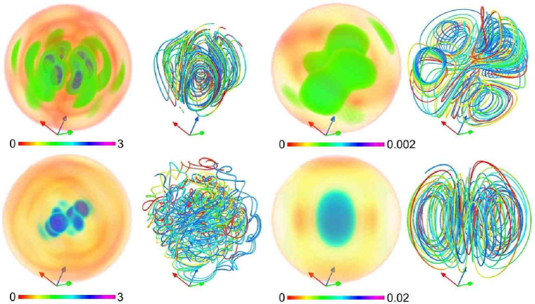
Figure 7: Above: kinetic energy density and velocity field lines in run II, at $t=1.5$ (left) and at $t=15$ (right). Below: magnetic energy density and magnetic field lines in the same run, at $t=1.5$ (left) and at $t=15$ (right). For convenience, intensity and field lines are always shown in pairs, with intensity on the left and field lines on the right.

Based on the definition of the energy spectrum, we can also introduce an energy-containing lengthscale as

$$\ell=\frac{R\,\min\{|\lambda|\}}{E}\int{E(|\lambda|)|\lambda|^{-1}\,{\textrm{d}}|\lambda|},$$ (26)

and a Taylor lengthscale

$$\lambda_{T}=R\,\min\{|\lambda|\}\left[E\bigg{/}\int{E(|\lambda|)|\lambda|^{2}\,{\textrm{d}}|\lambda|}\right]^{1/2},$$ (27)

where $E$ is the energy, and $E(|\lambda|)$ is the energy spectrum as a function of $|\lambda|$ (the sums are represented symbolically as integrals). Using the kinetic and magnetic energies, these characteristic lengths can be computed for the velocity and magnetic fields. In both runs, at $t=0$ $\ell\approx\lambda_{T}\approx 0.33$ for both fields. As the system evolves these quantities grow monotonically, but while at $t=20$ for the velocity field $\ell\approx 0.5$, for the magnetic field $\ell\approx 1$. As a criterion to decide if the simulations were well resolved in spectral space, the scales where the kinetic and magnetic enstrophy spectrum peaked were observed as a function of time, and it was asked that their corresponding wavenumbers $|\lambda|$ were smaller than $\max\{|\lambda|\}$ at all times.

Figure 6 shows the amplitude of the individual modes $\xi^{B}$ in run II at $t=10$ as a function of $q$ and $l$ (all values of $m$ for each value of $l$ are summed). Most of the magnetic energy is concentrated in the shell with $l=1$, and the modes with $q=\pm 1$ in this shell have the largest amplitude. Note the imbalance between the mode with $q=1$ and $q=-1$, indicating some helicity is present in the magnetic field.

The dominance of a helical large scale magnetic field at late times can also be identified in an inspection of the fields in configuration space. Figure 7 shows field intensity and field lines for the velocity and magnetic field at $t=1.5$ (left) and $t=15$ (right) in run II. While at early times both fields show small scale features, at late times the velocity field looks reminiscent of a quadrupole and the magnetic field looks like a dipole oriented roughly in the $z$ direction. However, the magnetic field at $t=15$ is helical and the magnetic field lines are not purely poloidal. There is a small toroidal component to the magnetic field, and the magnetic field lines proceed slowly in the $\phi$-direction in a helical fashion.

In Fig. 7 and in the following visualizations the labels are as follows. The $x$, $y$, and $z$ directions are indicated by the arrows (in the online version, these are respectively red, green, and blue). The color and opacity are proportional to the field intensity, colorbars are given as a reference. Field lines are computed taking a snapshot of the field at a fixed instant in time, and integrating a trajectory from twenty random points in the surroundings of the center of the sphere. The field is not evolved in time as the lines are integrated. To indicate the direction of the fields, in the online version the lines change color according to the distance integrated from the initial point; from red to yellow, and finally blue.

V DYNAMO EFFECT

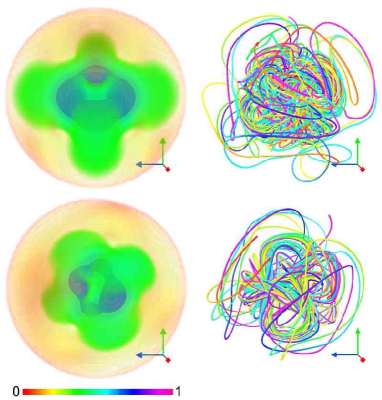
Figure 8: Intensity of the forcing function ${\bf f}$ used in the dynamo simulations (left), and associated field lines (right). Above: function used in run III. Below: function used in runs IV and V.

Figure 9: Kinetic (dashed line) and magnetic energy (solid line) as a function of time in run III.

Figure 10: Trace of the magnetic dipole orientation on the unit sphere (above) and magnitude of the dipole moment as a function of time (below) in run III.

In an MHD dynamo, an initially small “seed” magnetic field is amplified and sustained against Ohmic dissipation solely by the motions of a conducting fluid. Magnetic fields observed in planets and stars are believed to be the result of a dynamo process. The mechanical mechanisms proposed vary widely, including thermal convection, Ekman pumping due to rotation, precession, irregularities on the inner surface of the planetary mantles, and so on. In this Section, we study three simple examples of forced dynamo action in the sphere with relatively simple realizations of the forcing function ${\bf f}$ of Eq. (5). Figure 8 shows visualizations of the two expressions used for ${\bf f}$. The geometry of the forcing function is not intended to mimic any particular process in the planetary or stellar dynamos, but is rather inspired in a common practice in dynamo simulations with periodic boundary conditions: a few spectral modes are forced in the mechanical energy, and for Reynolds numbers large enough generic properties of the simulations are studied.

In all cases to be described here, a purely hydrodynamic (${\bf B}=0$) computation was carried out first until a steady state (laminar or turbulent) was reached for the velocity field. The amplitude of ${\bf f}$ was chosen to have rms velocity of order one in the steady state. Then a random magnetic field with energy $E_{M}\sim 10^{-6}$ was loaded into the modes with $|q|=l=4$. The simulations were then continued in order to observe the amplification and subsequent development of the magnetic field.

Three dynamo simulations were done in which the Reynolds numbers and the number of modes excited were progressively increased. In the first case, the system reaches a steady state with a stable dipole moment which varies little in time. In the second case, the dipole moment forms, then spontaneously changes direction. In the third, the Reynolds number is high enough that the velocity field might be called turbulent, and many modes are excited; for this case, the dipole moment changes erratically in time.

A resolution of $\max\{|q|\}=\max\{l\}=9$ was used in all the runs. The same criteria as in the previous section was used to decide if a simulation was well resolved. For the last run, a simulation with higher resolution was also carried out to see if the results would be modified by the change in resolution.

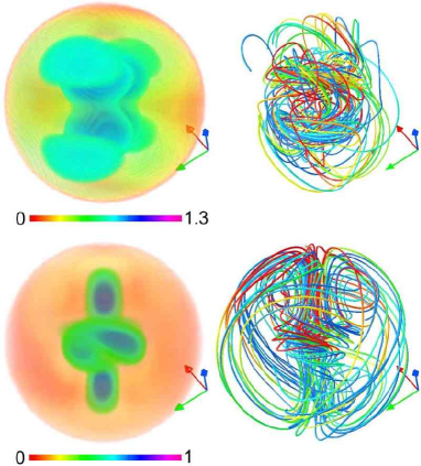
Figure 11: Above: kinetic energy density and velocity field lines in run III, at $t=915$. Below: magnetic energy density and magnetic field at the same time. The same conventions than in Fig. 7 are used.

V.1 Laminar runs

In this section we present results from two runs with $\nu=\eta=3\times 10^{-3}$. In run III, the external forcing ${\bf f}$ in Eq. (5) is given by the coefficient

$$\xi^{f}_{2,2,1}=f_{0}(1+i),$$ (28)

with $f_{0}=1.4$, which corresponds to one C-K mode and as a result injects maximum kinetic helicity in the system. In run IV, the external forcing is

$$\xi^{f}_{2,2,0}=5\xi^{f}_{-2,2,0}=f_{0},$$ (29)

$$\xi^{f}_{2,2,m}=5\xi^{f}_{-2,2,m}=f_{0}(1+i),$$ (30)

where $m$ runs from 1 to 2 and negative values of $m$ are again given by $\xi_{q,l,-m}=(-1)^{m}\xi^{*}_{qlm}$. The amplitude of the forcing is $f_{0}=0.9$. This forcing injects non-maximal kinetic helicity (plus, of course, kinetic energy) into the system. Figure 8 shows visualizations of the two forcing functions in configuration space. In both cases the forcing is stronger in the center of the sphere, and a modulation due to $m=2$ modes in the forcing can be easily identified. The phase and amplitude of the external force ${\bf f}$ were kept constant during the entire simulations.

Figure 9 shows the time history of the magnetic and kinetic energy in run III. The Reynolds numbers based on the length $R=1$ and the rms velocity are $R_{V}=R_{M}\approx 290$, and the energy containing scale of the flow is $\ell\approx 0.5$. Before the magnetic field is introduced, only the forced mode is excited.

After the magnetic seed is introduced, the magnetic energy is amplified exponentially in a kinematic regime. Then the magnetic field saturates around $t\approx 150$ and the Lorentz force quenches the velocity field. In the final steady state, more mechanical modes besides the forced mode are excited. This is the result of an instability of the flow, triggered by the Lorentz force as the magnetic field grows exponentially.

Figure 10 shows the trace of the orientation of the dipole moment in the surface of the unit sphere, and the magnitude of the dipole moment as a function of time for run III. The dipole moment grows during the kinematic regime, but its orientation changes erratically in time. At $t\approx 200$ $|\mbox{\boldmath$\mu$}|$ reaches its maximum amplitude and converges slowly to a steady state. Also it direction changes slowly, and after $t\approx 400$ almost no change is observed. At late times the dipole shows no inclination toward further systematic dynamical development.

Figure 12: Kinetic (dashed line) and magnetic energy (solid line) as a function of time in run IV.

Figure 13: Trace of the magnetic dipole orientation on the unit sphere (above) and magnitude of the dipole moment as a function of time (below) in run IV.

A visualization of the velocity and magnetic fields in configuration space in the steady state of run III is shown in Fig. 11. The kinetic energy is concentrated in two counter-rotating regions, located in the center of each hemisphere. Note the $m=2$ modulation in the forcing is still visible in the kinetic energy density. The velocity field in these regions is mostly toroidal, as indicated by the velocity field lines. The magnetic energy is larger in the center of the sphere, and along the axis defined by the two counter-rotating eddies. In the interior, but away from the axis, magnetic field lines are mostly toroidal, as the result of the stretching by the two counter-rotating eddies. Along the axis and close to the boundaries, the flow is mostly poloidal.

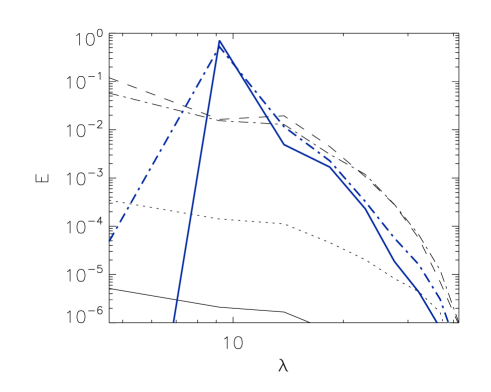
Figure 14: Kinetic energy spectrum at $t=52$ [thick (blue) solid line] and at $t=500$ [thick (blue) dash-dotted line] in run IV; the thin lines correspond to the magnetic energy spectrum at $t=52$ (solid), $t=82$ (dotted), $t=250$ (dashed), and $t=500$ (dash-dotted).

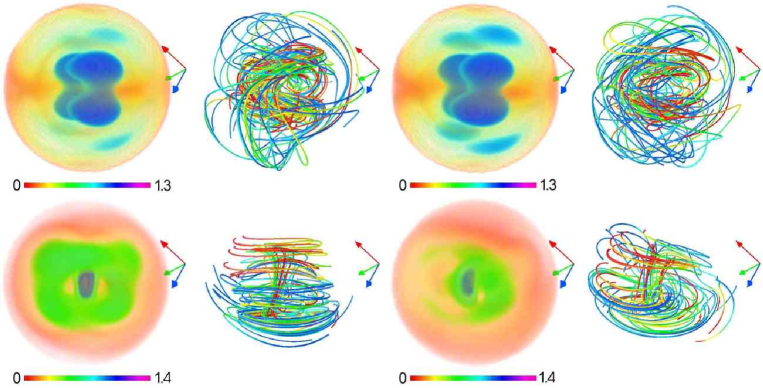
Figure 15: Above: kinetic energy density and velocity field lines in run IV, at $t=315$ (left) and at $t=1065$ (right). Below: magnetic energy density and magnetic field lines in the same run, at $t=315$ (left) and at $t=1065$ (right). The same conventions than in Fig. 7 are used.

The time history of the kinetic and magnetic energy in run IV is shown in Fig. 12. The Reynolds numbers for this run (based on the length $R=1$) are $R_{V}=R_{M}\approx 280$, and the energy containing scale of the flow is $\ell\approx 0.48$. Although the kinematic viscosity and magnetic diffusivity are the same as in run III, the external forcing injects energy in a larger number of modes and even before the magnetic field is introduced non-forced modes have some mechanical energy. After the magnetic seed is introduced, the magnetic energy grows exponentially until at $t\approx 150$ saturates. The system seems to reach a steady state but suddenly at $t\approx 500$ the magnetic energy decreases by a factor of $\approx 1.8$, the kinetic energy increases by $\approx 1.1$, and the system reaches a second steady state.

Figure 16: Kinetic (dashed line) and magnetic energy (solid line) as a function of time in run V.

Figure 17: Time evolution of the three components of the dipole moment in run V. Labels are as in Fig. 10.

The abrupt change in the kinetic and magnetic energy in run IV at $t\approx 500$ is associated with a reorientation of the magnetic dipole moment. Figure 13 shows the time evolution of the direction and amplitude of $\mu$. As in run III, in the kinematic stage the dipole moment grows rapidly and its direction fluctuates erratically, until reaching a first quasi-steady state at $t\approx 200$. The dipole moment then stays approximately constant until at $t\approx 400$ the magnetic field evolves rapidly, and the dipole moment changes direction to a second attractor (reached at $t\approx 600$). The angle the dipole flips by is close to $\pi/2$. After $t\approx 600$ only a slow change in $\mu$ is observed. The amplitude of the dipole moment also changes rapidly as the dipole shifts at $t\approx 400$; while at $t\approx 300$ $|\mbox{\boldmath$\mu$}|\approx 0.36$, at $t\approx 1000$ $|\mbox{\boldmath$\mu$}|\approx 0.54$.

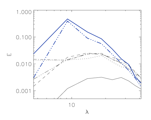
Figure 18: Kinetic energy spectrum at $t=75$ [thick (blue) solid line] and at $t=600$ [thick (blue) dash-triple dotted line] in run V; the thin lines correspond to the magnetic energy spectrum at $t=75$ (solid), $t=168$ (dotted), $t=240$ (dashed), $t=544$ (dash-dotted), and $t=500$ (dash-triple dotted).

Figure 14 shows the kinetic and magnetic energy spectra in run IV at different times. The kinetic energy spectrum peaks at $|\lambda|\approx 9$, corresponding to the forced modes with $q=2$ and $l=2$. The energy in the remaining modes is at least two orders of magnitude smaller than in the forced modes. At late times, some kinetic energy is excited in the largest available scale, as well as a small angular momentum ($|{\bf L}|^{2}/E_{V}\approx 1.5\times 10^{-4}$ after $t\approx 600$). The angle between the dipole moment and this small angular momentum remains constant after $t=100$ and is $\pi/2$. Visualizations of the velocity and magnetic fields in configuration space are shown in Fig. 15. The geometry of the velocity field is more complex than in run III, although the $m=2$ modulation in the kinetic energy can still be recognized. Note at $t=315$ the magnetic field lines are mostly poloidal in the center of the sphere, and toroidal close to the boundary. The change in the orientation of $\mu$ at $t\approx 400$ takes place without a strong change in the velocity field, and a relatively small change in the magnetic field configuration.

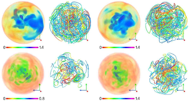
Figure 19: Above: kinetic energy density and velocity field lines in run V, at $t=75$ (left) and at $t=1035$ (right). Below: magnetic energy density and magnetic field lines in the same run, at $t=75$ (left) and at $t=1035$ (right). We were unable to find an ordered pattern in either field.

V.2 A rapidly-varying dipole

For run V, the external forcing f is given by Eqs. (29) and (30), but the kinematic viscosity and magnetic diffusivity are dropped to $\nu=\eta=3\times 10^{-4}$. The resulting kinetic and magnetic Reynolds numbers based on the length $R=1$ are $R_{V}=R_{M}\approx 2300$, and the energy-containing and Taylor scales are respectively $\ell\approx 0.4$ and $\lambda_{T}=0.35$.

The evolution of the kinetic and magnetic energy in run V is shown in Fig. 16. Again, after an initial kinematic regime where the magnetic energy is amplified exponentially, the system reaches a statistical steady state. Note that in this simulation both the kinetic and magnetic energy fluctuate strongly with time, indicating the nonlinear coupling between modes is stronger than in runs III and IV, as a result of the higher Reynolds numbers.

Figure 17 shows the trace of the dipole moment in the surface of the unit sphere, and its intensity as a function of time, in run V. The direction of $\mu$ appear to fluctuate randomly, changing hemisphere with a characteristic time of the order of 100 eddy turnover times. In the meantime, the whole surface of the unit sphere seems to be explored by the fluctuations in $\mu$. The angular momentum is small and fluctuates around $|{\bf L}|^{2}/E_{V}\approx 5\times 10^{-3}$. However, unlike in Run III, in this simulation the angle between the dipole moment and the angular momentum is not even approximately constant and fluctuates seemingly randomly between $0$ and $\pi$. The question of under what circumstance the dipole favors one or another alignment appears to be quite unsettled, and deserves further study in higher-resolution simulations with larger angular momentum and rotation.

The kinetic and magnetic energy spectra in run V at several times are shown in Fig. 18. More modes are excited in the velocity field, in accordance with the strong fluctuations in time observed in the kinetic energy. While in runs III and IV the magnetic energy spectrum peaks at large scales even during the kinematic regime, in run V at early times the magnetic energy peaks at scales smaller than the forcing scale. Also, after the nonlinear saturation of the dynamo, a fluctuation in the amplitude of the large scale magnetic field is observed. The minima are correlated with times of minima of $\mu^{2}$, when the three components of the dipole moment fluctuate around zero. Most of the activity in this run is in small scales and fluctuations in the flow are larger than in runs III and IV. Even at late times when a large scale magnetic field has developed, intermediate scales give a large contribution to the magnetic energy. This also explains the strong fluctuations observed in the dipole moment. Since $\mu$ is proportional to the current density, the small scales give a large contribution to the dipole moment.

Figure 19 shows the magnetic and velocity field in real space at two different times in run V. The fields have more small scale structure than in run IV. Any trace of the $m=2$ modulation of the forcing has been completely lost. Also, in the kinematic regime (see e.g. the magnetic field at $t=75$) the magnetic energy is mostly in the small scales, as also indicated by the magnetic energy spectrum.

VI DISCUSSION

We have introduced some computational machinery that is intended for a quantitative discussion of nonlinear and incompressible magnetohydrodynamics inside a sphere for a wide range of initial conditions and varieties of mechanical forcing. It is concerned essentially with the analytical and computational aspects of dynamo action in this geometry in a somewhat abstract setting, and is not the same as periodic dynamo computations with rectangular symmetry, or with planetary-dynamo or solar-dynamo computations whose central focus is reproduction of observations of magnetic behavior of a real system. There are other features yet to be included and it is our intent to introduce them one at a time: rigid rotation and Ekman pumping, an insulating but non-conducting boundary to permit the magnetic field’s penetration into the surrounding vacuum region, and different forms of mechanical excitations.

The operation of the wholly spectral code, which has had a precedent in axially periodic circular-cylinder geometry has been illustrated by a few simple examples, not in any sense a comprehensive study. First, decaying turbulence has been studied involving the relaxation of helical initial conditions to a magnetically dominated state whose spectrum is dominated by the longest allowed spatial scales and whose kinetic energy is essentially gone. Also, dynamo computations have been done for three successively higher sets of Reynolds numbers, revealing a different magnetic behavior in each case. In the first case, a magnetic dipole formed in what was essentially a laminar velocity field and appears willing to persist for as long as the code is run. In the second case, another dipole formed, but after the passage of a few hundred large-scale eddy-turnover times, it changed its magnitude to a somewhat larger value, and flipped its orientation, for reasons we do not know but that are worth exploring. These fluctuations have required neither a preferred direction enforced by rigid rotation nor thermally convective rolls. Finally, in the third case, the velocity field had Reynolds numbers (based on the radius of the sphere) of about $2300$ and could be said to be turbulent. In this turbulent case, there was a dipole moment, but it exhibited no systematic or regular behavior as far as we could tell, and changed its orientation from one hemisphere to the other every $100$ or so eddy turnover times, exploring in the meantime all possible orientations. It did appear to be a resolved computation, despite the turbulence, and we believe represents a bona fide solution of the MHD equations. All these runs, it should be stressed, were carried out with a magnetic Prandtl number of unity, and may well change for values far from that. One outcome to be noted is that neither turbulence nor rotation have been a necessary ingredient for the development and maintenance of a magnetic dipole, but the presence of mechanically helicity has helped a lot. Spontaneous changes in magnetic dipole orientation have been easy to observe, both in laminar and turbulent cases.

We should also stress that the code as presently constituted is limited to a relatively small number of degrees of freedom, far fewer than well-resolved high Reynolds number mechanical turbulence would demand. It will also be attempted to design wall-friction terms to permit a more efficient exchange of angular momentum from the fluid to the wall Shan94 , once rigid rotation is introduced. Also rigid rotation and different boundary conditions for the magnetic fields can be implemented. Given the properties and limitations of the method described (purely spectral, non-dispersive, and conservative), we believe this method can be used as a testbed to explore the effect of different physical effects, boundary conditions, subgrid models (several models, such as the Lagrangian averaged model Holm02a ; Holm02b ; Mininni05d are easier to implement in spectral space), etc., before trying these ideas in more complex and realistic codes to reach high Reynolds numbers.

- (1) H. K. Moffatt, Magnetic field generation in electrically conducting fluids. Cambridge, Cambridge Univ. Press (1978).
- (2) G. A. Glatzmaier and P. H. Roberts, “A three-dimensional self-consistent computer simulation of a geomagnetic field reversal,” Nature 377, 203–209 (1995).
- (3) M. Dikpati and P. Charbonneau, “A babcock-leighton flux transport dynamo with solar-like differential rotation,” Astrophys. J. 518, 508–520 (1999).
- (4) M. Kono and P. H. Roberts, “Recent geodynamo simulations and observations of the geomagnetic field,” Rev. Geophys. 40, 1–53 (2002).
- (5) D. Nandy and A. R. Choudhuri, “Explaining the latitudinal distribution of sunspots with deep meridional flow,” Science 296, 1671–1673 (2002).
- (6) P. D. Mininni and D. O. Gómez, “A new technique for comparing solar dynamo models and observations,” Astron. Astrophys. 426, 1065–1073 (2004).
- (7) A. Gailitis, O. Lielausis, E. Platacis, S. Dement’ev, A. Cifersons, G. Gerbeth, T. Gundrum, F. Stefani, M. Christen, and G. Will, “Magnetic field saturation in the riga dynamo experiment,” Phys. Rev. Lett. 86, 003024 (2001).
- (8) R. Steiglitz and U. Müller, “Experimental demonstration of a homogeneous two-scale dynamo,” Phys. Fluids 13, 561–564 (2001).
- (9) K. Noguchi, V. I. Pariev, S. A. Colgate, H. F. Beckley, and J. Nordhaus, “Magnetorotational instability in liquid metal couette flow,” Astrophys. J. 575, 1151–1162 (2002).
- (10) F. Pétrélis, M. Bourgoin, L. Marié, J. Burguete, A. Chiffaudel, F. Daviaud, S. Fauve, P. Odier, and J.-F. Pinton, “Nonlinear magnetic induction by helical motion in a liquid sodium turbulent flow,” Phys. Rev. Lett. 90, 174501 (2003).
- (11) D. R. Sisan, W. L. Shew, and D. P. Lathrop, “Lorentz force effects in magneto-turbulence,” Phys. Earth Plan. Int. 135, 137–159 (2003).
- (12) E. J. Spence, M. D. Nornberg, C. M. Jacobson, R. D. Kendrick, and C. B. Forest, “Observation of a turbulence-induced large scale magnetic field,” Phys. Rev. Lett. 96, 055002 (2006).
- (13) P. H. Roberts and G. A. Glatzmaier, “The geodynamo, past, present and future,” Geophys. Astrophys. Fluid Dyn. 94, 47–84 (2001).
- (14) A. Brandenburg and K. Subramanian, “Astrophysical magnetic fields and nonlinear dynamo theory,” Phys. Rep. 417, 1–209 (2005).
- (15) Y. Ponty, P. D. Mininni, D. C. Montgomery, J.-F. Pinton, H. Politano, and A. Pouquet, “Numerical study of dynamo action at low magnetic prandtl numbers,” Phys. Rev. Lett. 94, 164502 (2005).
- (16) P. D. Mininni, Y. Ponty, D. C. Montgomery, J.-F.Pinton, H. Politano, and A. Pouquet, “Dynamo regimes with a nonhelical forcing,” Astrophys. J. 626, 853–863 (2005).
- (17) P. D. Mininni and D. C. Montgomery, “Low magnetic prandtl number dynamos with helical forcing,” Phys. Rev. E 72, 056320 (2005).
- (18) A. Alexakis, P. D. Mininni, and A. Pouquet, “Shell-to-shell energy transfer in magnetohydrodynamics. i. steady state turbulence,” Phys. Rev. E 72, 046301 (2005).
- (19) P. D. Mininni, A. Alexakis, and A. Pouquet, “Shell-to-shell energy transfer in magnetohydrodynamics. ii. kinematic dynamo,” Phys. Rev. E 72, 046302 (2005).
- (20) S. Chandrasekhar and P. C. Kendall, “On force-free magnetic fields,” Astrophys. J. 126, 457–460 (1957).
- (21) L. Turner, “Statistical mechanics of a bounded, ideal magnetofluid,” Ann. Phys. (NY) 149, 58–161 (1983).
- (22) Z. Yoshida, “Discrete eigenstates of plasmas described by the chandrasekhar-kendall functions,” Prog. Theor. Phys. 86, 45–55 (1991).
- (23) Z. Yoshida, “Eigenfunction expansions associated with the curl derivatives in cylindrical geometries: Completeness of chandrasekhar-kendall,” J. Math. Phys. 33, 1252–1256 (1992).
- (24) J. Cantarella, D. DeTurck, H. Gluck, and M. Teytel, “The spectrum of the curl operator on spherically symmetric domains,” Phys. Plasmas 7, 2766–2775 (2000).
- (25) C. Mueller, Foundations of the mathematical theory of electromagnetic waves. New York, Springer Verlag (1969).
- (26) D. C. Montgomery, L. Turner, and G. Vahala, “Three-dimensional magnetohydrodynamic turbulence in cylindrical geometry,” Phys. Fluids 21, 757–764 (1978).
- (27) X. W. Shan, D. Montgomery, and H. D. Chen, “Nonlinear magnetohydrodynamics by galerkin-method computation,” Phys. Rev. A 44, 6800–6818 (1991).
- (28) X. W. Shan and D. Montgomery, “On the role of the hartmann number in magnetohydrodynamic activity,” Plasma Phys. Cont. Fus. 35, 619–631 (1993).
- (29) X. W. Shan and D. Montgomery, “Global searches of hartmann-number-dependent stability boundaries,” Plasma Phys. Cont. Fus. 35, 1019–1032 (1993).
- (30) X. W. Shan and D. Montgomery, “Magnetohydrodynamic stabilization through rotation,” Phys. Rev. Lett. 73, 1624–1627 (1994).
- (31) S. J. Li and D. Montgomery, “Decaying two-dimensional turbulence with rigid walls,” Phys. Lett. A 218, 281–291 (1996).
- (32) S. J. Li, D. Montgomery, and W. B. Jones, “Two-dimensional turbulence with rigid circular walls,” Theor. Comp. Fluid Dyn. 9, 167–181 (1997).
- (33) B. T. Kress and D. C. Montgomery, “Pressure determinations for incompressible fluids and magnetofluids,” J. Plasma Phys. 64, 371–377 (2000).
- (34) G. Gallavotti, Foundations of fluid dynamics. Berlin, Springer Verlag (2002), pp. 83–87 ff.
- (35) J. Clyne and M. Rast, “A prototype discovery environment for analyzing and visualizing terascale turbulent fluid flow simulations,” in Visualization and data analysis 2005 (R. F. Erbacher, J. C. Roberts, M. T. Grohn, and K. Borner, eds.), pp. 284–294, SPIE, Bellingham, Wash. (2005).
- (36) D. J. Ivers and C. G. Phillips, “A vector spherical harmonic spectral code for linearised magnetohydrodynamics,” ANZIAM J. 44, C423–C442 (2003).
- (37) W. H. Press, B. P. Flannery, S. A. Teukolsky, and W. T. Vetterling, Numerical Recipes in FORTRAN 77. Cambridge, Cambridge Univ. Press (1992).
- (38) C. Canuto, Y. Hussaini, A. Quarteroni, and T. Zang, Spectral methods in fluid dynamics. New York, Springer Verlag (1988).
- (39) W. H. Matthaeus and D. Montgomery, “Selective decay hypothesis at high mechanical and magnetic reynolds numbers,” Ann. N. Y. Acad. Sci. 357, 203 (1980).
- (40) A. C. Ting, W. H. Matthaeus, and D. Montgomery, “Turbulent relaxation processes in magnetohydrodynamics,” Phys. Fluids 29, 3261–3274 (1986).
- (41) R. Kinney, J. C. McWilliams, and T. Tajima, “Coherent structures and turbulent cascades in two-dimensional incompressible magnetohydrodynamic turbulence,” Phys. Plasmas 2, 3623–3639 (1995).
- (42) P. D. Mininni, D. C. Montgomery, and A. Pouquet, “Numerical solutions of the three-dimensional magnetohydrodynamic model,” Phys. Rev. E 71, 046304 (2005).
- (43) D. D. Holm, “Averaged lagrangians and the mean effects of fluctuations in ideal fluid dynamics,” Physica D 170, 253–286 (2002).
- (44) D. D. Holm, “Lagrangian averages, averaged lagrangians, and the mean effects of fluctuations in fluid dynamics,” Chaos 12, 518–530 (2002).