Controlling chaos in spatially extended beam-plasma system by the continuous delayed feedback

Abstract

In present paper we discuss the control of complex spatio-temporal dynamics in a spatially extended non-linear system (fluid model of Pierce diode) based on the concepts of controlling chaos in the systems with few degrees of freedom. A presented method is connected with stabilization of unstable homogeneous equilibrium state and the unstable spatio-temporal periodical states analogous to unstable periodic orbits of chaotic dynamics of the systems with few degrees of freedom. We show that this method is effective and allows to achieve desired regular dynamics chosen from a number of possible in the considered system.

The problem of controlling dynamics of non-linear dynamical systems by stabilization of existing unstable periodical orbits divides into two tasks. The first of them is picking out and analysing the periodical states. For this purpose the algorithm of Lathrop and Kostelich and algorithm of Schmelcher and Diakonos (SD–method) are often used. The second task is stabilization of unstable orbit. In distributed systems the role of unstable orbits is performed by spatio-temporal periodical states. In our work we propose methods of picking out unstable periodical spatio-temporal states with the help of modified Kostelich and SD–methods for distributed beam-plasma systems. Stabilization is realized with the help of continuous delayed feedback, by the method based on Pyragas works. The most attractive feature of the proposed method is that the continuous control signal is given to one of the boundaries of the system what makes this method convenient to use in practice, for example, for microwave beam-plasma systems.

Introduction

Practical use of unstable periodic orbits of chaotic attractor for chaos controlling has been discussed in a number of papers since the the work of E. Ott, C. Grebogy, J. Yorke E. Ott, C. Grebogi, J.A. Yorke (1990) has been published. In the works S. Boccaletti, C. Grebogi, Y.-C. Lai, H. Mancini, D. Maza (2000); C. Grebogi, E. Ott, J.A. Yorke (1988); D.P. Lathrop, E.J. Kostelich (1989); P. Schmelcher, F.K. Diakonos (1997); M. Dhamala, Y.-Ch. Lai (1999); T.L. Carroll (1999); J.A.C. Gallas (2001); D. Pingel, P. Schmelcher, F.K. Diakonos (2001) it has been shown that unstable orbits of chaotic attractor of a dynamical system with few degrees of freedom can be used to control complex behaviour of the system, and the stabilization of the unstable periodic orbit needs small perturbation of the system dynamics. The work E. Ott, C. Grebogi, J.A. Yorke (1990) offers an algorithm of chaos control, defining the change of the system parameter in the dependence of the distance between the current state of the system and the wanted orbit. The value and sign of the parameter change can be discussed as the signal of some feedback. This method can also be applied to flow systems.

As it has been shown in a number of works W.L. Ditto, S.N. Rauseo, M.L. Spano (1990); E.R. Hunt (1991); S. Bielawski, D. Derozier, P. Glorieux (1993); T. Shinbrot, E. Ott, C. Grebogi, J.A. Yorke (1993) the OGY algorithm is insensitive to noise and inexact knowledge of the system state and it can be applied to the systems with finite, but large degrees of freedom M. Ding, W. Yang, V. In, W.L. Ditto (1996).

But it seems rather hard to apply the OGY algorithm to control the dynamics of different distributed chaotic systems, including one we are discussing in this work, because it demands the explicit knowledge of system state and the quick change of control parameter along the whole system space. It is nearly impossible to realize in real microwave beam-plasma systems working in the frequency rang $0.1\div 100$ GHz.

For such systems it seems more prospective to use the method of stabilization of the unstable periodic states suggested by K. Pyragas K. Pyragas (1992). In this work the continuous Y.H. Chen, M.Y. Chou (1994), and not discrete quickly changing feedback is used, what makes this algorithm appropriate for the distributed microwave systems. In the Pyragas scheme the system is synchronized with its own state taken one orbit period earlier, by continuous change of control parameter $\varepsilon(t)=\gamma({\xi(t)-\xi(t-T)})$, where $\xi(t)$ is the analyzed variable, $\gamma$ is the feedback coefficient and $T$ is the orbit period. When the stabilization of the unstable orbit takes place, the feedback signal has the order of the noise level. It is important that all the information demanded for stabilization, except for $T$ and $\gamma$, is contained in the time series of the system dynamics $\xi(t)$, i.e. is defined automatically in real time. Applications of such controlling scheme were theoretically and practically investigated in different systems and models S. Boccaletti, C. Grebogi, Y.-C. Lai, H. Mancini, D. Maza (2000); Y.H. Chen, M.Y. Chou (1994); D.J. Gauthier, D.W. Sukow, H.M. Concannon, J.E.S. Socolar (1994); Franz-Josef Elmer (1998); Y.C. Kouomou, P. Woafo (2002) including laser physics R. Roy, T.W. Murphy, T.D. Maier, Z. Gills, E.R. Hunt (1992); R. Meucci, W. Gadomski, M. Ciofini, F.T. Arecchi (1994); R. Meucci, M. Ciofini, R. Abbate (1996), models of geophysical processes E. Tziperman, H. Scher, S.E. Zebiak, M.A. Cane (1997) and the processes of “reaction–diffusion” G. Franceschini, S. Bose, E. Schöll (1999).

We must mark especially that this scheme with continuous feedback has been used for controlling spatio-temporal chaos in distributed systems (see for example works G. Franceschini, S. Bose, E. Schöll (1999); W. Lu, D. Yu, R.G. Harrison (1996); R. Martin, A.J. Scroggie, G.-L. Oppo, W.J. Firth (1996) devoted to stabilization of two-dimensional structures in the $2D$ distributed chaotic system, described by partial derivative equations; works H. Gang, QuZhilin, (1994); R.O. Grigoriev, M.C. Cross, H.G. Schuster (1997); P. Parmananda, M. Hildebrand, M. Eiswirth (1997), in which chaos control in the lattices of coupled maps has been considered; the works analyzing such sample equations as the complex Ginzburg-Landau equation in non-linear dynamics R. Montagne, P. Colet (1997); S. Boccaletti, J. Bragard, F.T. Arecchi (1999) or the Swift-Hohenberg equation of laser physics M.E. Bleich, D. Hochheiser, J.V. Moloney, J.E.S. Socolar (1997); D. Hochheiser, J.V. Moloney, J. Lega (1997)). Among such investigations we must mark works S. Boccaletti, J. Bragard, F.T. Arecchi (1999); G. Franceschini, S. Bose, E. Schöll (1999) especially. Thus, in the work of Boccaletti S. Boccaletti, J. Bragard, F.T. Arecchi (1999) the problem of chaos control in the Ginzburg-Landau model with the use of a large (but finite) number of small local perturbations has been investigated. This method allows to stabilize the unstable structures of chaotic spatio-temporal dynamics and to synchronize two chaotic states. Franceschini and the others in work G. Franceschini, S. Bose, E. Schöll (1999) studied the problem of controlling chaotic generation of impulses in the model of uniformly coupled “reaction–diffusion” systems used for describing the processes of charge transfer in bistable semiconductor. The controlling feedback signal in mathematical model offered in work G. Franceschini, S. Bose, E. Schöll (1999) is supposed to be spatially homogeneous, i.e. the perturbation carried into every point of the system space is the same.

Some works describing chaos control in microwave beam–plasma systems must also be mentioned. The stabilization of unstable periodic orbits in a fluid model of Pierce diode with the help of the OGY algorithm has been discussed in work N. Krahnstover et al (1998). Work H. Friedel, R. Grauer, H.K. Spatschek (1998) discusses the problem of suppression of the regime of the virtual cathode in Pierce diode J. Pierce (1944); H. Matsumoto, H. Yokoyama, D. Summers (1996) with the help of delayed feedback using a numerical method of large particles. In our work A.E. Hramov, I.S. Rempen (2004) the influence of the external feedback on the chaotic oscillations in Pierce diode has been examined.

It is important to note, that in the majority of works devoted to chaos control in the distributed systems, the controlling feedback signal effects at every point of the system space. Such distributed spatio-temporal control can be used, for example, in optical systems A.V. Mamaev, M. Saffman (1998); L. Pastur, L. Gostiaux, U. Bortolozzo, S. Boccaletti, P.L. Ramazza (2004); F. T. Arecchi, S. Boccaletti, P. L. Ramazza, and S. Residori (2004). But application of such methods to beam-plasma systems causes several difficulties. In the present work we propose a method of chaos control based on the continuous feedback scheme, where the feedback signal is given to one of the boundaries of the distributed system. As a sample this method is applied to widely known simple distributed beam-plasma system (fluid model of Pierce diode)

As it has already been mentioned above, the knowledge of the positions of the unstable orbits in the phase space and their periods is quite important for controlling chaos in the discrete and flow systems with a small number of degrees of freedom. We can say that in distributed systems the unstable periodic spatio-temporal states play the roles of unstable orbits. Therefore, for the efficient chaos controlling we need to find such unstable periodic states. Accordingly, we propose a simple method of detecting of unstable periodic spatio-temporal states and their further stabilization.

The structure of the paper is following: In Section I the fluid model of Pierce diode is discussed. In Section II stabilization of the unstable homogeneous equilibrium state is described. In Section III the spatio-temporal data series of electron beam dynamics are analyzed and the unstable periodic spatio–temporal states of the chaotic dynamics are carried out. And, in Section IV we discuss the stabilization of the unstable periodic spatio-temporal states (unstable states) derived in Section III, with the help of feedback of different type. In conclusion we summarize the main results discussed in our paper.

I General formalism

Pierce diode J. Pierce (1944); H. Matsumoto, H. Yokoyama, D. Summers (1996) is one of the simplest beam-plasma systems demonstrating complex chaotic dynamics B.B. Godfrey (1987); S. Kuhn, A. Ender (1990); P.A. Lindsay, X. Chen, M. Xu (1995); H. Matsumoto, H. Yokoyama, D. Summers (1996); A.E. Hramov, I.S. Rempen (2004). It consists of two plane parallel infinite grids pierced by the monoenergetic (at the entrance) electron beam (see Fig. 1). The grids are grounded and the distance between them is $L$. The entrance space charge density $\rho_{0}$ and velocity $v_{0}$ are maintained constant. The space between the grids is evenly filled by the neutralizing ions with density $|\rho_{i}/\rho_{0}|=1$. The dynamics of this system is defined by the only parameter, the so-called Pierce parameter

$$\alpha={\omega_{p}L}/{v_{0}},$$ (1)

where $\omega_{p}$ is the plasma frequency of the electron beam. With $\alpha>\pi$ in the system, the so-called Pierce instability J. Pierce (1944); H. Matsumoto, H. Yokoyama, D. Summers (1996) develops, which leads to the appearance of the virtual cathode. At the same time, with $\alpha\sim 3\pi$, the instability is limited by non-linearity and the regime of complete passing of the electron beam through the diode space can be observed. In this case the system can be described by the fluid equations:

$$\frac{\partial v}{\partial t}+v\frac{\partial v}{\partial x}=\frac{\partial\varphi}{\partial x},$$ (2)

$$\frac{\partial\rho}{\partial t}+v\frac{\partial\rho}{\partial x}+\rho\frac{\partial v}{\partial x}=0,$$ (3)

$$\frac{\partial^{2}\varphi}{\partial x^{2}}=\alpha^{2}(\rho-1),$$ (4)

with the boundary conditions:

$$v(0,t)=1,\quad\rho(0,t)=1,\quad\varphi(0,t)=\varphi(1,t)=0.$$ (5)

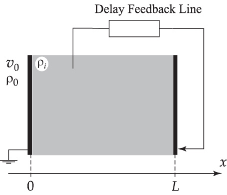
Figure 1: Schematic diagram of Pierce diode with a feedback line

In equations (2)–(5) the non-dimensional variables (space charge potential $\varphi$, density $\rho$, velocity $v$, space coordinate $x$ and time $t$) are used. They are related to the corresponding dimensional variables as follows:

$$\begin{array}[]{c}\varphi^{\prime}=({v^{2}_{0}/\eta})\varphi,\quad E^{\prime}=({v^{2}_{0}/L\eta})E,\\[8.53581pt] \rho^{\prime}=\rho_{0}\rho,\quad v^{\prime}=v_{0}v,\quad x^{\prime}=Lx,\quad t^{\prime}=({L/v_{0}})t,\\ \end{array}$$ (6)

where the dotted symbols correspond to the dimensional values, $\eta$ is the specific electron charge, $v_{0}$ and $\rho_{0}$ are the non-perturbed velocity and density of the electron beam, $L$ is the length of the diode space.

Equations (2) and (3) are numerically integrated with the help of one-step explicit two-level scheme with upstream differences P.J. Rouch (1976); D. Potter (1973); H. Matsumoto, H. Yokoyama, D. Summers (1996) and Poisson equation (4) is solved by the method of the error vector propagation P.J. Rouch (1976). The time and space integration steps have been taken as $\Delta x=0.0005$, and $\Delta t=0.0001$, respectively.

In works B.B. Godfrey (1987); S. Kuhn, A. Ender (1990); H. Matsumoto, H. Yokoyama, D. Summers (1996) it was shown, that in the narrow range $\alpha\sim 3\pi$ without the virtual cathode, one can observe chaotic oscillations in the system. With a decrease of $\alpha$ from $2.88\pi$ to $2.86\pi$ the model demonstrates a transition from periodic oscillations to chaos via a period doubling cascade. Just below the critical value of $\alpha$ the system demonstrates weak chaotic oscillations with the explicit time scale. Below we will call this regime “bond chaos” because the attractor in the reconstructed phase space looks like a narrow bond on which the phase paths are situated. With the further decrease of $\alpha$ the explicit time scale vanishes and the phase picture reminds of spiral twisting from one point. The power spectrum of the system oscillations is more complex in comparison with the first case. This type of chaotic behaviour we call “spiral chaos”.

The stationary homogeneous equilibrium state of the electron beam in Pierce diode is characterized by the following distribution of the system variables

$$\bar{v}(x)=1.0,\quad\bar{\rho}(x)=1.0,\quad\bar{\varphi}(x)=0.0,$$ (7)

that can be found from solutions of stationary equations derived from non-stationary fluid equations (2)–(4) in assumption that $\partial/\partial t=0$.

Homogeneous equilibrium state (7) is stable with $\alpha<\pi$, and loses its stability at $\alpha>\pi$ as it has been shown by J. Pierce J. Pierce (1944). In work A.E. Hramov, I.S. Rempen (2004) the significance of the unstable a decrease of $\alpha$ or with the influence of the external delayed feedback is shown.

II Stabilization of unstable equilibrium spatial state with the help of the continuous delayed feedback

Following the works mentioned above Y.H. Chen, M.Y. Chou (1994); D.J. Gauthier, D.W. Sukow, H.M. Concannon, J.E.S. Socolar (1994); Franz-Josef Elmer (1998); Y.C. Kouomou, P. Woafo (2002); R. Roy, T.W. Murphy, T.D. Maier, Z. Gills, E.R. Hunt (1992); R. Meucci, W. Gadomski, M. Ciofini, F.T. Arecchi (1994); R. Meucci, M. Ciofini, R. Abbate (1996); E. Tziperman, H. Scher, S.E. Zebiak, M.A. Cane (1997); G. Franceschini, S. Bose, E. Schöll (1999) devoted to chaos control in finite-dimensional systems, we now describe the scheme of the continuous delayed feedback for stabilization of the unstable equilibrium state in Pierce diode.

The continuous delayed feedback is realized by changing the potential of the right boundary of the system:

$$\varphi(x=1.0,t)=f_{\rm fb}(t)=K(\rho(x_{\rm fix},t)-\rho(x_{\rm fix},t-d)),$$ (8)

where $K$ is the feedback coefficient, $d$ is the delay time. Variable $\rho(x_{\rm fix},t)$ in (8) is the space charge density in a fixed point $x=x_{\rm fix}$ of diode space (in the work we use $x_{\rm fix}=0.2$). When the stabilization regime takes place and the system is exactly in the equilibrium state, the feedback signal $f_{\rm fb}$ could by compared with the noise level.

Practically, this scheme of delaying feedback can be realized, for example, with the help of delay lines on magnetostatic waves J.D. Gastera (1984); J.C. Sethares (1982) or acoustic waves F. Losee (1997); J. Filipiak, A. Kawalec (1986). Such method would allow to select the required delay time. The signal can be picked out from the system using a probe.

So, unlike works G. Franceschini, S. Bose, E. Schöll (1999); W. Lu, D. Yu, R.G. Harrison (1996); R. Martin, A.J. Scroggie, G.-L. Oppo, W.J. Firth (1996); H. Gang, QuZhilin, (1994); R.O. Grigoriev, M.C. Cross, H.G. Schuster (1997); P. Parmananda, M. Hildebrand, M. Eiswirth (1997); R. Montagne, P. Colet (1997); M.E. Bleich, D. Hochheiser, J.V. Moloney, J.E.S. Socolar (1997); D. Hochheiser, J.V. Moloney, J. Lega (1997), where controlling the chaotic dynamics of the distributed systems needs the effect of the feedback signal upon the whole interaction interval, in our scheme the signal of the continuous delayed feedback determines only the change of the boundary conditions. It is more convenient to realize in experimental microwave devices. Then, in real microwave systems working in the frequency range $0.1\div 100$ GHz, it is nearly impossible to realize the OGY algorithm because it demands very quick changing of controlling parameter.

It must be marked that we use the term continuous feedback in analogy with works K. Pyragas (1992); Y.H. Chen, M.Y. Chou (1994). This term emphasizes that in our scheme the controlling signal is changed continuously in contrast to the schemes based on the OGY algorithm E. Ott, C. Grebogi, J.A. Yorke (1990). It is obvious that the controlling scheme (8) discussed in our work is more convenient in practical use for controlling the dynamics of the distributed microwave systems.

For purpose of stabilization of the unstable equilibrium state the delay time $d$ of the feedback line (8) must be small enough: $d<T_{p}/2$, where $T_{p}=\pi/\omega_{p}$ is the typical time scale in the autonomous distributed system H. Matsumoto, H. Yokoyama, D. Summers (1996).

Results of stabilization of the system (2)–(5) with the help of the continuous feedback (8) are presented in Fig. 2. The autonomous system displays chaotic oscillations with a large amplitude. But after switching on the continuous feedback one can observe a fast decrease of the amplitude of oscillations which leads to the stabilization of the unstable state (7). After a short transient process the controlling signal in the feedback line becomes rather small in comparison with the signal before stabilization (near 0.01%). This means that the regime of chaos control with the help of small controlling signal of continuous feedback takes place in the system.

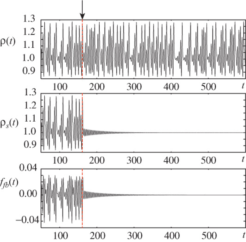
Figure 2: Time series $\rho(x_{\rm fix},t)$ in autonomous system (top picture), oscillations $\rho_{s}(x_{\rm fix},t)$ in stabilized system (middle picture) and the signal in feedback line $f_{\rm fb}(t)$ (bottom picture) for the spiral chaos regime ($\alpha=2.857\pi$). The feedback parameters are $K=0.8$, $d=0.15$. The moment of appearance of the delayed feedback is marked by an arrow and dotted line.

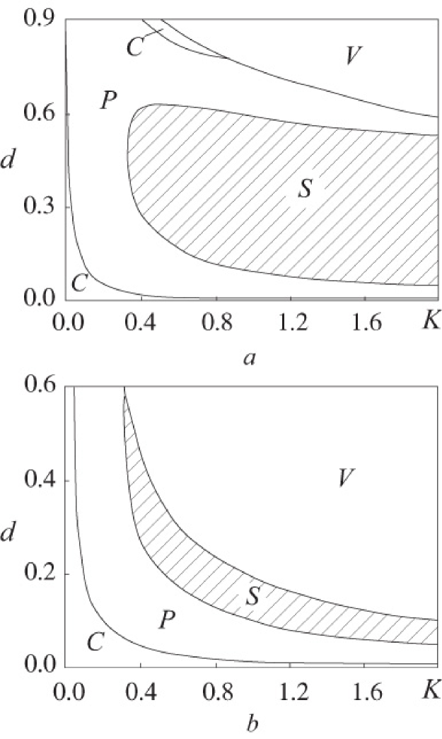
Figure 3: Regime maps of the stabilized system on the plane of parameters $(K,d)$ for cases of (a) bond chaos ($\alpha=2.862\pi$) and (b) spiral chaos ($\alpha=2.857\pi$). The region of stabilization of the unstable equilibrium state is hatched

It is important to find the regions of feedback parameters $K$ and $d$ where chaos controlling is possible. Fig. 3 shows areas of the bond chaos regime ($\alpha=2.862\pi$) and spiral chaos regime ($\alpha=2.857\pi$). One can see that the regime maps ($K,d$) for both cases have qualitative similarities. For small $K$, the system displays chaotic oscillations similar to autonomous oscillations corresponding to this $\alpha$ value (region $C$ in Fig. 3). With an increase of $K$ one can observe the destruction of chaotic oscillations and appearance of periodical ones (region $P$). In this case the feedback signal is not small (its amplitude has the same order of value as $f_{\rm fb}$ before switching on the feedback) hence we can not regard this regime as the controlling chaos one. With further growth of $K$ the controlling chaos regime takes place (region $S$). The unstable homogeneous state is stabilized, and the system dynamics in this case is shown in Fig. 2.

The width of region of stabilization $S$ depends noticeably on the delay time $d$. The threshold values $d_{1}$, $d_{2}$, determine the range $d\in(d_{1},d_{2})$ where controlling parameter values allowing to obtain controlling chaos in the distributed beam-plasma system are possible.

With the further increase of $d$ and $K$, reflection and overtaking of electrons appear in the electron beam (region $V$ in Fig. 3), and therefore the fluid equations (2)–(5) become unfit (see V.N. Shevchik, G.N. Shvedov, A.V. Soboleva (1966); R.F. Soohoo (1971) for detail).

It is useful to note that in spiral chaos regime the region $S$ in the parameter map is narrower than that in bond chaos regime (compare Fig. 3a and 3b).

We can analyse the stability of the discussed equilibrium state by calculating the maximum Lyapunov exponent $\Lambda$ K. Pyragas (1992). For the feedback coefficient $K=0$ the values of Lyapunov exponents of our system are equal to those of the autonomous system.

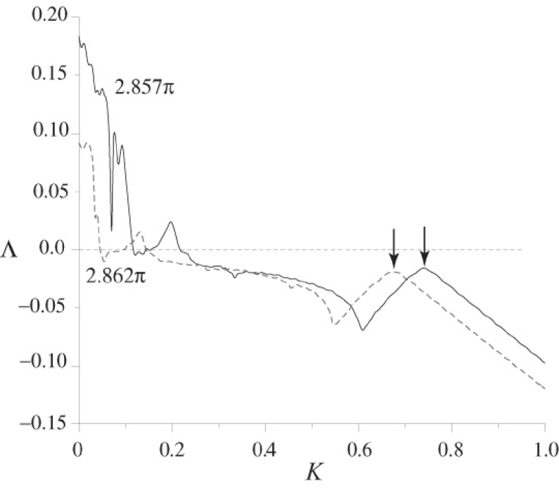
Figure 4: Dependence of the maximum Lyapunov exponent $\Lambda$ upon the feedback coefficient $K$. The dotted line corresponds to the bond chaos regime ($\alpha=2.862\pi$), the solid line — to the spiral chaos regime ($\alpha=2.857\pi$). The arrow marks the values of $K_{c}$, corresponding to the onset of stabilization. $d=0.14$

Fig. 4 shows the dependence between the maximum Lyapunov exponent $\Lambda$ and the feedback coefficient $K$ for two different chaotic regimes. This dependencies determine the boundary of adaptability of our control method. The suppression of the chaotic dynamics is possible only for the values of $K$ corresponding to $\Lambda(K)<0$. These are regions $P$ and $S$ in Fig. 3. The value of $K$ for which stabilization of unstable state takes place (region $S$ in Fig. 3) is marked by an arrow in Fig. 4. One can see that the stabilization regime is preceded by the increase of Lyapunov exponent, and beyond the boundary of stabilization $K=K_{c}$ the value $\Lambda(K)$ decreases linearly. Such behaviour is typical to both types of chaotic dynamics.

III Picking out unstable periodical spatio-temporal states of spatially extended system dynamics

In this section we discuss the unstable periodic spatio-temporal states of distributed active medium, analogous to the unstable periodic orbits of a few-dimensional systems, which play an important role in the complex behavior of non-linear systems P. Cvitanović (1991), in particular, in the case of chaotic synchronization Boccaletti S., Kurths J., Osipov G., Valladares D.L., Zhou C. (2002); Mendoza C., Boccaletti S., Politi A. (2004); Leyva I., Allaria E., Boccaletti S., Arecchi F.T. (2003); Pikovsky A., Zaks M., Rosenblum M., Osipov G., Kurths J. (1997); Pazó D., Zaks M., Kurths J. (2002); Hramov A.E., Koronovskii A.A., Kurovskaya M.K., Moskalenko O.I. (2005).

The initial information about the set of unstable periodic orbits can be obtained from the histograms describing the frequency of system returning to the vicinity of the orbits. This method was offered by D.P. Lathrop E.J. Kostelich D.P. Lathrop, E.J. Kostelich (1989). We choose a phase point ${\bf R}_{i}$ on the attractor. If this point is close to an unstable cycle with a period $T$, then the phase trajectory passing the points ${\bf R}_{i+1}$, ${\bf R}_{i+2}$, …, ${\bf R}_{k}$, will come near the initial state with some precision $\varepsilon>0$:

$$||{\bf R}_{i}-{\bf R}_{i+m}||<\varepsilon,$$ (9)

where $m=T/\Delta t$ is the orbit period in discrete time unit. Then the distribution of return time (histogram) is made. By this histogram it is easy to carry out the typical periods of corresponding unstable states, and then to find the unstable cycles.

For the study of unstable spatio-temporal states of the dynamics of the explored distributed system we investigate the time oscillations of the space charge density $\rho(x_{0},t)$, obtained from the fixed points of the interaction space $x_{0}$. Then, from the time series $\rho(x_{0},t)$, using Takens’ method F. Takens (1981) the attractors of system dynamics are restored in pseudo-phase space $R^{n}$. Using Lathrop & Kostelich algorithm we pick out the periodical orbits in $R^{n}$ and then hence find the spatio-temporal periodical states of the distributed system.

In Fig. 5 the histograms of return time obtained for different values of Pierce parameter are presented. One can see that in the bond chaos regime (Fig. 5) one of the orbits dominate upon the others i.e. it is more frequently visited by phase point.

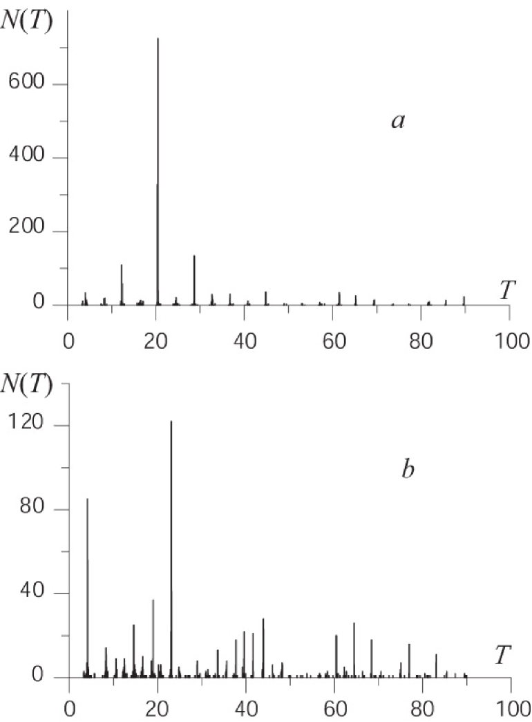
Figure 5: Histograms showing the number of visits of phase trajectory to the fixed attractor points, associated with different recurrence time: (a) $\alpha=2.861\pi$; (b) $\alpha=2.857\pi$

For spiral chaos regime (Fig. 5b) the set of unstable orbits is more complex, and the different unstable periodical states are visited more evenly and frequently.

Histograms of recurrence time obtained for time series $\rho(x,t)$, taken from different points of diode space $x=x_{0}$ are very much alike. This is illustrated in Fig. 6. It follows from the picture that the set of unstable spatio–temporal states is identical along the diode interval. A slight difference can be caused by inaccuracy in calculating the recurrence time (see, for example, the unstable spatio–temporal states with $T=4.173$ in Fig. 6a and Fig. 6c (marked by an arrow)). The latter allows to carry out and to analyse some characteristics of the unstable spatio-temporal states of the distributed system using scalar time series obtained from one fixed point $x_{fix}$ of interaction interval.

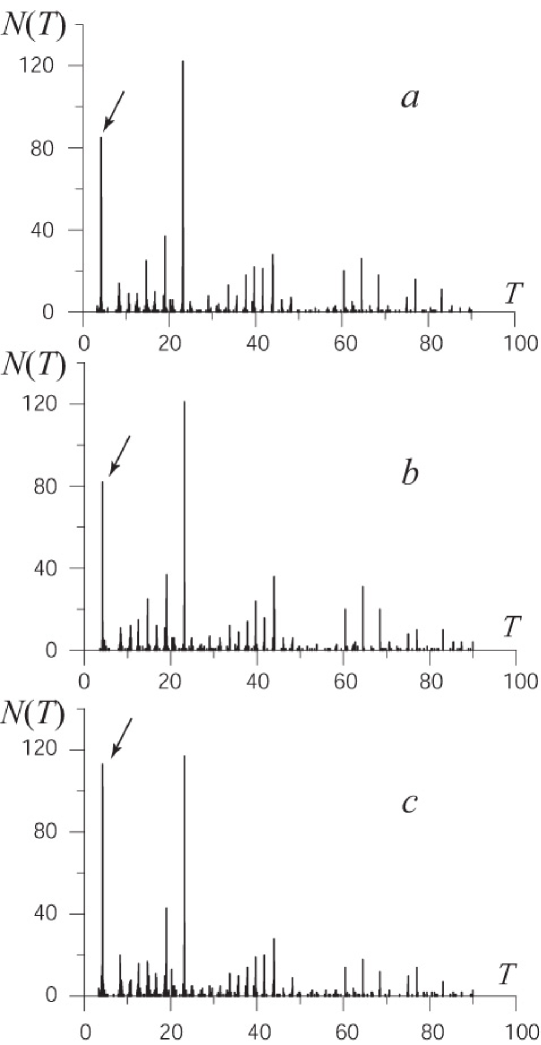
Figure 6: Histograms of recurrence time for $\alpha=2.857\pi$ obtained from the data taken from different points of diode space: (a) $x_{0}=0.2$, (b) $x_{0}=0.5$, (c) $x=0.8$

In Fig. 7 the unstable periodical states of the distributed system are shown. The three-dimensional pictures show the spatio-temporal oscillations of the space charge density $\rho(x,t)$ which correspond to the unstable periodical orbit states with different period. The pictures are obtained for $\alpha=2.857\pi$ (spiral chaos).

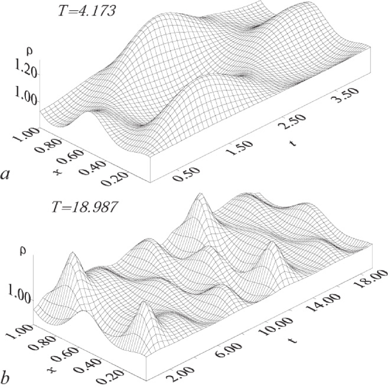
Figure 7: Unstable periodical orbits of different periods $T$ in the regime of spiral chaos: (a) $T=4.173$ and (b) $T=18.987$

We must pay attention that the similar results has been derived when the unstable periodic spatio-temporal states by the method of P. Schmelcher F. Diakonos (SD–method) P. Schmelcher, F.K. Diakonos (1997); D. Pingel, P. Schmelcher, F.K. Diakonos (2001), adapted for the analysis of distributed system. The algorithm is the follows.

As in the case when the unstable periodic states are reconstructed from histograms, at first we determine the system state vector ${\bf R}$ in phase space. As a state vector in this case a vector is taken combined from the density of charge taken from the different points of the interaction space: ${\bf R}(t)=\left\{{\rho(x=0.25,t),\rho(x=0.5,t),\rho(x=0.75,t)}\right\}^{T}$.

In reconstructed phase space a plane $\rho(x=0.25,t)=1.0$ is taken, which is considered as Poincare section. Let us indicate as ${\bf R}_{n}$ the system state corresponding to the $n$th crossing between phase part and the selected section. (this crossing takes place at moment of time $t^{n}$). Then the description of the system can be made with the help of discrete map like

$${\bf R}_{n+1}={\bf G}({\bf R}_{n}),$$ (10)

where ${\bf G}(\cdot)$ is the evolution operator. Obviously, it is impossible to find the analytical form for the operator $\bf G$, but numerical integration of the initial system of fluid equations can give us a consecution of values $\left\{{\bf R}\right\}_{n}$, derived from the map (10).

SD–method for picking out unstable periodic orbits supposes examination of modified model of a distributed system, described by following map D. Pingel, P. Schmelcher, F.K. Diakonos (2001):

$${\bf R}_{n+1}={\bf R}_{n}+\lambda{\bf C}\left[{\bf G}({\bf R}_{n})-{\bf R}_{n}\right].$$ (11)

In the works P. Schmelcher, F.K. Diakonos (1997); D. Pingel, P. Schmelcher, F.K. Diakonos (2001) it is exactly shown that such modified system in the case of analysis of discrete systems and the systems with few degrees of freedom allows to stabilize effectively the unstable periodical orbits of the initial system, which in the case of modified system transform from saddle into stable ones (11). Application of the SD–method to the analysis of distributed system is also effective for picking out unstable periodic spatio-temporal states.

In the equation (11) $\lambda=0.1$ is the method constant and $\bf C$ is a matrix, which, following to work D. Pingel, P. Schmelcher, F.K. Diakonos (2001) was taken as

$${\bf C}=\left(\begin{array}[]{cc}1&0\\ 0&1\\ \end{array}\right).$$ (12)

Modified map (11) allows only to define unstable periodic state of lowest period $T_{1}$, which agrees with the single crossing of the selected Poincare section during time $T_{1}$. To find the unstable states with higher period $T_{p}$, when the phase path crosses the Poincare section for $p$ times during the period $T_{p}$, it is necessary to take a modified map like

$${\bf R}_{n+1}={\bf R}_{n}+\lambda{\bf C}\left[{\bf G}^{p}({\bf R}_{n})-{\bf R}_{n}\right],$$ (13)

where ${\bf G}^{p}(\cdot)$ is $p$ times iterated map ${\bf G}(\cdot)$ (i.e. when numerical solution of the system of fluid equations is found and then the map is reconstructed (13) it is necessary to take into account only the every $p$th crossing of the Poincare section by phase path, where $p$ is obviously integer.

So, by numerical integration of the map (13) with different values of $p$ one can find the unstable spatio-temporal states that appear to be stable in the modified system, described by the map (13). So, the result of numerical integration of modified system (fluid equations taking into account the procedure (13))) is a periodic solution, which agrees with the unstable periodic state of the initial system.

The numerical integration of the modified system causes only one difficulty. When we are searching for the state ${\bf R}_{n+1}$ at the moment $t^{n+1}$, then, according to formula (13) we know only the coordinates of this state in Poincare section but we don’t know the corresponding distribution of space charge density $\rho(x,t^{n+1})$, velocity $v(x,t^{n+1})$ of the electron beam and the potential $\phi(x,t^{n+1})$. To derive the mentioned space functions we use the following procedure. The system of fluid equations describing Pierce diode is integrated till some state ${\bf R}_{s}$ of the system would not be close to the selected state ${\bf R}_{n+1}$ with some demanded precision: $||{\bf R}_{n+1}-{\bf R}_{s}||<\delta$, where $\delta$ is taken as $\delta=10^{-3}$. When this condition is fulfilled, the space functions corresponding to the state ${\bf R}_{s}$ are considered as the space distributions ${\bf R}_{n+1}$ and then the next iteration according to (13) takes place.

As numerical modelling shows, the modified SD–method applied to distributed system is convergent and allows to find the demanded periodical time-space states. The convergence of the procedure is illustrated by Fig. 8, which shows the dependance of the space charge density $\rho(x=0.25)$ in the moment when the point in pseudo-phase space crosses the Poincare section upon the number of iteration $n$ of the SD–method when the unstable state of period 1 is defined ($p=1$). One can see clearly that the iteration process of SD–method converges to the value corresponding to the unstable time-periodical spatio-temporal state of the system. Fig. 9 shows the time series of $\rho(t,x=0.2)$, corresponding to unstable periodic states of different order $p$ and period $T$ with $\alpha=2.858\pi$, picked by SD–method. We mark that the derived spatio-temporal distributions agrees very well with the distributions of unstable states derived earlier by analysing of the return time histograms.

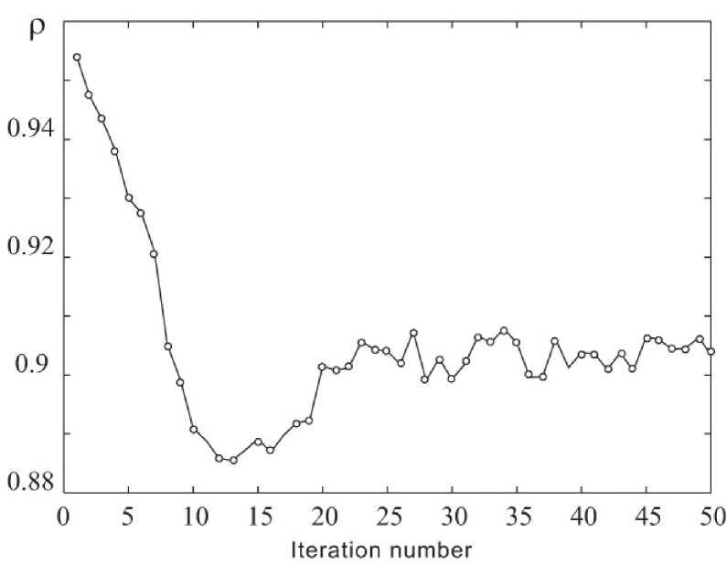
Figure 8: Dependance of the space charge density $\rho$ taken at the moment when the phase point passes the Poincare section, upon the number of iteration of SD–method when the orbit of period 1 ($T=4.2$) is picked out. Pierce parameter $\alpha=2.858\pi$

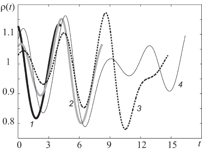
Figure 9: Time series of the space charge density $\rho(t)$ in the fixed point of the phase space $x=0.2$, corresponding to the different unstable periodic spatio-temporal states picked out by SD–method with $\alpha=2.858\pi$: 1 – $T=4.2$ ($p=1$), 2 – $T=9.1$ ($p=2$), 3 – $T=16.9$ ($p=3$), 1 – $T=18.9$ ($p=4$)

As quantitative characteristics of the derived unstable orbits it is useful to analyze the maximum Lyapunov exponent $\Lambda$ of every orbit. Calculation of this value is important for further stabilization of periodical spatio-temporal states.

Values of maximum Lyapunov exponent $\Lambda^{T}$ calculated with the help of Benettin’s algorithm G. Benettin, L. Galgani, J.-M. Strelcyn (1976) for the most frequently visited orbits are presented in Table 1.

Table. 1: Values of maximum Lyapunov exponent $\Lambda^{T}$ for unstable states with period $T$ in the regime of spiral chaos ($\alpha=2.857\pi$)

Period of unstable	Maximum Lyapunov
state $T$	exponent $\Lambda^{T}$
4.347	0.854
8.289	1.194
10.581	0.698
12.501	0.629
14.613	0.337
18.987	0.266
23.115	0.186
39.636	0.094
43.953	0.083
60.438	0.053

IV Stabilization of the unstable periodical states

As simplest scheme of stabilization of unstable periodical orbits described in the previous section, we can take the scheme (8) where the feedback signal is formed as:

$$\varphi(x=1.0,t)=f^{T}_{\rm fb}(t)=$$

$$=K(\rho(x_{\rm fix},t)-\rho(x_{\rm fix},t-T_{k}))=K\xi(t).$$ (14)

Here $K$ is again the feedback coefficient and $T_{k}$ is the delay time equal to the period of the $k$-th unstable orbit. As in the case of stabilization of unstable equilibrium state, we choose the fixed point of the diode space $x_{\rm fix}=0.2$, from which the feedback signal is taken.

The numerical modelling shows that this scheme is rather effective for stabilization of the unstable periodical state with the lowest period $T_{1}$. Fig. 10 shows the spatio–temporal dynamics of the system in cases of autonomous oscillations and in the regime of stabilization (the value of the space charge density $\rho(x,t)$ is shown by colour nuances scaling). One can easily observe that there are peculiarities of the complex spatio-temporal behaviour and transitions between chaotic and periodic regimes. It is obvious from the picture that the periodic dynamics analogous to the system behaviour near the unstable state is stabilized during approximately $2\div 3$ time periods $T_{1}$ (see Fig. 7a).

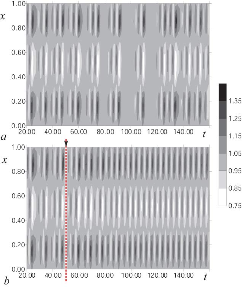
Figure 10: Spatio–temporal dynamics of Pierce diode in chaotic regime (a) and in the regime of stabilization of the periodic orbit $T=4.173$ (b). The arrow and dotted line in  b shows the moment of switching on the delayed feedback

We also study the peculiarities of the influence of delayed feedback (14) upon the investigated system by examining how the feedback amplitude $K$ acts upon the maximum Lyapunov exponent $\Lambda$ and the average of the feedback signal

$$\langle{\xi}\rangle=\frac{1}{\tau}\int_{0}^{\tau}f^{T}_{\rm fb}(t)\,dt,$$ (15)

where $\tau\gg d$. The corresponding plots derived for $d=T_{1}$ are presented in Fig. 11.

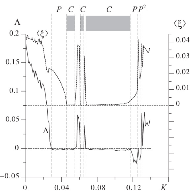
Figure 11: Dependence of the maximum Lyapunov exponent (solid line) and the mean feedback signal (doted line) upon the feedback coefficient $K$ in the spiral chaos regime ($\alpha=2.857\pi$). Region $C$ (grey colour) corresponds to the regime of stabilization of the unstable periodic state of period 1 $T=4.173$ (the feedback signal is close to null $\langle{\xi}\rangle\approx 0$). Region $P$ corresponds to periodic oscillations, when the feedback signal is large and the maximum Lyapunov exponent $\Lambda<0$; region $P^{2}$ corresponds to the regime of period doubling

When $K$ is small the system demonstrates chaotic oscillations similar to the oscillations in the autonomous regime (in Fig. 12a, one can see the time series of the space charge oscillations for $x=0.2$ without feedback). With an increase of $K$ the complexity of the oscillations diminishes (the value of $\Lambda$ decreases) and at the same time the amplitude of the feedback signal becomes smaller. In some region of $K$ the feedback signal is close to zero and the maximum Lyapunov exponent $\Lambda<0$ (the grey area in Fig. 11). In this case the spatio-temporal dynamics is the same as that of the unstable periodic state. Thus, it is the regime of chaos stabilization, illustrated by Fig. 12b,c, which shows the oscillations of the space charge density in the system and the feedback signal, correspondingly.

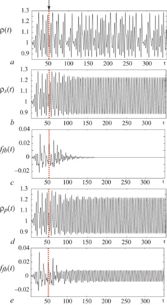
Figure 12: Time series $\rho(x_{\rm fix},t)$ of the autonomous system (a), time series $\rho_{s}(x_{\rm fix},t)$ in the stabilized system ($K=0.07$, $d=T=4.173$) (b), feedback signal $f_{\rm fb}(t)$ (c); time series $\rho_{p}(x_{\rm fix},t)$ and $f_{\rm fb}(t)$ (d,e) in periodic oscillation regime ($\Lambda<0$) ($K=0.035$, $d=T=4.173$), $\alpha=2.857\pi$ (spiral chaos regime). The moment of switching on the feedback is marked by an arrow and a dotted line.

Examining the graph $\Lambda(K)$ we also must note the regions where the feedback signal $\langle{\xi}\rangle$ is not small but the value $\Lambda<0$. These regimes are marked in Fig. 11 as $P$ and correspond to periodic oscillations near the unstable orbit. The space charge oscillations and the feedback signal for this case are presented in Fig. 12d,e. We also pay attention to the fact, that with large $K$ the system demonstrates the period doubling based on the regime $P$ (region marked as $P^{2}$ in Fig. 11). For $K>0.15$ in the system the growth of the oscillation amplitude takes place, and reflection of electrons appears. Thus, in this region we can not use any more the fluid equations for the description of the system V.N. Shevchik, G.N. Shvedov, A.V. Soboleva (1966); R.F. Soohoo (1971).

But the computer experiment shows that stabilization of the unstable orbits with higher periods $T_{k}>T_{1}=4.173$ using feedback scheme (14) is impossible. The analysis of the chaos controlling schemes like (14) applied to the systems with few degrees of freedom, has shown W. Just (1999) that the effective stabilization of the unstable periodic orbits is possible only when the values of the maximum Lyapunov exponent $\lambda$ and the orbit period $\tau$ fulfill the following condition

$$\lambda\tau\leq C,$$ (16)

where $C$ is constant depending on the system.

Thus, we must modify the controlling scheme (14) so that it would be possible to stabilize the orbits with higher period $T_{k}$. The scheme, which we consider, is a modification of the method worked out by K. Pyragas K. Pyragas (1992). As it follows from the result of the numerical experiment J.E.S. Socolar, D.W. Sukow, D.J. Gauthier (1994), in the few-dimensional non-linear systems this scheme allows to stabilize the unstable orbits for which the condition (16) does not fulfill. The main idea of the method J.E.S. Socolar, D.W. Sukow, D.J. Gauthier (1994) is the following: the feedback signal is formed so that not only the system state at the moment $(t-T_{k})$ influences upon it, as it was in the previous scheme, but also the states at the moments of time $(t-mT_{k})$ do, with some weight coefficients. Following work G. Franceschini, S. Bose, E. Schöll (1999), we assume that the described scheme could be effective in the controlling dynamics of the distributed chaotic system.

The continuous feedback for stabilization of the unstable periodic states of higher period $T_{k}>T_{1}$ can be described by the following expression

$$\varphi(x=1.0,t)=K\xi(t)=$$

$$=K\left((1-r)\sum\limits_{m=1}^{M}r^{m-1}\left(\rho(x_{\rm fix},t)-\rho(x_{\rm fix},t-md)\right)\right),$$ (17)

where the delay time $d$ is taken equal to the period of the stabilized periodic orbit $T_{k}$, $M$ is large enough ($M\gg 1$), and $r$ ($0\leq r<1$) characterizes the contribution of the previous system’s states into the feedback signal: small values of $r$ correspond to the small significance of the previous states in the signal (17), and analogously, correspond to the large ones. The case $r=0$ corresponds to the simplest scheme (14) of continuous feedback discussed above. Such feedback scheme (17) can be realized in practice, for example, by using a set of acoustic time delay lines each with its own delay time and transfer constant. As it follows from works G. Franceschini, S. Bose, E. Schöll (1999); M.E. Bleich, J.E.S. Socolar (1999); C. Simmendinger, D. Preiber, O.G. Hess (1999), a possibility of stabilization of the orbits of highest period $T_{k}$ (16) appears with the growth of $r$, for which the use of the scheme (14) is impossible. For example, in the work W. Just (1999) it is shown that with the help of the scheme similar to (17) it is possible to stabilize the unstable periodic states for which the following estimation condition is fulfilled:

$$\Lambda T\leq C\frac{1+r}{1-r}.$$ (18)

Using the scheme (17) for the stabilization of the periodic orbits which fulfills the condition (18), the explicit knowledge of the orbit period $T_{k}$ is needed. If the delay time $d$ differs even slightly from the real period $T_{k}$, it is impossible to stabilize the unstable periodic state of the system, and in the feedback line one can observe periodic oscillations $\xi(t)$ with the amplitude exceeding significantly the noise level in the system. As numerical analysis shows, stabilization is possible only when the orbit period is known with the precision $\varepsilon<0.01\%$.

For more accurate definition of the orbit periods $T_{k}$ the following method presented in work A. Kittel, J. Parisi, K. Pyragas (1995) for the systems with few degrees of freedom and approbated for distributed systems in the work G. Franceschini, S. Bose, E. Schöll (1999) is used.

If the delay time $d$ is not explicitly “tuned” to the orbit period $T_{k}$ then the maximum Lyapunov exponent is negative and in the feedback line one can observe the oscillations with the amplitude exceeding significantly the noise level of the system and the “base” period $\Theta\not=T_{k}$, which depends upon $K$ and $d$ (see. Fig. 12d,e). In work W. Just (1999) the analytical dependence between the unknown explicit period $T_{k}$ of the unstable state, feedback parameters $K$, $d$ and the period $\Theta$ has been found as follows:

$$\Theta(K,d)=T_{k}+\frac{K}{K-g}(d-T_{k})+{\rm O}({(d-T)^{2}}).$$ (19)

Here $g$ is the unknown parameter which is defined by the type of the non-linear dynamical system and depends on the form of the delayed feedback. Thus, in expression (19) there are two unknown values: the period $T_{k}$ of the unstable periodic state and the parameter $g$.

Let us take two sets of values $(K_{1},d_{1})$, $(K_{2},d_{2})$, where the values of $d_{1,2}$ are chosen close to the period of the stabilized orbit, and then find the corresponding $\Theta_{1}$ and $\Theta_{2}$. Then we find numerically the solution of the system of two non-linear equations (19) and determine the values $g$ and $T_{k}$. Then we repeat the procedure taking the newly defined $T_{k}$ as $d$. After a number of such iterations the period of the unstable orbit $T_{k}$, would be defined with absolutely satisfactory precision and then the scheme (17) could be used for stabilization of this state.

Numerical analysis shows that with the help of this method it is possible to stabilize the orbits with the period $T<25.0$. The unstable states with higher period turned out to be impossible to stabilize, though in the system the periodic oscillations can be observed, but the form of these oscillations is not close to the concerned unstable state and the feedback signal is not small. With the growth of the period $T$ of the stabilized orbit it was necessary to enlarge the parameters $M$ and $r$ to achieve the effect of controlling chaos. Simultaneously, the range of value of the feedback coefficient $K$, for which stabilization of the unstable state is possible, narrows.

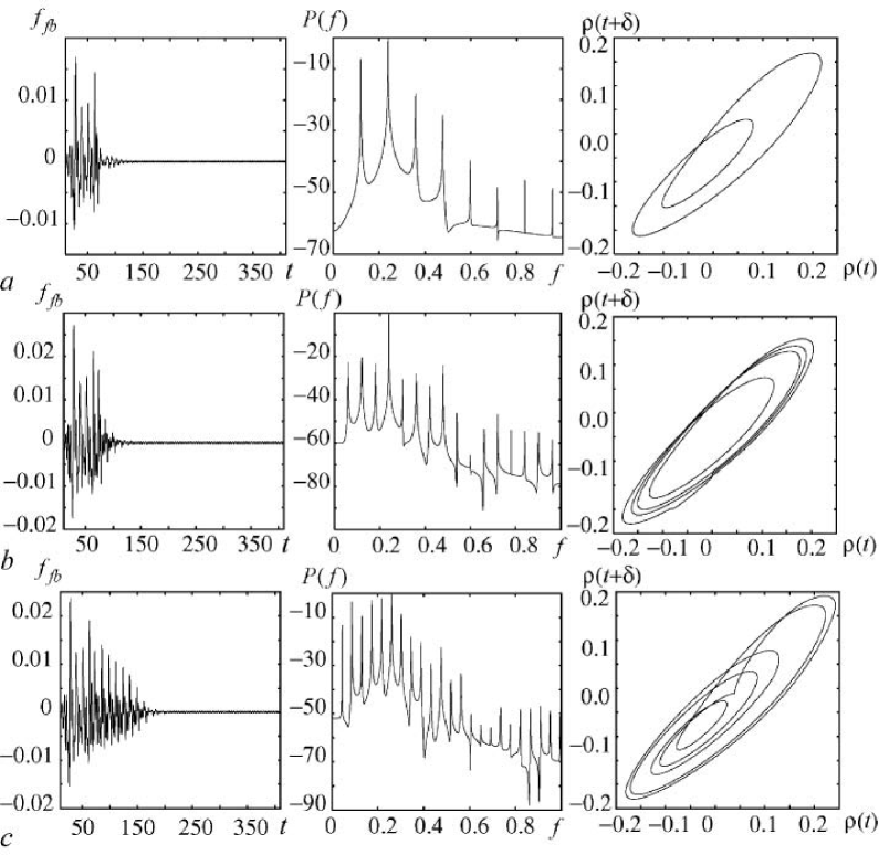
Figure 13: Stabilization of the unstable states of high period: (a) $T=8.3829$ ($M=3$, $K=0.03$, $r=0.2$); (b) $T=16.6582$ ($M=12$, $K=0.012$, $r=0.38$); (c) $T=23.1286$ ($M=20$, $K=0.008$, $r=0.56$). The pictures (from left to right) present: the time series of feedback signal $f_{\rm fb}$, the power spectrum of the oscillations in stabilized system and the phase portrait for the space charge density oscillations $\rho(x_{\rm fix}=0.2,t)$. The feedback is switched on at the moment of time $t=50.0$. Delay time of time-delayed embedding $\delta=1$

Stabilization of the orbits of highest period is illustrated by Fig. 13. The feedback scheme parameters $M$, $r$ and $K$ are defined in the cutline. The explicit values of the periods $T$ are defined according to the method described above. In Fig. 13 the orbits of the period $T\approx 8$, $T\approx 16$ and $T\approx 23$ are shown. The latter is the unstable orbit with the highest period which appears to be possible to stabilize in spiral chaos regime ($\alpha=2.857\pi$) with the help of the discussed scheme.

Conclusion

In this work the method of controlling complex chaotic dynamics of the spatially distributed active medium “electron beam with overcritical current in Pierce diode” is discussed. The described method is based on the ideas of controlling chaos in non-linear systems with few degrees of freedom. The scheme of continuous delayed feedback, which is used for controlling, allows to stabilize the unstable equilibrium state of the distributed system and the unstable periodic spatio–temporal states analogous to the unstable periodic orbits of the chaotic attractor in the systems with few degrees of freedom.

References

- E. Ott, C. Grebogi, J.A. Yorke (1990) E. Ott, C. Grebogi, J.A. Yorke, Phys. Rev. Lett. 64, 1196 (1990).
- S. Boccaletti, C. Grebogi, Y.-C. Lai, H. Mancini, D. Maza (2000) S. Boccaletti, C. Grebogi, Y.-C. Lai, H. Mancini, D. Maza, Physics Reports 329, 103 (2000).
- C. Grebogi, E. Ott, J.A. Yorke (1988) C. Grebogi, E. Ott, J.A. Yorke, Phys. Rev. A 37, 1711 (1988).
- D.P. Lathrop, E.J. Kostelich (1989) D.P. Lathrop, E.J. Kostelich, Phys. Rev. A 40, 4028 (1989).
- P. Schmelcher, F.K. Diakonos (1997) P. Schmelcher, F.K. Diakonos, Phys. Rev. Lett. 78, 4733 (1997).
- M. Dhamala, Y.-Ch. Lai (1999) M. Dhamala, Y.-Ch. Lai, Phys. Rev. E 60, 6176 (1999).
- T.L. Carroll (1999) T.L. Carroll, Phys. Rev. E 59, 1615 (1999).
- J.A.C. Gallas (2001) J.A.C. Gallas, Phys. Rev. E 63, 016216 (2001).
- D. Pingel, P. Schmelcher, F.K. Diakonos (2001) D. Pingel, P. Schmelcher, F.K. Diakonos, Phys. Rev. E 64, 026214 (2001).
- W.L. Ditto, S.N. Rauseo, M.L. Spano (1990) W.L. Ditto, S.N. Rauseo, M.L. Spano, Phys. Rev. Lett. 65, 3211 (1990).
- E.R. Hunt (1991) E.R. Hunt, Phys. Rev. Lett. 67, 1953 (1991).
- S. Bielawski, D. Derozier, P. Glorieux (1993) S. Bielawski, D. Derozier, P. Glorieux, Phys. Rev. A 47, R2492 (1993).
- T. Shinbrot, E. Ott, C. Grebogi, J.A. Yorke (1993) T. Shinbrot, E. Ott, C. Grebogi, J.A. Yorke, Nature 363, 411 (1993).
- M. Ding, W. Yang, V. In, W.L. Ditto (1996) M. Ding, W. Yang, V. In, W.L. Ditto, Phys. Rev. E. 53, 4334 (1996).
- K. Pyragas (1992) K. Pyragas, Phys. Lett. A 170, 421 (1992).
- Y.H. Chen, M.Y. Chou (1994) Y.H. Chen, M.Y. Chou, Phys. Rev. E. 50, 2331 (1994).
- D.J. Gauthier, D.W. Sukow, H.M. Concannon, J.E.S. Socolar (1994) D.J. Gauthier, D.W. Sukow, H.M. Concannon, J.E.S. Socolar, Phys. Rev. E. 50, 2343 (1994).
- Franz-Josef Elmer (1998) Franz-Josef Elmer, Phys. Rev. E. 57, R4903 (1998).
- Y.C. Kouomou, P. Woafo (2002) Y.C. Kouomou, P. Woafo, Phys. Rev. E 66, 036205 (2002).
- R. Roy, T.W. Murphy, T.D. Maier, Z. Gills, E.R. Hunt (1992) R. Roy, T.W. Murphy, T.D. Maier, Z. Gills, E.R. Hunt, Phys. Rev. Lett. 68, 1259 (1992).
- R. Meucci, W. Gadomski, M. Ciofini, F.T. Arecchi (1994) R. Meucci, W. Gadomski, M. Ciofini, F.T. Arecchi, Phys. Rev. E 49, R2528 (1994).
- R. Meucci, M. Ciofini, R. Abbate (1996) R. Meucci, M. Ciofini, R. Abbate, Phys. Rev. E 53, R5537–R5540 (1996).
- E. Tziperman, H. Scher, S.E. Zebiak, M.A. Cane (1997) E. Tziperman, H. Scher, S.E. Zebiak, M.A. Cane, Phys. Rev. Lett. 79, 1034 (1997).
- G. Franceschini, S. Bose, E. Schöll (1999) G. Franceschini, S. Bose, E. Schöll, Phys. Rev. E. 60, 5426 (1999).
- W. Lu, D. Yu, R.G. Harrison (1996) W. Lu, D. Yu, R.G. Harrison, Phys. Rev. Lett. 76, 3316 (1996).
- R. Martin, A.J. Scroggie, G.-L. Oppo, W.J. Firth (1996) R. Martin, A.J. Scroggie, G.-L. Oppo, W.J. Firth, Phys. Rev. Lett. 77, 4007 (1996).
- H. Gang, QuZhilin, (1994) H. Gang, QuZhilin,, Phys. Rev. Lett. 72, 68 (1994).
- R.O. Grigoriev, M.C. Cross, H.G. Schuster (1997) R.O. Grigoriev, M.C. Cross, H.G. Schuster, Phys. Rev. Lett. 79, 2795 (1997).
- P. Parmananda, M. Hildebrand, M. Eiswirth (1997) P. Parmananda, M. Hildebrand, M. Eiswirth, Phys. Rev. E 56, 239 (1997).
- R. Montagne, P. Colet (1997) R. Montagne, P. Colet, Phys. Rev. E 56, 4017 (1997).
- S. Boccaletti, J. Bragard, F.T. Arecchi (1999) S. Boccaletti, J. Bragard, F.T. Arecchi, Phys. Rev. E. 59, 6574 (1999).
- M.E. Bleich, D. Hochheiser, J.V. Moloney, J.E.S. Socolar (1997) M.E. Bleich, D. Hochheiser, J.V. Moloney, J.E.S. Socolar, Phys. Rev. E 55, 2119 (1997).
- D. Hochheiser, J.V. Moloney, J. Lega (1997) D. Hochheiser, J.V. Moloney, J. Lega, Phys. Rev. A 55, R4011 (1997).
- N. Krahnstover et al (1998) N. Krahnstover et al, Phys. Lett. A 239, 103 (1998).
- H. Friedel, R. Grauer, H.K. Spatschek (1998) H. Friedel, R. Grauer, H.K. Spatschek, Physics of plasmas 5, 3187 (1998).
- J. Pierce (1944) J. Pierce, J.Appl.Phys. 15, 721 (1944).
- H. Matsumoto, H. Yokoyama, D. Summers (1996) H. Matsumoto, H. Yokoyama, D. Summers, Phys.Plasmas 3, 177 (1996).
- A.E. Hramov, I.S. Rempen (2004) A.E. Hramov, I.S. Rempen, Int. J.Electronics 91, 1 (2004).
- A.V. Mamaev, M. Saffman (1998) A.V. Mamaev, M. Saffman, Phys. Rev. Lett. 80, 3499 (1998).
- L. Pastur, L. Gostiaux, U. Bortolozzo, S. Boccaletti, P.L. Ramazza (2004) L. Pastur, L. Gostiaux, U. Bortolozzo, S. Boccaletti, P.L. Ramazza, Phys. Rev. Lett. 93, 063902 (2004).
- F. T. Arecchi, S. Boccaletti, P. L. Ramazza, and S. Residori (2004) F. T. Arecchi, S. Boccaletti, P. L. Ramazza, and S. Residori, Phys. Rev. Lett. 70, 2277 (1993).
- B.B. Godfrey (1987) B.B. Godfrey, Phys. Fluids 30, 1553 (1987).
- S. Kuhn, A. Ender (1990) S. Kuhn, A. Ender, J.Appl.Phys. 68, 732 (1990).
- P.A. Lindsay, X. Chen, M. Xu (1995) P.A. Lindsay, X. Chen, M. Xu, Int. J.Electronics 79, 237 (1995).
- P.J. Rouch (1976) P.J. Rouch, Computational fluid dynamics (Hermosa publishers, Albuquerque, 1976).
- D. Potter (1973) D. Potter, Computational physics (John Wiley & Sons Ltd., 1973).
- J.C. Sethares (1982) J.C. Sethares, J.Appl.Phys 53, 2646 (1982).
- J.D. Gastera (1984) J.D. Gastera, J.Appl.Phys 55, 2506 (1984).
- F. Losee (1997) F. Losee, RF Systems, Components, and Circuits Handbook (Artech House, 1997).
- J. Filipiak, A. Kawalec (1986) J. Filipiak, A. Kawalec, Electr. Lett. 22, 976 (1986).
- V.N. Shevchik, G.N. Shvedov, A.V. Soboleva (1966) V.N. Shevchik, G.N. Shvedov, A.V. Soboleva, Wave and Oscillatory Phenomena in Electron Beams at Microwave Frequencies (Pergamon Press, Oxford, 1966).
- R.F. Soohoo (1971) R.F. Soohoo, Microwave Electronics (Addison-Wesley Longman, 1971).
- P. Cvitanović (1991) P. Cvitanović, Physica D 51, 138 (1991).
- Boccaletti S., Kurths J., Osipov G., Valladares D.L., Zhou C. (2002) Boccaletti S., Kurths J., Osipov G., Valladares D.L., Zhou C., Physics Reports 366, 1 (2002).
- Mendoza C., Boccaletti S., Politi A. (2004) Mendoza C., Boccaletti S., Politi A., Phys. Rev. E. 69, 047202 (2004).
- Leyva I., Allaria E., Boccaletti S., Arecchi F.T. (2003) Leyva I., Allaria E., Boccaletti S., Arecchi F.T., Phys. Rev. E. 68, 066209 (2003).
- Pikovsky A., Zaks M., Rosenblum M., Osipov G., Kurths J. (1997) Pikovsky A., Zaks M., Rosenblum M., Osipov G., Kurths J., Chaos 7, 680 (1997).
- Pazó D., Zaks M., Kurths J. (2002) Pazó D., Zaks M., Kurths J., Chaos 13, 309 (2002).
- Hramov A.E., Koronovskii A.A., Kurovskaya M.K., Moskalenko O.I. (2005) Hramov A.E., Koronovskii A.A., Kurovskaya M.K., Moskalenko O.I., Phys. Rev. E 71, 056204 (2005).
- F. Takens (1981) F. Takens, in Lectures Notes in Mathematics, edited by Rand D., Young L.–S (N.Y.: Springler–Verlag, 1981), p. 366.
- G. Benettin, L. Galgani, J.-M. Strelcyn (1976) G. Benettin, L. Galgani, J.-M. Strelcyn, Phys. Rev. A14, 2338 (1976).
- W. Just (1999) W. Just, in Handbook of Chaos Control, edited by H.G. Schuster (Weinheim: Wiley-VCH, 1999).
- J.E.S. Socolar, D.W. Sukow, D.J. Gauthier (1994) J.E.S. Socolar, D.W. Sukow, D.J. Gauthier, Phys. Rev. E 50, 3245 (1994).
- M.E. Bleich, J.E.S. Socolar (1999) M.E. Bleich, J.E.S. Socolar, Phys. Lett. A 210, 87 (1999).
- C. Simmendinger, D. Preiber, O.G. Hess (1999) C. Simmendinger, D. Preiber, O.G. Hess, Optics Express 5, 48 (1999).
- A. Kittel, J. Parisi, K. Pyragas (1995) A. Kittel, J. Parisi, K. Pyragas, Phys. Lett. A 198, 433 (1995).