Numerical simulations of current generation and dynamo excitation in a mechanically-forced, turbulent flow

Abstract

The role of turbulence in current generation and self-excitation of magnetic fields has been studied in the geometry of a mechanically-driven, spherical dynamo experiment, using a three dimensional numerical computation. A simple impeller model drives a flow which can generate a growing magnetic field, depending upon the magnetic Reynolds number $Rm=\mu_{0}\sigma Va$ and the fluid Reynolds number $Re=Va/\nu$ of the flow. For $Re<420$ the flow is laminar and the dynamo transition is governed by a simple threshold in $Rm>100$, above which a growing magnetic eigenmode is observed that is primarily of a dipole field tranverse to axis of symmetry of the flow. In saturation the Lorentz force slows the flow such that the magnetic eigenmode becomes marginally stable. For $Re>420$ and $Rm\sim 100$ the flow becomes turbulent and the dynamo eigenmode is suppressed. The mechanism of suppression is due to a combination of a time varying large-scale field and the presence of fluctuation driven currents (such as those predicted by the mean-field theory) which effectively enhance the magnetic diffusivity. For higher $Rm$ a dynamo reappears, however the structure of the magnetic field is often different from the laminar dynamo; it is dominated by a dipolar magnetic field aligned with the axis of symmetry of the mean-flow which is apparently generated by fluctuation-driven currents. The magnitude and structure of the fluctuation-driven currents has been studied by applying a weak, axisymmetric seed magnetic field to laminar and turbulent flows. An Ohm’s law analysis of the axisymmetric currents allows the fluctuation-driven currents to be identified. The magnetic fields generated by the fluctuations are significant: a dipole moment aligned with the symmetry axis of the mean-flow is generated similar to those observed in the experiment, and both toroidal and poloidal flux expulsion are observed.

I Introduction

Astrophysical and geophysical magnetic fields are generated by complex flows of plasmas or conducting fluids which convert gravitational potential, thermal, and rotational energies into magnetic energy moffatt78 ; childress95 . A comprehensive theory of the magnetohydrodynamic dynamo is elusive since the generating mechanism can vary dramatically from one system to another. These variations arise from differences in free energy sources, conductivity and viscosity of the conducting media, and geometry. Isolating and understanding the mechanisms by which self-generation occurs and the role of turbulence in the transition to a dynamo remain important problems.

Dynamo action arises from the electromotive force (EMF) induced by the movement of an electrically-conducting medium through a magnetic field. This motional EMF generates a magnetic field which, depending on the details of the motion, can either amplify or attenuate the initial magnetic field. If the induced field reinforces the initial magnetic field, then the positive feedback leads to a growing magnetic field. The source of energy for this dynamo is the kinetic energy of the moving fluid. The fluid may be driven by many different mechanisms such as thermal convection in a rotating body for the case of the Earth, or by impellers in liquid sodium dynamo experiments.

When the system is turbulent, the turbulence likely plays an important role in the dynamo onset and the saturated state. In the saturated state, the backreaction of the self-generated magnetic field modifies the velocity field. It is well known that in hydrodynamics, turbulence converts large-scale motions into smaller and smaller eddies, a process known as a turbulent cascade. In magnetohydrodynamics (MHD), fluid turbulence can fold a large-scale magnetic field into smaller structures kraichnan67 . If the small-scale magnetic fluctuations are helical, they can, on average, generate a net EMF by interacting with the velocity field fluctuations and drive large-scale currents. When the magnetic field of this fluctuation driven current reinforces the original magnetic field self-excitation may be possible. Thus the generation of small-scale currents may explain observed large-scale magnetic fields frisch75 ; pouquet78 ; alexakis05 .

Exact treatment of current generation in electrically-conducting fluids requires solving the MHD equations governing the magnetic and velocity fields:

$$\frac{\partial\bm{\mathrm{B}}}{\partial t} = \frac{1}{\mu_{0}\sigma}\nabla^{2}\bm{\mathrm{B}}+\bm{\nabla}\times\bm{\mathrm{v}}\times\bm{\mathrm{B}}$$ (1)

$$\rho\left[\frac{\partial\bm{\mathrm{v}}}{\partial t}+\left(\bm{\mathrm{v}}\cdot\bm{\nabla}\right)\bm{\mathrm{v}}\right] = \bm{\mathrm{J}}\times\bm{\mathrm{B}}+\rho\nu\bm{\nabla}^{2}\bm{\mathrm{v}}-\bm{\nabla}{\it p}+\bm{\mathrm{F}}$$ (2)

where $\rho$ is the density, $\sigma$ is the conductivity, $\nu$ is the viscosity, and $p$ is the pressure. ${\bf F}$ is a driving term annotating the sundary sources of free energy in the flow. Eqs. 1 and 2 are highly nonlinear and, without limiting assumptions, are analytically intractable. Early dynamo theory focused on solving only Eq. 1 in the kinematic limit where the linear magnetic field stability of prescribed velocity fields was calculated to determine whether magnetic field growth was possible bullard54 ; roberts72 ; gubbins73 . Due to advances in computing power during the last decade, great progress has been made by performing numerical simulations of dynamos, which simultaneously solve the non-linear MHD equations (Eqs. 1 and 2). These studies break into two separate classes: global simulations which attempt to model geophysical or astrophysical dynamos such as the Earth and the Sun glatzmaier84 ; glatzmaier95 ; glatzmaier02 ; kageyama95 ; kageyama97 ; kuang97 , and simplified models in which the geometry is simple enough to uniquely identify particular physical effects meneguzzi81 ; cattaneo96 ; mueller03 .

The numerical simulations have been useful for studying magnetic field generation, even though they are still far away from being able to resolve the fluid turbulence of the actual systems. In particular, the role of the magnetic Prandtl number, $Pm=Rm/Re$, on threshold conditions for magnetic field growth is of importance for understanding magnetic field generation in the Earth, Sun, and in experiments. The linear self-excitation of the magnetic field is governed by the magnetic Reynolds number, $Rm=\mu_{0}\sigma LV_{0}$, where $\sigma$ is the molecular electrical conductivity, $L$ is a characteristic size of the conducting region, and $V_{0}$ is the peak speed. Hydrodynamic turbulence is governed by the fluid Reynolds, number $Re=V_{0}\ell/\nu$, where $\ell$ is the characteristic size of the flow. Simulations are capable of resolving the modest $Rm$s needed to observe self-excitation, but not at the very high values of $Re$ typical of low $Pm$ dynamos. Recent studies in periodic boxes boldyrev04 ; schekochihin04 have focused on understanding the generation of small-scale magnetic fields at low $Pm$, and simulations in cylindrical geometries with mean-flows have been performed ponty05 which show that the dynamo can be suppressed when turbulence is present. The periodic box simulations are particularly good at modeling infinite, homogeneous turbulence, though these conditions are rarely, if ever, realized in actual astophysical or planetary contexts. Little work has been done to understand the dependence of large-scale magnetic field generation on $Pm$.

To address more realistic models of astrophysical turbulence, research has turned to experiments. Experiments at Riga gailitis00 ; gailitis01 ; gailitis04 and Karlsruhe stieglitz01 ; mueller04 ; mueller04a use pumps to create flows of liquid metal through helical pipes. These experiments are designed to be laminar kinematic dynamos, i.e. the average velocity field of the liquid metal is designed (through impeller and pipe geometry) to produce a magnetic field instability. The motivation for using liquid metal in the Riga and Karlsruhe experiments is to allow helical flows, yet the conduction and flow paths are not simply connected. Dynamos in simply-connected geometries where the flow is unconstrained have yet to be demonstrated in an experiment.

The self-excitation threshold of the Riga and Karlsruhe experiments is governed by the magnetic Reynolds number. For particular flow geometries, the kinematic theory predicts a critical magnetic Reynolds number, $Rm_{crit}$, for self-excitation such that a dynamo transition is observed when $Rm>Rm_{crit}$. An important result from the Riga and Karlsruhe experiments is that the measured $Rm_{crit}$ at which the dynamo action occurs is essentially governed by the mean velocity field. Turbulence which was constrained by the characteristic size of the channel, $\ell$, apparently played little role.

The kinematic theory does not provide a hydrodynamically consistent treatment of the fluid turbulence, and in simply-connected dynamo experiments the turbulent fluid motion will be pronounced. According to measurements in hydrodynamic experiments, the turbulent velocity fluctuations scale linearly with the mean velocity such that $\tilde{v}=C\left<V\right>$. Mean field theory krause80 predicts that turbulence can modify the effective conductivity of the liquid metal. Random advection creates a turbulent or anomalous resistivity governed by the spatial and temporal scales of the random flow. A reduction in conductivity due to turbulent fluctuations was observed at low magnetic Reynolds number in liquid sodium reighard01 . The scaling of this turbulent resistivity is readily obtained by iterating on the magnetic field in the nonlinearity of Eq. 1, and looking at the term that depends on gradients of $\bm{\mathrm{B}}$. For large $Rm$ in a fluid with homogeneous, isotropic turbulence, the turbulent resistivity is proportional to $\tilde{v}\ell_{v}$, and produces a turbulent modification to the molecular conductivity,

$$\sigma_{T}=\frac{\sigma}{1+CRm\ell_{v}/L},$$ (3)

where $\ell_{v}$ is a characteristic eddy size (presumed to be some fraction of $L$). The turbulent resistivity, as described above, operates even if there is no clear scale separation between the mean flow and the turbulence, or if mean quantities are nonzero. The turbulent conductivity should be used for estimating the dynamo threshold: $Rm=\mu_{0}\sigma_{T}V_{0}L>Rm_{crit}$ results in a dynamo. Thus, the onset condition in a turbulent flow is governed by

$$Rm>\frac{Rm_{crit}}{1-C\ell_{v}Rm_{crit}/L}.$$ (4)

Note that the potentially singular denominator imposes a requirement on the effectiveness of a particular flow pattern for self-excitation; dynamos will only occur if $Rm_{crit}<\frac{L}{C\ell_{v}}$.

The small $Pm$ of liquid metals implies large fluctuation levels and a turbulent conductivity. The influence of turbulent conductivity on self-excitation enters through the dimensionless number $CRm_{crit}\ell_{v}/L$. Through fluid constraints, the flow-dependent parameters $C$, $\ell_{v}$ and $Rm_{crit}$ can be manipulated. In the Karlsruhe experiment mueller02 , for example, $\ell_{v}$ is set by the pipe dimensions, rather than the device size hence $\ell_{v}/L$ can be taken to be a fraction of the ratio of the pipe dimensions to the device size. An upper bound would be $\ell_{v}/L=0.06$. We take $C<0.1$, and $Rm_{crit}\sim 40$, hence $CRm_{crit}\ell_{v}/L<0.24$. We expect therefore that dynamo onset would be governed mainly by laminar predictions, as found experimentally.

Turbulence plays a much greater role in governing self-excitation in geophysical and solar dynamos since there are no boundaries to keep small-scale flow from influencing the conducting region, and the values $Pm$ in the Earth’s core and in the convection zone of the Sun ($Pm\sim 10^{-5}$ to $10^{-6}$ and $10^{-7}$ respectively) roberts00 ; cattaneo02 . This is also true for several experiments now underway which investigate magnetic field generation in more turbulent configurations petrelis03 ; peffley00 . One such experiment, at the University of Wisconsin-Madison, uses two impellers in a $1$ m diameter spherical vessel, to generate flows of liquid sodium with $\bigr{<}V\bigl{>}>\ 15\mbox{ ms}^{-1}$. These flows are predicted by laminar theory to be dynamos oconnell00 . The Madison experiment is expected to achieve $Rm>150$ which exceeds $Rm_{crit}$ by a factor of two. Such experiments have prompted a number of theoretical investigations into whether magnetic field generation is possible for the small Prandtl numbers of liquid metals in experiments without a mean flow schekochihin04 ; boldyrev04 . The Madison Dynamo Experiment uses a simple two vortex flow which, according to a laminar kinematic theory, produces a transverse dipole magnetic field. The experiment presents a unique opportunity to test the numerical models; the spherical geometry makes it particularly well-suited to being simulated, and the magnetic fields can be fully resolved, though the fluid turbulence, cannot be fully resolved by simulation since $Re\sim 10^{7}$ in the experiment.

In this paper, three-dimensional direct-numerical simulations are used to model the dynamics of the experiment. The simulations are used to predict the behavior of the experiment and give guidance on what role turbulence might have on current generation and self-excitation. Section II of the paper describes the numerical model used for solving the MHD equations. Section III describes results from $Pm\sim 1$ simulations where the flow is laminar and gives an overview of the large scale flow which is linearly unstable to magnetic eigenmode growth. Section IV describes dynamos at lower $Pm$ where the flow become turbulent. Section V presents simulations of a uniform magnetic field applied to axis of symmetry of the mean-flow in which turbulence generated currents are investigated in subcritical flows.

II Numerical Model

The numerical model used in this paper solves the MHD equations in a spherical geometry, resolving the velocity field at the origin, and has a forcing term which mimics the impellers used in the experiment. The code is designed to simulate the behavior of a spherical liquid sodium experiment. Sodium, at $100\ ^{\circ}\rm C$, is an electrically conducting fluid fully described by the imcompressible, resistive, viscous MHD equations. The code uses a spherical harmonic decomposition of the vector potential of the velocity and magnetic fields in the $\theta$ and $\phi$ directions, and finite difference representation in the radial direction.

The dimensionless equations which govern fluid momentum, magnetic induction, and solenoidal field constraints are:

$$\frac{\partial\bm{\mathrm{v}}}{\partial t}+Rm_{0}(\bm{\mathrm{v}}\cdot\bm{\nabla})\bm{\mathrm{v}} = -Rm_{0}\bm{\nabla}P$$

$$+ Pm\nabla^{2}\bm{\mathrm{v}}+Rm_{0}\bm{\mathrm{F}}+Rm_{0}\bm{\mathrm{J}}\times\bm{\mathrm{B}},$$

$$\frac{\partial\bm{\mathrm{B}}}{\partial t} = Rm_{0}\bm{\nabla}\times\bm{\mathrm{v}}\times\bm{\mathrm{B}}+\bm{\nabla}^{2}\bm{\mathrm{B}},$$ (6)

$$\bm{\nabla}\cdot\bm{\mathrm{v}} = 0$$ (7)

$$\bm{\nabla}\cdot\bm{\mathrm{B}} = 0.$$ (8)

In these equations, the time has been normalized to a characteristic resistive diffusion time of $\tau_{\sigma}=\mu_{0}\sigma a^{2}$ where $a$ is the radius of the sphere, and the velocity has been normalized to a characteristic velocity $V_{0}$ so that $Rm_{0}=V_{0}a\mu_{0}\sigma$. For the actual experimental device, the radius of sphere is $a=0.53\mbox{ m}$; $Rm_{0}=100$ corresponds to a characteristic speed of $V_{0}\approx 15\mbox{ ms}^{-1}$. The vector field $\bm{\mathrm{F}}$ is a stirring term of order 1 which models the impellers in the experiments. In practice, the velocity field resulting from the stirring term has a peak normalized velocity different from one. This resulting velocity field is used to define the resulting magnetic Reynolds numbers for a specific simulation, ie. $Rm=max(V)Rm_{0}$. The relative importance of the magnetic and viscous dissipation is expressed by $Pm=\nu\mu_{0}\sigma$ which for liquid sodium is 10^-5; the fluid Reynolds number $Re$ is directly related to the magnetic Reynolds number by $Re=Rm/Pm$. In practice, the simulations have only been carried out for $Pm>0.1$ which is sufficient to observed turbulence in the flows, but four orders of magnitude larger than in the experiments.

Since the fluid is incompressible, the density evolution is unimportant and the pressure equation need not be evolved. Other numerical representations of a spherical MHD system solve for the pressure as a constraint on the flow quartapelle95 , especially in systems like stellar convection zones where compressibility is part of the dynamics glatzmaier84 . This simulation does not evolve the pressure explicitly; rather it solves for the vorticity. Taking the curl of Eq. II, the expression for the time evolution of the vorticity is,

$$\frac{\partial\bm{\omega}}{\partial t}\ = Rm_{0}\nabla\times\bm{\mathrm{v}}\times\bm{\omega}+Rm_{0}\nabla\times\bm{\mathrm{J}}\times\bm{\mathrm{B}}$$

$$+ Pm\nabla^{2}\bm{\omega}+Rm_{0}\nabla\times\bm{\mathrm{F}},\mbox{ and}$$

$$\bm{\mathrm{v}} = (\nabla\times)^{-1}\bm{\omega}.$$ (10)

The spectral decomposition is that of Bullard and Gellman (BG), in which the velocity field is described by a spherical harmonic expansion of toroidal $\mathrm{t}$ and poloidal $\mathrm{s}$ functions bullard54 ,

$$\bm{\mathrm{v}}=\bm{\nabla}\times\mathrm{t}\vec{\bm{r}}+\bm{\nabla}\times\bm{\nabla}\times\mathrm{s}\vec{\bm{r}},$$ (11)

and the magnetic field is described similarly

$$\bm{\mathrm{B}}=\bm{\nabla}\times\mathrm{T}\vec{\bm{r}}+\bm{\nabla}\times\bm{\nabla}\times\mathrm{S}\vec{\bm{r}},$$ (12)

where $\mathrm{s},\ \mathrm{t},\ \mathrm{S}$ and $\mathrm{T}$ are complex, scalar functions of $r,\ \theta\ ,$ and $\phi$. This representation automatically satisfies Eq. 7. To decompose Eqs. 11, 12, each scalar function is projected onto a spherical harmonic basis set, normalized by $N_{\ell,m}=\sqrt{(2\ell+1)(\ell-m)!}/\sqrt{4\pi(\ell+m)!}$: $Y_{\ell,m}(\theta,\phi)=N_{\ell,m}P_{\ell}^{m}(\cos{\theta})e^{im\phi}$. $Y_{\ell,m}$ is summed from $m=0,...,\ell$ and an extra factor of $\sqrt{2}$ in $N_{\ell,m}$ for $m\neq 0$ since the function represents a real field. The result for the magnetic field is

$$\mathrm{T}(r,\theta,\phi,t) =N_{\ell,m}\sum_{\ell=1}^{\infty}\sum_{m=0}^{m=\ell}\mathrm{T}_{\ell,m}(r,t)P_{\ell}^{m}(\cos{\theta})e^{im\phi}$$ (13)

$$\mathrm{S}(r,\theta,\phi,t) =N_{\ell,m}\sum_{\ell=1}^{\infty}\sum_{m=0}^{m=\ell}\mathrm{S}_{\ell,m}(r,t)P_{\ell}^{m}(\cos{\theta})e^{im\phi}$$ (14)

and similarly for the flow scalars, $\mathrm{t}$ and $\mathrm{s}$.

One advantage of the BG representation is that multiple curls, which appear with every poloidal component of the vector fields, reduce to Laplacians. The curl of a general solenoidal vector-field, $\bm{\mathrm{W}}$ can also be represented by two scalar functions of position, $e\mbox{ and }f$. If $\bm{\mathrm{W}}=\bm{\nabla}\times e\vec{\bm{r}}+\bm{\nabla}\times\bm{\nabla}\times f\vec{\bm{r}}$, then clearly

$$\bm{\nabla}\times\bm{\mathrm{W}}=\bm{\nabla}\times(-\nabla^{2}f\vec{\bm{r}})+\bm{\nabla}\times\bm{\nabla}\times e\vec{\bm{r}}.$$ (15)

To determine the discretized version of the vorticity equations, Eq. II is expressed in terms of the toroidal-poloidal representation:

$$\bm{\omega}=\bm{\omega_{\mathrm{S}}}+\bm{\omega_{\mathrm{T}}}=\bm{\nabla}\times\bm{\nabla}\times\mathrm{t}\vec{\bm{r}}+\bm{\nabla}\times(-\nabla^{2}\mathrm{s})\vec{\bm{r}}.$$ (16)

By substituting this form into Eq. II, the need to determine boundary conditions on the vorticity is eliminated and only boundary conditions on the velocity field scalars are required. The evolution equations for the flow advance become

$$\frac{\partial\mathrm{t}}{\partial t}-Pm\nabla^{2}\mathrm{t} = Rm_{0}\left[G\right]_{\bm{\mathrm{\mathrm{S}}}}+\left[\bm{\nabla}\times\bm{\mathrm{F}}\right]_{\bm{\mathrm{\mathrm{S}}}}$$ (17)

$$\frac{\partial\nabla^{2}\mathrm{s}}{\partial t}+Pm\nabla^{4}\mathrm{s} = Rm_{0}\left[G\right]_{\bm{\mathrm{\mathrm{T}}}}+\left[\bm{\nabla}\times\bm{\mathrm{F}}\right]_{\bm{\mathrm{\mathrm{T}}}},$$ (18)

where $G$ signifies the sum of the advection and Lorentz forces. The fourth-order derivative can be computed by consecutive Laplacian operators.

The Crank-Nicolson method is used to advance the linear terms. This method implicitly averages the diffusive terms and computes a temporal derivative accurate to second order. The fluid advection term has a hyperbolic character due to the propagation of inertial waves making it advantageous to use an explicit advancement for nonlinear terms. An explicit second-order Adams-Bashforth predictor-corrector scheme is used to advance the pseudospectral nonlinear terms.

The pseudospectral method computes a function in real space and then decomposes it in spectral space. Pseudospectral methods avoid the complications of the full-spectral methods which rely on term-by-term integrations of spectral components (such as in the Galerkin method) and in general are much faster than full-spectral methods canuto88 . The pseudospectral method has the disadvantage of introducing discretization error through aliasing. This error is addressed by padding and truncating the spectrum canuto88 .

The radial derivatives in the diffusive terms are computed through finite differencing on a nonuniform mesh. The finite difference coefficients for the $\nabla^{2}$ and $\nabla^{4}$ operators result in a nonsymmetric band diagonal matrix. The boundary conditions are folded into the matrix defined by the implicit linear operators with Gauss-Jordan reduction to ensure the matrix remains band-diagonal for ease of inversion. Using an optimized LU decomposition, the radial evolution is solved independently for each spectral harmonic. The scalar fields are then converted to real space and the nonlinear cross products are updated during predictor and corrector steps.

The temporal evolution loops over a spectral harmonic index, thus individual boundary conditions for the respective harmonics are separately applied. The highest-order radial derivative in Eq. 18 is fourth order, requiring four boundary conditions on the poloidal flow scalar. Since the velocity must permit a uniform flow through the origin, coordinate regularity implies

$$\mathrm{s}(r=0),\ \mathrm{t}(r=0),\ \frac{\partial\mathrm{s}(r=0)}{\partial r} =0 \mbox{ for }\ell\ \neq\ 1$$ (19)

$$\mathrm{s}(r=0),\ \mathrm{t}(r=0),\ \frac{\partial^{2}\mathrm{s}(r=0)}{\partial r^{2}} =0 \mbox{ for }\ell\ =\ 1.$$

For better numerical stability, the more stringent requirement $\mathrm{s},\ \mathrm{t}\rightarrow r^{\ell}$ is applied to turbulent simulations. The other boundary conditions are given by assumptions of a solid, no-slip boundary. For the poloidal flow,

$$\mathrm{s}_{\ell,m}(a)=0,$$ (20)

$$\frac{\partial\mathrm{s}_{\ell,m}}{\partial r}\biggl{|}_{r=a}=0,$$ (21)

while for the toroidal flow

$$\mathrm{t}_{\ell,m}(a)=0.$$ (22)

The discretization of the induction equation is straightforward in light of the method presented for the flow. Using the magnetic field given by Eq. 12, the induction term in Eq. 6 is projected into toroidal and poloidal components, grouping toroidal and poloidal contributions. The discretized expressions for the magnetic advance are:

$$\frac{\partial\mathrm{T}}{\partial t}-\nabla^{2}\mathrm{T} = Rm_{0}N_{T}$$ (23)

$$\frac{\partial\mathrm{S}}{\partial t}-\nabla^{2}\mathrm{S} = Rm_{0}N_{S}$$ (24)

where $N$ is the spectral transform of the inductive term in the BG representation. Coordinate regularity gives the conditions for the magnetic scalar functions $\mathrm{S}_{\ell,m}(r=0),\ \mathrm{T}_{\ell,m}(r=0)=0$.

The highest-order derivative of the magnetic advance is $\mathcal{O}(r^{2})$. Given the conditions on the magnetic field at the origin, a boundary condition on the magnetic field is needed at the wall. The outer surface of the Madison Dynamo Experiment is stainless steel, modeled in the simulation as a solid insulating wall. The remaining boundary conditions are solved by matching the poloidal magnetic field to a vacuum field via a magnetostatic scalar potential, and noting the toroidal field at the wall must be zero. This implies

$$\frac{\partial\mathrm{S}_{\ell,m}}{\partial r}+\frac{(\ell+1)}{a}\mathrm{S}_{\ell,m} = \frac{2\ell+1}{\ell+1}C_{\ell,m},$$ (25)

$$\mathrm{T}_{\ell,m}(a) = 0.$$ (26)

In Eq. 25, $C_{\ell,m}$=0 if there are no currents in the surrounding medium, but can also be finite to represent a magnetic field applied by external sources.

The timestepping, while unconditionally stable for the diffusive problem, is advectively-limited by an empirically-determined temporal resolution requirement of $\Delta t\leq 5(\Delta x)^{2}$ for a given spatial resolution. The spectral transform is the most computationally-intensive portion of the code requiring roughly 80% of the CPU time. The upper bound on the spatial resolution is: $N_{\theta}\sim 64,\ N_{\phi}\sim 128,\ N_{r}\sim 400$ which gives, with dealiasing, $\ell_{MAX}=42$, or nearly 1000 modes.

A forcing term, zero everywhere except at the location of the impellers in the experiment, drives the flow. The forcing term for the impeller model is

$$F_{\phi}(r,z) = \rho^{2}\sin{(\pi\rho b)}+\delta$$ (27)

$$F_{Z}(r,z) = \epsilon\sin{(\pi\rho c)}+\gamma.$$ (28)

The axial coordinate, $z$, and the cylindrical radius, $\rho$, are restricted to the region $0.25a<\left|z\right|<0.55a$ and $\rho<0.3\,a$. The impeller pitch, $\epsilon$, changes the ratio of toroidal ($F_{\phi}$) to poloidal ($F_{Z}$) force. The constants $\delta$ and $\gamma$ control the axial force, and in this article are zero in all but the applied-field runs where stronger axial forcing is useful. The signs of $F_{\phi}$, $F_{Z}$ are positive for $z>0$ and with $F_{\phi}$ negative for $z<0$ creating the counter-rotation between the flow cells. $\bm{\mathrm{F}}$ is constant, which allows the input impeller power $\bm{\mathrm{F}}\cdot\bm{\mathrm{v}}$ to vary. The region of the impellers and an example of the resulting flow are shown in Fig. 1(b). These flows are topologically-similar to the ad hoc flows in several kinematic dynamo studies dudley89 ; holme96 ; gubbins73 , but differ in that they are hydrodynamically consistent solutions to the momentum equation.

III Laminar Dynamos

The impellor model described above predicts dynamo action for sufficiently-strong forcing. For the particular case of $Pm\sim 1$, a laminar flow results, as shown in Fig. 2(a). Starting from a stationary liquid metal, the evolution is observed to go through several phases. Initially, the kinetic energy of the flow increases, as does the maximum speed ($Rm$) of the flow. The resulting $Rm$ is above the critical value at which dynamo action is expected from kinematic theory. The magnetic field energy then increases exponentially with time. The measured growth rate agrees with the growth rate $\lambda$ predicted by a kinematic eigenvalue code using the generated velocity fields and solving Eq. 6 for solutions of the form $B\propto B_{0}\exp^{\lambda t}$. After this linear-growth phase, a backreaction of the magnetic field on the flow is observed which leads to a saturation of the magnetic field. In this saturated state, the generated magnetic field is predominantly a dipole oriented transverse to the symmetry axis, as seen in Fig. 2(c). The $m=1$ equatorially dominant structure of the dynamo (shown in Fig. 2(b)) is consistent with kinematic analysis.

The orientation of the generated dipole is not constrained by geometry and is observed to vary between simulations. When the saturation state is oscillating, (or damped with oscillations as shown in the $Pm=0.5$ case in Fig. 5) the dipole drifts around the equator and also undergoes $180^{\circ}$ reversals.

Self-excitation depends on the shape of the flow as well as the magnitude of $Rm$. An ideal ratio of poloidal to toroidal forcing exists (parameterized by $\epsilon$ in Eq. 28) for which the critical magnetic Reynolds number is minimized as seen in Fig. 3. Minimizing $Rm_{crit}$ makes the flow easier to attain experimentally. This optimal ratio can be understood from a simple frozen flux model describing the stretch-twist-fold cycle of the dynamo (see Ref. nornberg06 ). If the toroidal rotation is either too fast or too slow relative to the poloidal flow, the advected field is not folded back on to the initial field.

For laminar flows, the backreaction is the result of two effects. First, an axisymmetric component of the Lorentz force is generated by the dynamo, slowing the flow and reducing $Rm$. Second, the flow geometry is changed such that the value of $Rm_{crit}$ is increased. In saturation the growth rate is decreased to zero, as the confluence of $Rm$ and $Rm_{crit}$ in Fig. 4 shows.

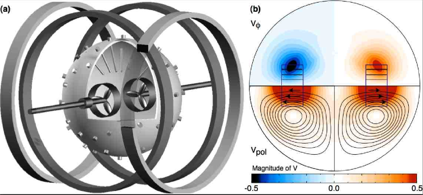
Figure 1: (a) A schematic of the Madison Dynamo Experiment. The sphere is $1\mbox{ m}$ in diameter and filled with $105$–$110\ ^{\circ}$C liquid sodium. High speed flows are created by two counter rotating impellers. Two sets of coils, one coaxial and one transverse to the drive shafts, are used to apply various magnetic fields for probing the experiment. (b) Contours of the toroidal velocity $v_{\phi}$ and contours of the poloidal flow stream function $\Phi$ where $\bm{\mathrm{v}}_{pol}=\nabla\Phi\times\nabla\phi$, of the axisymmetric double vortex flow generated by the impeller model. The region of forcing is shown schematically along the symmetry axis.

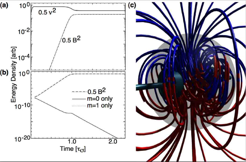
Figure 2: (a) The kinetic and magnetic energy densities shown versus time with $Rm=$159 and $Pm=1$. The time is in units of the resistive diffusion time $\tau_{\sigma}=\mu_{0}\sigma a^{2}$. (b) The contributions to the total magnetic energy density from the $m=1$ transverse dipole and the axisymmetric $m=0$ modes. (c) Magnetic field lines of a saturated dynamo state for a laminar flow with $Rm=150$.

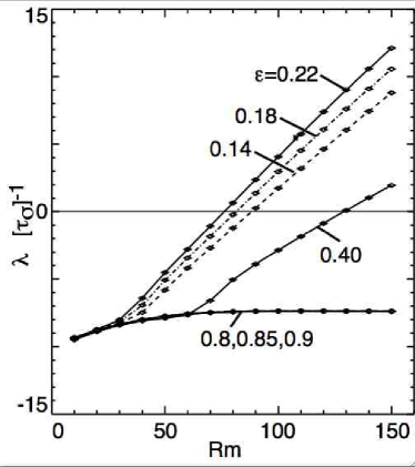
Figure 3: The dependance of the linear growth rate of the least-damped magnetic eigenmode on impeller pitch $\epsilon$. The transition from damped to growing ($\lambda=0$ point) defines the critical magnetic Reynolds number; $Rm<Rm_{crit}$ to a growing magnetic eigenmode.

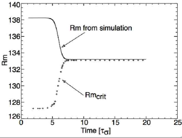
Figure 4: $Rm$ and $Rm_{crit}$ evolution during the saturation phase of a laminar dynamo. $Rm_{crit}$ is calculated from linear stability for each instantaneous velocity field during the simulation. In saturation, $Rm=Rm_{crit}$.

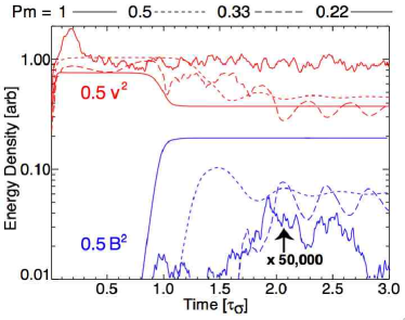
Figure 5: The magnetic and kinetic energy densities for runs with fixed $Rm$ ($Rm=165\pm 3\%$) but different $Pm$ versus time in $\tau_{\sigma}$. Note that $Pm=0.33$ shows a relaminarization of turbulent flow while $Pm=0.22$ is barely amplifying the initial noise and is shown multiplied by 50,000.

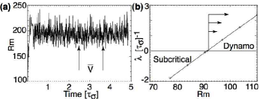
Figure 6: (a) Rm as a function of time. Taking a series of flows over the range shown the mean flow is calculated giving $Rm=193$ and $Re=863$. (b) The kinematic analysis of the average flow, where only Eq. 6 is evolved, and $Rm$ is varied, to determine $Rm_{crit}\ =\ 91.5$.

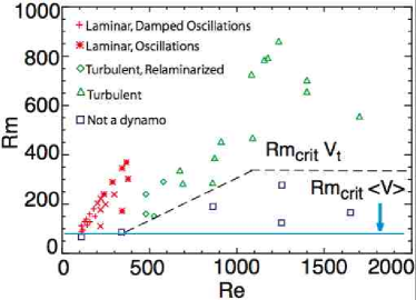
Figure 7: $Re-Rm$ phase diagram. A number of simulations whose hydrodynamic and final saturated states are documented in Fig. 5. $Rm_{crit}$ for the mean flow $\left<{\bf V}\right>$ is essentially independent of $Re$, while the effective dynamo threshold grows with $Re$. The dashed line shows the qualitative behavior of the dynamo threshold in turbulent flows ($V_{t}$).

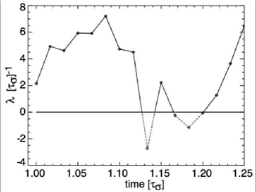
Figure 8: The growth rate of the dominant eigenmode calculated for a time-series of flow profiles.

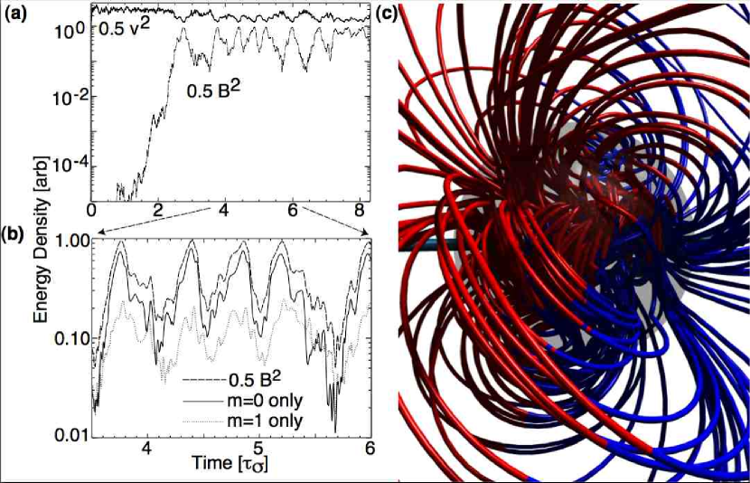
Figure 9: (a) The energy density of a turbulent dynamo with $Rm=337$ and $Re=674$. (b) The energy density of the axisymmetric magnetic field ($m=0$) and the nonaxisymmetric dynamo ($m=1$). (c) Magnetic field lines of the turbulent saturated dynamo

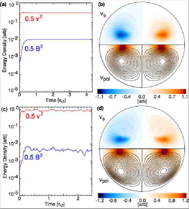
Figure 10: Simulations with an externally-applied, axisymmetric magnetic field. (a) Kinetic and magnetic energy densities for a Re=116 (laminar), Rm= 70 (subcritical) simulation. (b) the resulting flow. (c) Kinematic and magnetic energy densities for an Re=1803 (turbulent), Rm= 108 (subcritical) simulation. (d) The axisymmetric, time averaged velocity field for the turbulent simulation. The time average is over the time interval 0.3-2.4 $\tau_{\sigma}$, which is roughly $30$ decorrelation times.

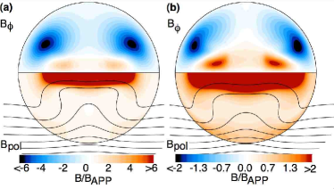
Figure 11: (a) The magnetic field for a laminar flow described in Fig. 10. The resulting total magnetic field (the sum of the externally applied field and those generated by the currents in the liquid metal) is shown as a multiple of the applied magnetic field. (b) The time-averaged magnetic fields, scaled to the applied field, for a turbulent flow [Rm=107 (subcritical), Re=1803]. The peak internal poloidal magnetic field is $9.3$ times larger than the applied field.

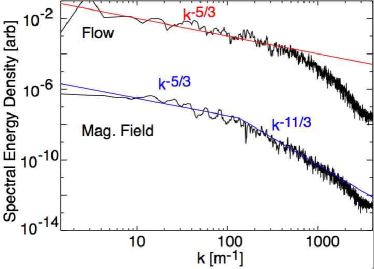
Figure 12: The wavenumber spectrum computed from frequency spectrum of fluctuations from $6\tau_{\sigma}$ of flow (fitted with the red $k^{-5/3}$ curve) output at a position ($r\sim 0.75\ a$, $\theta\sim\pi/2$, $\phi$=$0$) with a weak applied magnetic field of $B_{0}\sim 51.3$ G, fitted with the blue $k^{-5/3}$ at low $k$ and $k^{-11/3}$ at large $k$. For this simulation, $Rm=130$, and $Re=1450$ and fluctuations are assumed to be due to convection of spatial variations in the field. The dispersion relation is $\omega=k\left<V\right>$.

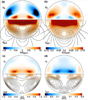
Figure 13: The magnetic field (a) generated by the mean-flow EMF $\left<\bm{\mathrm{V}}\right>\times\left<\bm{\mathrm{B}}\right>$. The peak internal poloidal magnetic field is $11.2$ times larger than the applied field. The magnetic field (b) generated by the turbulent EMF $\left<\widetilde{\bm{\mathrm{v}}}\times\widetilde{\bm{\mathrm{b}}}\right>$. (c) The currents associated with (a), and (d) the currents associated with (b). The turbulent flow has [$Rm=107$ (subcritical), $Re=1803$] and an externally generated magnetic field applied along the symmetry axis. The time average is taken over 2.1$\tau_{\sigma}$. Magnetic fields are scaled to the strength of the applied field.

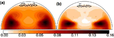
Figure 14: The turbulent and helical fluctuations for the simulation described in Fig. 12 (a) The average of the squared turbulent fluctuations as a multiple of the peak squared mean flow. (b) The time average of the kinetic helicity fluctuations $\left<\widetilde{\bm{\mathrm{v}}}\cdot\nabla\times\widetilde{\bm{\mathrm{v}}}\right>$ as a multiple of the volume-averaged helicity of the mean flow.

IV Turbulent Dynamos

To investigate the effect of turbulence on the dynamo transition, simulations are performed at lower $Pm$ (higher $Re$). The flow changes from laminar to turbulent at $Re\approx 420$. Above this value, a hydrodynamic instability grows exponentially on approximately an eddy-turnover time scale $\tau_{c}$ with a predominantly $m=1$ spatial structure. Through nonlinear coupling, the instability quickly leads to strongly-fluctuating turbulent flows (a detailed discussion of the spectrum of the turbulence is deffered to Sec. V). Fluctuations about the mean flow exist at all scales, including variations in the large-scale flow responsible for the dynamo. The turbulence is inhomogenous with boundary layers, localized forcing regions, and strong shear layers.

The effect of these fluctuations on the dynamo onset conditions and on the resulting saturation mechanism depends sensitively upon the viscosity (parameterized by $Pm$). Figure 5 shows an example of the broad range of dynamics exhibited by decreasing $Pm$, for an approximately fixed value of $Rm$. The magnetic field dynamics fall into several regimes depending on $Re$: the laminar dynamo, a dynamo that starts turbulent, but relaminarizes the saturated flow, a turbulent dynamo, and finally a turbulent flow with no dynamo. At $Pm=1$, the viscosity is large enough to keep both the magnetic field and velocity field fully laminar. The spectrum is dominated by the driven velocity field and by the magnetic eigenmode, and the saturation mechanism is the Lorentz braking and modification to the flow mentioned above.

For $Pm=0.33$, Fig. 5 shows a flow that is initially turbulent, but the saturated state is laminar. The turbulent saturation of the magnetic field results in a reduction in the fluctuations of the flow since the Lorentz braking has reduced $Re$ below the hydrodynamic instability threshold (decreasing $Re$ from 496 to 320). A hydrodynamic case, which evolves the flow with $\bm{\mathrm{B}}=0$, shows that flow turbulence persists without the addition of a magnetic field into the system. The $Re$ threshold distinguishing the turbulent saturated state from a relaminarized saturation is $Re\sim 630$.

If $Rm$ is fixed near the experimental maxima while $Re$ is increased beyond $700$, no dynamo is observed. Despite the fact that the mean flow still satisfies the requirements of a kinematic dynamo, the turbulent flow does not produce a growing magnetic field. Evidently, it is the turbulent fluctuations about the mean flow that prevent field growth. Using the mean flow (averaged over several resistive times) for the $Pm=0.22$ (with $Rm$=190, $Re$=863) as a prescribed flow in a kinematic evolution of the induction equation gives $Rm_{crit}\approx 93$, as shown in Fig. 6. Even though the average flow has $Rm$ well above $Rm_{crit}$ there is no dynamo. However, when the conductivity is doubled such that $Rm=388$ a turbulent dynamo reemerges in the simulation. Hence, an empirical critical magnetic Reynolds number, $Rm_{crit,T}$ can be defined which depends on $Re$ through the degree of turbulent fluctuations in the flow.

These results are consistent with the dynamo transition being affected by the turbulent resistivity of Eq. 3. From analysis of the simulation results, the correlation time $\tau_{c}$, the eddy scale size $\ell_{v}$, i and fluctuation levels $C=\tilde{v}/V_{0}$ have been determined in order to estimate the parameters in $\sigma_{T}$ under the assumption that the homogeneous turbulence results roughly apply to this bounded, inhomogeneous flow. Typical volume averaged values measured in the $Rm=190,\ Re=863$ simulation are: $\ell_{v}=0.022a$, $C=0.45$, and $\tau_{corr}=0.041\tau_{\sigma}$, which yields a volume-averaged conductivity reduction of $\sigma_{T}/\sigma=0.461$. The diminished conductivity yields $Rm_{crit,T}=238$. The results from all of the simulations are summarized in Fig. 7 which shows that an increasing $Rm$, at fixed $Re$ reestablishes field growth where turbulent fluctuations had previously suppressed the dynamo. The dashed line in Fig. 7 shows that the correlation length and constant $C$ increase with $Re$ and eventually asymptote when the conductivity is effectively reduced by $70$ %.

The simulated turbulence has no de facto scale separation. This might appear to pose a problem, given that our interpretation of the effect of turbulence is the introduction of a turbulent resistivity, and the turbulent resistivity of Mean Field Theory (MFT) krause80 is usually couched in scale separation arguments. However, it should be noted that the scale separation requirement associated with the $\alpha$ and $\beta$ effects of MFT does not enter into the form of $\beta$, but does guarantee that $\alpha<\beta$. This is because $\alpha$ is proportional to helicity whereas $\beta$ is proportional to energy while $\alpha$ multiplies a lower derivative of the mean field than does $\beta$. In this sense the lack of scale separation in the simulations is consistent with the apparent weakness of a turbulent-$\alpha$ effect in a regime with a turbulent resistivity.

While the simulations are limited to $Re<2000$ by computational speed and storage, we believe the simulations capture the dominant effect since the fluctuations at the largest scales are the strongest contributers to the turbulent resistivity by the following argument. In Kolmogorov turbulence k41 the spectrum is $E(k)\propto\epsilon^{2/3}k^{-5/3}$, where $\epsilon$ is the energy dissipation rate. Thus the turbulent resistivity goes as $[\int_{k_{0}}^{k_{\nu}}q^{-2}E(q)dq]^{-1/2}\sim\epsilon^{1/3}k_{0}^{-4/3}$, where $k_{0}$ is the wavenumber of the large scale eddies and $k_{\nu}$ is the dissipation scale wavenumber. In K41 turbulence, $k_{\nu}\propto Re^{3/4}$, as $Re$ becomes large in comparison to $Rm$, the effect of turbulent fluctuations on conductivity will asymptote to a fixed value. It should be noted that the simple dimensional analysis used for estimating the turbulent resistivity reflects isotropic homogenous turbulence and is derived in the limit that there is no mean flow; this dynamo relies almost entirely on the presence of a mean flow.

An alternative viewpoint, consistent with the phenomenological interpretation of enhanced resistivity put forward here, is that the large-scale variations in the velocity field are continuously changing the spatial structure and growth rates of the magnetic eigenmodes of the system. A more thorough treatment of the dynamic variation of dominant eigenmodes can be found for a slightly different problem in terry06 . Two effects can be important. First, the instantaneous growth rate of the least damped eigenmode fluctuates between growing and damped. For a run with $Rm=193$, $Re=893$ and $\epsilon=0.4$, shown in Fig. 8, a dynamo occurs only when the flow spends sufficient time in phases which are kinematic dynamos. The kinematic growth rate is most often positive, consistent with the time averaged flow having growing magnetic field solutions, yet the modifications made to the flow during the subcritical periods are sufficient to stop the dynamo. Second, the turbulence couples energy from the growing magnetic eigenmode into spatially-similar damped eigenmodes. As the flows evolve, the spatial structure of the eigenmodes change. The magnetic field structure of a single eigenmode at some previous instant in time must be described in terms of several modes after the flow changes. This transfer of energy from the primary mode is equivalent to enhanced dissipation. Analysis of the eigenmode structure shows that the least damped eigenmode during a nondynamo phase in Fig. 8 varies between the marginally stable nonaxisymmetric dipole and a stable axisymmetric magnetic mode. Thus the flow imparts energy to a spatially similar, but distinct magnetic eigenmode.

Finally, it should be noted that distinguishing between growing and damped magnetic fields is difficult in the turbulent simulations. Typically, the turbulent runs have been limited to durations of less than 10 $\tau_{\sigma}$. The transition may also be considerably more complex as seen in Fig. 5 where magnetic energy of the $Pm=0.22$ simulation may show intermittent growth near $Rm_{crit,T}$. The simulations are thus consistent with intermittent excitation of the dynamo eigenmode by the mean flow. The peak magnetic energy is limited by the magnitude of the initialized noise the simulation is started with instead of the backreaction with the flow. This effect is especially relevant when the magnetic field is sustained by an external source as shown in Section V.

A dynamo still occurs in these flows for sufficiently large $Rm$ (keeping $Re$ fixed, growing magnetic energy is detected for sufficiently large $Pm$). An example of a time evolution and spatial structure of a saturated turbulent magnetic field is shown in Fig. 9 for a simulation with $Rm=337$ and $Re=674$. An $m=1$ transverse dipole field is still present, as in the case of the laminar dynamo in Fig. 2, however this turbulent dynamo is now dominated by the presence of a large $m=0$ field, aligned with the axis of symmetry of the impellors as shown in Fig. 9(b). This component, by itself, would appear to violate Cowling’s theorum cowling33 , and so it must result from non-axisymmetric components of the velocity field and the magnetic field. Thus it appears probable that the nature of dynamo has changed fundamentally from a simple eigenmode driven by the two vortex flow, to a dynamo in which the turbulent fluctuations may be responsible for generating the large-scale magnetic field.

V Simulations of a subcritical turbulent flow with a weak, externally-applied magnetic field

As a means of further highlighting the different physics and conditions underlying turbulent and laminar dynamos, subcritical flows are simulated with focus on the potential role of fluctuation driven currents in the self-excitation process. Subcritical flows have $Rm<Rm_{crit}$, and are not expected to lead to self-excited magnetic fields. The MHD behavior is investigated by applying a magnetic field which is generated by currents flowing in coils external to the sphere. The configuration studied is similar to the set of experiments described in Ref. spence06 , and is deliberately set up as an axisymmetric system in which fluctuation driven currents can be easily detected.

The numerical technique employed is similar to the dynamo simulations described above in all but one respect, namely a different boundary condition is used with $C_{\ell,m}\neq 0$ in Eq. 25. These boundary conditions match the magnetic field to a scalar magnetic potential $\bm{\mathrm{B}}=-\nabla\Phi_{m}$, which is valid in the region between the surface of the sphere and the external magnets. $\Phi$ satisfies Laplace’s equation and its solution is well known:

$$\Phi_{m}(r,\theta,\phi)=\sum_{\ell,m}\left(A_{\ell,m}r^{\ell}+D_{\ell,m}r^{-(\ell+1)}\right)Y_{\ell}^{m}(\theta,\phi),$$ (29)

where $Y_{\ell}^{m}(\theta,\phi)$’s are the spherical harmonics. The $D_{\ell,m}$ terms represent the magnetic field generated by currents in the sphere, and the coefficients $A_{\ell,m}$ can be chosen to describe a magnetic field of arbitrary shape and orientation applied by currents external to the sphere. In this paper and in the simulations described below, a uniform magnetic field is applied along the symmetry axis of the forcing terms, and is characterized by a single coefficient $A_{1,0}$, all higher order terms being zero. The applied magnetic field, $B_{1,0}$, is weak enough so that it does not alter the large-scale flow. The strength of the applied magnetic field is moderated by keeping the Stuart number $N\equiv\sigma aB_{1,0}^{2}/\rho\bm{\mathrm{v}}_{0}<0.1$. In sodium, with a $Rm\sim 100$, $N\sim 0.1$ would correspond to an applied field of $156$ gauss. The applied field for these simulations is uniform and applied along the impeller axis with $B_{1,0}\sim 57$ gauss and $N\sim 10^{-2}$. However, since the velocity fluctuations decrease with scale, the Stuart number increases with scale, indicating the Lorentz force may influence small-scale fluid motion. Examples of such simulations are shown in Fig. 10, where the kinetic energy and magnetic energy are shown for laminar and turbulent runs.

For the laminar flow, the induced currents and resulting magnetic field are purely due to the magnetic field interacting with the mean flow, as seen in Fig. 11(a). Two main effects are observed. First, induced toroidal currents compress lines of poloidal magnetic field near the axis of the device. The lines are pulled outward at the poles and inward at the equator. The net result is a reduction of the poloidal field strength at the equator in the outer region, and a large amplification at the axis (the peak poloidal field is $18$ times the applied field). Second, poloidal currents generate a toroidal magnetic field. These currents are generated by the well-known omega effect of dynamo theory whereby differential toroidal rotation of the fluid is able to stretch the field into the toroidal direction moffatt78 . The amplitude of the peak toroidal field is greater than $6$ times the applied field.

The transition to turbulence is still characterized by the same $Re\sim 420$ threshold described above, since the Stuart number for the applied magnetic field is small. Below this threshold, the nonaxisymmetric part of the flows is negligible while above this threshold nonaxisymmetric fluctuations in both $\bm{\mathrm{B}}$ and $\bm{\mathrm{V}}$ can be as large as $40\%$ of the mean values. The geometry of the simulations (axisymmetric drive terms aligned with the applied magnetic field) makes it possible to separate mean, axisymmetric quantities and fluctuating quantities,

$$\bm{\mathrm{B}}=\left<\bm{\mathrm{B}}\right>+\widetilde{\bm{\mathrm{b}}}\mbox{ and }\bm{\mathrm{v}}=\left<\bm{\mathrm{V}}\right>+\widetilde{\bm{\mathrm{v}}},$$ (30)

where the brackets denote a time average over several resistive times. In practice, $\left<\bm{\mathrm{B}}\right>$ and $\left<\bm{\mathrm{V}}\right>$ are axisymmetric for sufficiently long time averages. Using these definitions, the time-averaged magnetic fields can be computed for laminar and turbulent flows, shown in Fig. 11.

Both laminar and turbulent flows demonstrate toroidal field production and expulsion of poloidal flux. Laminar and turbulent results differ in several important ways, however, which are attributable to the currents being driven by MHD fluctuations. First, the toroidal field is greatly reduced in the turbulent run. The induced toroidal field is $6$ times the applied field strength in the laminar flow and is only twice the applied field in the turbulent case. Second, the peak poloidal field is halved in the turbulent run, as shown in Fig. 11(a). Third, there is a net magnetic dipole moment associated with the induced field which is not present in the laminar case. These differences are partially the result of a difference between the mean flows in the two cases, but are mostly a due to a strong influence of the turbulence on the current generation. This can be interpreted in the context of a modification to the mean-field Ohm’s law, i.e. turbulence-generated currents are modifying the large-scale, mean magnetic field.

A turbulent EMF is possible because of the flow fluctuations and the magnetic field generated by the passive advection of the applied magnetic field by the Kolmogorov-like turbulence in the velocity field. Fig. 12 shows the wavenumber spectrum as estimated from the frequency spectrum of the fluctuations in both $V$ and $B$ at a fixed point in the simulation using the Taylor hypothesis to map frequency fluctuations to wavenumber $\omega\sim k\left<V\right>$. It is clear that both the velocity field and magnetic field have an inertial range ($k^{-5/3}$) and a dissipation scale, although the dissipation scales are at different values of $k$. The $k^{-5/3}$ scaling of the velocity field (the inertial range) is expected from the Kolmogorov theory of hydrodynamic turbulence. The dissipation scale for the fluid turbulence is expected to be at $k_{\nu}\sim Re^{-3/4}=235$ which is roughly the position of the viscous cutoff shown in Fig. 12. The limited inertial range at low k, is primarily due to constraints on long-time averages of the data imposed by computational speed.

The $k^{-5/3}$ scaling of the magnetic field corresponds to the weak-field approximation in which the induced magnetic fluctuations are due to advection of the mean magnetic field by the mean flow nornberg06 for $k<k_{\sigma}\sim Rm/a$. The $k^{-11/3}$ power law results from a balance between the mean magnetic field advected by turbulence and the resistive dissipation of magnetic fluctuations. The dissipation scales are evident from the knee in the wave number spectra of Fig. 12. The spectrum is constructed from the power spectrum of the value of $B_{r}$ near the equator. Consequently, the magnetic field gains structure at smaller scales as $Rm$ increases, down to scale sizes of $\ell_{\sigma}=2\pi/k_{\sigma}=4.8$ cm at $Rm=130$.

The simultaneous fluctuating magnetic and velocity fields can potentially drive current in a mean-field sense. The motional EMF can be written as

$$\bm{\mathrm{v}}\times\bm{\mathrm{B}}=\left<\bm{\mathrm{V}}\right>\times\left<\bm{\mathrm{B}}\right>+\left<\bm{\mathrm{V}}\right>\times\widetilde{\bm{\mathrm{b}}}+\widetilde{\bm{\mathrm{v}}}\times\left<\bm{\mathrm{B}}\right>+\widetilde{\bm{\mathrm{v}}}\times\widetilde{\bm{\mathrm{b}}},$$ (31)

where the mean-fields have been separated from the fluctuating parts. The time averages must be taken over times long compared to a turbulent decorrelation time and comparable to the resistive diffusion time. Since the turbulent decorrelation time, $\tau_{C}\sim 0.05\tau_{\sigma}$, integrating the induction term over several resistive times yields

$$\left<\bm{\mathrm{v}}\times\bm{\mathrm{B}}\right>=\left<\bm{\mathrm{V}}\right>\times\left<\bm{\mathrm{B}}\right>+\left<\widetilde{\bm{\mathrm{v}}}\times\widetilde{\bm{\mathrm{b}}}\right>.$$ (32)

An important question is whether the currents generated in the simulation are primarily due to the motional EMF associated with the mean-flow and the mean magnetic field, $\left<\bm{\mathrm{V}}\right>\times\left<\bm{\mathrm{B}}\right>$, or if there are also currents driven by the turbulent EMF $\left<\widetilde{\bm{\mathrm{v}}}\times\widetilde{\bm{\mathrm{b}}}\right>$. This can be investigated by examining the various terms in Ohm’s Law

$$\bm{\mathrm{E}}=\eta\bm{\mathrm{J}}-\left<\bm{\mathrm{V}}\right>\times\left<\bm{\mathrm{B}}\right>+\left<\widetilde{\bm{\mathrm{v}}}\times\widetilde{\bm{\mathrm{b}}}\right>$$ (33)

It is clear that in steady-state there can be no inductive electric field in the toroidal direction since the poloidal flux is constant. Axisymmetry precludes an electrostatic potential from driving current in the toroidal direction, and so the toroidal current can only be generated by the mean-flow and the turbulent EMF. Thus any currents driven in the toroidal direction contribute to the poloidal magnetic field. Fig. 13(c) shows the currents driven by these fluctuations and their corresponding magnetic field (a). The fluctuation-induced magnetic field is $3.5$ times larger than the applied field and comprises a third of the total field strength.

It has been recently shown that an axisymmetric flow and axial magnetic field cannot induce a dipole moment in any simply-connected bounded system spence06 . This is essentially due to the fact that the flow outside the conducting region is zero, while the streamlines of flow perpendicular to the magnetic flux are closed and bounded within the conducting region. Only a turbulent EMF can create the dipole moment. With a weak applied field in a turbulent fluid, averaging over several eddy turnover times and averaging along $\hat{\bm{\phi}}$ eliminates the nonaxisymmetric component of the current, therefore the only nontrivial component of the dipole moment is

$$\mu_{Z}=\oint d^{3}xr\sin{\theta}J_{\phi}.$$ (34)

The toroidal current generated by $\left<\widetilde{\bm{\mathrm{v}}}\times\widetilde{\bm{\mathrm{b}}}\right>$ from Eq. 32, is shown in Fig. 13(d) and the associated dipole moment (antiparallel to the external field) is clearly seen in Fig. 13(b). Alternatively, the EMF due to $\bm{\mathrm{V}}$ and $\bm{\mathrm{B}}$ gives rise to a hexapole magnetic field (in Fig. 13(a)). The resulting poloidal field reduces the surface magnetic field by $20\%$. The largest values of the turbulent toroidal current occur where the omega effect is also large.

The EMF which generates the toroidal current associated with the induced dipole moment may very well resemble the currents driven by the well-known $\alpha$-effect. The omega effect generates a toroidal magnetic field which would in turn would support a current of the form $J_{\phi}=\alpha B_{\phi}$. It is impossible to uniquely identify the current this way, however. A non-uniform $\beta$-effect (change in local resistivity) could equally well explain the results. To do this would require separating the currents associated with the helical fluctuations from the non-helical fluctuations and this has not yet been done. A local analysis of the turbulent helicity content in Fig. 14(b) shows that helical fluctuations exist that might be expected to drive a current through the $\alpha$-effect.

To study Ohm’s law in the poloidal direction requires a full treatment of the poloidal electric field since an electrostatic potential is not ruled out by symmetry arguments. In MHD, the electrostatic potential is assumed to instantaneously adjust itself to ensure that $\bm{\nabla}\cdot\bm{\mathrm{J}}=0$. This can only be assured if the divergence of the motional EMFs is balanced by a spatially varying electric field

$$\boldsymbol{\nabla}\cdot{\bf\bm{\mathrm{E}}}=-\nabla^{2}\Phi-\nabla^{2}\tilde{\Phi}=\boldsymbol{\nabla}\cdot{\bf\bigl{(}\left<\bm{\mathrm{V}}\right>\times\left<\bm{\mathrm{B}}\right>+\left<\widetilde{\bm{\mathrm{v}}}\times\widetilde{\bm{\mathrm{b}}}\right>\bigr{)}},$$ (35)

where $\Phi$ and $\tilde{\Phi}$ are electrostatic potentials due to the stationary EMF, and turbulent EMF respectively. Thus, a poloidal current can be associated with the mean-flows and the turbulent EMF respectively:

$$\bm{\mathrm{J}}_{pol} = \sigma\left(-\nabla\Phi+\left<\bm{\mathrm{V}}\right>\times\left<\bm{\mathrm{B}}\right>_{pol}\right)$$ (36)

$$\tilde{\bm{\mathrm{J}}}_{pol} = \sigma\left(-\nabla\tilde{\Phi}+\left<\widetilde{\bm{\mathrm{v}}}\times\widetilde{\bm{\mathrm{b}}}\right>\right).$$ (37)

When analyzing Ohm’s law in the poloidal direction, it is necessary to first compute these potentials, which has been done for the poloidal currents in Fig. 13.

The simulations indicate there is a strong poloidal current, shown in Fig. 13(d), associated with the fluctuations. The current acts to greatly reduce the toroidal magnetic field generated by a comparable laminar flow, thereby reducing the toroidal field in the core. This resembles the diamagnetic $\gamma$-effect krause80 , due to gradients in the turbulence intensity. The $\alpha$-effect is the diagonal part of a mean-field tensor: $\bm{\mathrm{J}}=\sigma\bm{\alpha}\cdot\bm{\mathrm{B}}$. The off-diagonal terms can also be written so that $\bm{\mathrm{J}}=\sigma\bm{\gamma}\times\bm{\mathrm{B}}$. Figure 14(a) shows the squared velocity fluctuations decrease away from the axis of symmetry with the polar radius, $\rho$. For isotropic turbulence, the inhomogeneity in the fluctuations would give rise to a $\gamma$-effect of the form $-\sigma\bm{\gamma}(\rho)\times\bm{\mathrm{B_{\mathrm{T}}}}$ with $\bm{\gamma}\propto\bm{\nabla}\mathrm{v}^{2}$. The poloidal current due to turbulent diamagnetism would counteract the toroidal magnetic field caused by the omega effect. Comparison between Fig.13(a) with Fig.14(b) shows that regions of steep gradients in the turbulent fluctuations correspond to regions of strong fluctuation induced poloidal current.

VI Summary

The role of turbulence in generating current and moderating the growth of magnetic fields has been studied for the Madison Dynamo experiment using 3D numerical simulations. A simple forcing term has been used to model impellors in the experiment; at sufficient forcing the flow becomes turbulent. Two regimes were explored: one with an external applied magnetic field and flow subcritical to the dynamo instability and one with no external field and super-critical flow. The role of the turbulence on current generation and self-excitation is marked.

The onset conditions for the dynamo instability are governed not only by $Rm$ but also by the magnetic Prandtl number $Pm$. At $Pm\sim 1$, the transition and saturation agree with laminar predictions and are considered laminar dynamos. At lower $Pm$, $Rm_{crit}$ increases, consistent with a reduction in conductivity due to turbulent fluctuations. However, at higher $Rm$ the character of the dynamo changes; its symmetry suggests that turbulence driven currents are important in the self-excitation process. The $Pm$ values in the simulations are still orders of magnitude larger than in liquid-metal experiments (and for geo and solar dynamos) due to memory and speed limitations of computers, and so experiment support is critical for verifying these results.

To quantify currents driven by fluctuations in the experiment, simulations of subcritical flows have been performed, and the currents driven by the turbulent fluctuations have been observed directly. The main effect of the turbulence on an externally-applied magnetic field is the reduction of field strength compared with those computed for laminar flows. The laminar two-vortex flow compresses the applied poloidal magnetic flux near the axis of symmetry and through toroidal flow shear creates a strong toroidal magnetic field. Both effects are reduced in turbulent flows. The mean flow produced at large Reynolds numbers differs from its laminar counterpart, which accounts for some of the discrepancy between the build-up of toroidal field and flux compression of the poloidal field observed in the laminar and turbulent fluids. However, it has also been shown that a fluctuation driven EMF drives current which modifies the large-scale magnetic field, both generating a dipole moment and expelling toroidal flux from the interior region.

We would like to thank C. Sovinec, S. Prager, J. Wright, and E. Zweibel for many useful discussions. This work was supported by the National Science Foundation.

References

- (1) H. Moffatt, Magnetic field generation in electrically conducting fluids (Cambridge University Press, Cambridge, 1978).
- (2) S. Childress and A. Gilbert, Stretch, Twist, Fold: The fast dynamo (Springer, Berlin, 1995).
- (3) R. Kraichnan and S. Nagarajan, Phys. Fluid 10, 859 (1967).
- (4) U. Frisch, A. Pouquet, J. Léorat, and A. Mazure, J. Fluid Mech. 68, 769 (1975).
- (5) A. Pouquet and G. Patterson, J. Fluid Mech. 85, 305 (1978).
- (6) A. Alexakis, P. Mininni, and A. Pouquet, On the inverse cascade of magnetic helicity, http://arxiv.org/abs/physics/0509069, 2005.
- (7) E. Bullard and H. Gellman, Phil. Trans. R. Soc. Lond. A 247, 213 (1954).
- (8) P. H. Roberts, Phil. Trans. Roy. Soc. London A 272, 60 (1972).
- (9) D. Gubbins, Phil. Trans. R. Soc. Lond. A 274, 493 (1973).
- (10) G. Glatzmaier, J. Comp. Phys. 55, 481 (1984).
- (11) G. Glatzmaier and P. Roberts, Phys. Earth Plan. Int. 91, 63 (1995).
- (12) G. Glatzmaier, Ann. Rev. Earth Planet. Sci. in press (2002).
- (13) A. Kageyama and T. Sato, Phys. Plasmas 2, 1421 (1995).
- (14) A. Kageyama and T. Sato, Phys. Plasmas 4, 1569 (1997).
- (15) W. Kuang and J. Bloxham, Nature 389, 371 (1997).
- (16) M. Meneguzzi, U. Frisch, and A. Pouquet, Phys. Rev. Lett. 47, 1060 (1981).
- (17) F. Cattaneo and D. Hughes, Phys. Rev. E 54, 4532 (1996).
- (18) W. Müller, D. Biskamp, and R. Grappin, Phys. Rev. E 67, 066302 (2003).
- (19) S. Boldyrev and F. Cattaneo, Phys. Rev. Lett. 92, 144501 (2004).
- (20) A. Schekochihin, S. Cowley, J. Maron, and J. McWilliams, Phys. Rev. Lett. 92, 054502 (2004).
- (21) Y. Ponty, P. Mininni, D. Montgomery, J. Pinton, H. Politano, and A. Pouquet, Phys. Rev. Lett. 94, 164502 (2005).
- (22) A. Gailitis, A. Lielausis, E. Platacis, S. Dement’ev, A. Cifersons, G. Gerbeth, T. Gundrum, F. Stefani, M. Christen, H. Hänel, and G. Will, Phys. Rev. Lett. 84, 4365 (2000).
- (23) A. Gailitis, A. Lielausis, E. Platacis, S. Dement’ev, A. Cifersons, G. Gerbeth, T. Gundrum, F. Stefani, M. Christen, and G. Will, Phys. Rev. Lett. 86, 3024 (2001).
- (24) A. Gailitis, A. Lielausis, E. Platacis, G. Gerbeth, and F. Stefani, Phys. Plasmas 71, 2838 (2004).
- (25) R. Stieglitz and U. Müller, Phys. Fluids 13, 561 (2001).
- (26) U. Müller and R. Stieglitz, Phys. Fluids 16, (2004).
- (27) U. Müller and R. Stieglitz, J. Fluid Mech. 498, 31 (2004).
- (28) A. Reighard and M. Brown, Phys. Rev. Lett. 86, 2794 (2001).
- (29) U. Müller and R. Stieglitz, Nonlinear Processes in Geophysics 9, 165 (2002).
- (30) P. Roberts and G. Glatzmaier, Rev. Mod. Phys. 72, 1081 (2000).
- (31) F. Cattaneo, in Modeling of Stellar Atmospheres, ASP Conference Series, edited by N. Piskunov, W. Weiss, and D. Gray (IAU Publications, Paris, 2002).
- (32) F. Pétrélis, M. Bourgoin, L. Marié, J. Burguete, A. Chiffaudel, F. Daviaud, S. Fauve, P. Odier, and J.-F. Pinton, Phys. Rev. Lett. 90, 174501 (2003).
- (33) N. Peffley, A. Cawthorne, and D. Lathrop, Phys. Rev. E 61, 5287 (2000).
- (34) R. O’Connell, R. Kendrick, M. Nornberg, E. Spence, A. Bayliss, and C. Forest, in Proceedings of the NATO Advanced Research Workshop on Dynamo and Dynamics, a Mathematical Challenge, Cargése, France, Vol. 26 of Nato Science Series, edited by P. Chossat, D. Armbustier, and I. Oprea (Kluwer, Dordrecht, 2001), p. 59.
- (35) L. Quartapelle and M. Verri, Computer Physics Communications 90, 1 (1995).
- (36) C. Canuto, M. Hussaini, A. Quarteroni, and T. Zang, Spectral Methods in Fluid Dynamics (Springer-Verlag, Berlin, 1988), p. 84.
- (37) M. Dudley and R. James, Proc. R. Soc. Lond. A 425, 407 (1989).
- (38) R. Holme and J. Bloxham, J. Geophys. Res. 101, 2177 (1996).
- (39) M. Nornberg, E. Spence, R. Kendrick, C. Jacobson, and C. Forest, Phys. Plasmas 13, 055901 (2006).
- (40) A. N. Kolmogorov, Dokl. Akad. Nauk. 30, 299-303 (1941).
- (41) P. Terry, D. Baver, and S. Gupta, Phys. Plasmas 13, 022307 (2006).
- (42) T. Cowling, Mon. Not. R. Astr. Soc. 94, 39 (1933).
- (43) E. Spence, M. Nornberg, C. Jacobson, R. Kendrick, and C. Forest, Phys. Rev. Lett. 96 055002 (2006).
- (44) K. Krause and K. Rädler, Mean–field Magnetohydrodynamics and Dynamo Theory (Pergamon Press, Oxford, 1980).