On the $1/f$ Frequency Noise in Ultra-Stable Quartz Oscillators

Abstract

The frequency flicker of an oscillator, which appears as a $1/f^{3}$ line in the phase noise spectral density, and as a floor on the Allan variance plot, originates from two basic phenomena, namely: (1) the $1/f$ phase noise turned into $1/f$ frequency noise via the Leeson effect, and (2) the $1/f$ fluctuation of the resonator natural frequency. The discussion on which is the dominant effect, thus on how to improve the stability of the oscillator, has been going on for years without giving a clear answer. This article tackles the question by analyzing the phase noise spectrum of several commercial oscillators and laboratory prototypes, and demonstrates that the fluctuation of the resonator natural frequency is the dominant effect. The investigation method starts from reverse engineering the oscillator phase noise in order to show that if the Leeson effect was dominant, the resonator merit factor $Q$ would be too low as compared to the available technology.

Symbol list
$A$	amplifier (voltage) gain
$b_{i}$	coefficient of the power-law representation of $S_{\mathchar 295\relax}(f)$
$b(t)$	resonator impulse response in the phase space
$B(s)$	Laplace transform of $b(t)$
$f$	Fourier frequency (near dc)
$f_{c}$	amplifier corner frequency, divides white and $1/f$ regions
$f_{L}$	Leeson frequency
$F$	amplifier noise figure
$h_{i}$	coefficient of the power-law representation of $S_{y}(f)$
$H(s)$	loop transfer function (Laplace transform)
$\mathcal{H}(s)$	loop transfer function (Laplace transf.) in the phase space
$j$	imaginary unit, $j^{2}=-1$
$k$	$1.38{\times}10{-23}$ J/K, Boltzmann constant
$P$, $P_{0}$	carrier power. Also $P_{a}$, $P_{b}$, $P_{m}$, etc.
$Q$	resonator merit factor
$R$	frequency-srability ratio
$s$	complex frequency, $s=\sigma+j\omega$, in Laplace transforms
$S(f)$, $S_{x}(f)$	single-sided power spectrum density (of the quantity $x$)
$t$	time
$T$, $T_{0}$	absolute temperature, reference temperature ($T_{0}=290$ K)
$v(t)$	(voltage) signal, as a funtion of time
$V_{0}$, $V_{i}$	peak carrier voltage
$y$	fractional frequency fluctuation, $y=\smash{\frac{\nu-\nu_{0}}{\nu_{0}}}$
$\alpha(t)$	fractional amplitude fluctuation
$\beta(s)$	resonator impulse response (Laplace transform)
$\nu$, $\nu_{0}$	frequency, carrier frequency
$\sigma_{y}(\tau_{m})$	Allan deviation of the quantity $y$
$\tau_{m}$	as in $\sigma_{y}(\tau_{m})$, measurement time
$\tau$	resonator relaxation time
$\mathchar 295\relax(t)$	oscillator phase fluctuation
$\Phi(s)$	Laplace transform of $\mathchar 295\relax(t)$
$\psi(t)$	amplifier phase fluctuation
$\Psi(s)$	Laplace transform of $\psi(t)$
$\omega$	angular frequency
Note: $\bm{\omega}$ is used as a shorthand for $\bm{2\pi\nu}$ or $\bm{2\pi f}$, and viceversa

1 Introduction and summary

In the domain of ultra-stable quartz oscillators used in the most demanding applications, like space and atomic fountain clocks, we notice that the frequency flicker is often the most critical parameter. The required stability is sometimes in the upper $10^{-14}$ (Allan deviation) at 1–30 s or so, which can only be achieved in the lower HF band (5–10 MHz), and after selection. In such cases, identifying the dominant flicker mechanism is far from being trivial. Whereas some authors strongly suggest that the amplifier noise can be the parameter that limit the frequency stability, rather than the flickering of the resonator natural frequency [walls95eftf, besson99eftf], the general literature seems not to give a clear answer. This conclusion results from a set of selected articles, which includes the measurement of the frequency stability [walls75im, rubiola00uffc] and the interpretation of the flicker noise of crystal resonators [kroupa88uffc, kroupa05pla]; the design fundamentals of the nowadays BVA resonators [besson77fcs]; some pioneering works on the low-frequency noise in quartz oscillators [brendel75im, driscoll75im]; more recent articles focusing on specific design solutions for ultra-stable oscillators [norton91fcs, norton95fcs, candelier98eftf, candelier03fcs, tuladhar97eftf]; and, as a complement, a thorough review of the SiO₂ crystal for the resonator fabrication is found in [brice85rmp]. Conversely, in everyday-life oscillators, which span from the low-cost XOs to the OCXOs used in telecommunications and instrumentation, the relative simplicity of the low-noise electronics required indicates that the frequency flicker is chiefly the $1/f$ fluctuation of the resonator.

In a previous work [rubiola05arxiv-leeson], now extended to more commercial products and laboratory prototypes, we have analyzed the phase noise spectrum of some oscillators, aiming at understanding the internal mechanisms and parameters. We look at the phase-noise spectrum from the right hand to the left, hence from the higher Fourier frequencies to the lower, matching theory, technology and physical insight. In this way we get information on the sustaining amplifier on the output buffer, on the Leeson effect and on the resonator.

In this article we first explain the phase noise mechanisms in amplifiers. Then we introduce the Leeson effect, which consists of the phase-to-frequency conversion of noise below the resonator cutoff (Leeson) frequency $f_{L}=\smash{\frac{\nu_{0}}{2Q}}$. Finally, we analyze the phase noise spectral density $S_{\mathchar 295\relax}(f)$ of a few oscillators. The conclusion that the resonator natural frequency is the main cause of frequency flickering is based on experimental facts. After taking away the effect of the output buffer, we calculate the frequency $f^{\prime\prime}_{L}$ at which the oscillator $f^{-3}$ line crosses the $f^{-1}$ line of the sustaining amplifier. Provisionally assuming that $f^{\prime\prime}_{L}$ is the the Leeson frequency, we observe that the resonator merit factor $Q_{s}=\smash{\frac{\nu_{0}}{2f^{\prime\prime}_{L}}}$ thereby calculated is far too low for a high-tech resonator. Conversely, under any reasonable assumption about the true merit factor, the Leeson effect is found at a frequency $f_{L}\ll f^{\prime\prime}_{L}$. Therefore the Leeson $f^{-3}$ line on the $S_{\mathchar 295\relax}(f)$ plot is well hidden below the resonator fluctuation.

2 Phase noise fundamentals

Let the quasi-perfect oscillator sinusoidal signal of frequency $\nu_{0}$

$$v(t)=V_{0}[1+\alpha(t)]\cos[2\pi\nu_{0}t+\mathchar 295\relax(t)]\leavevmode\nobreak\ .$$ (1)

where $\alpha(t)$ is the fractional amplitude noise, and $\mathchar 295\relax(t)$ is the phase noise. The AM noise is not essential to this work. The phase noise is best described in terms of $S_{\mathchar 295\relax}(f)$, i.e., the one-sided power spectral density of $\mathchar 295\relax(t)$, as a function of the Fourier frequency $f$. In addition to $f$, we use the angular frequency $\omega$ for both carrier-related frequencies ($\omega=2\pi\nu$), and Fourier frequencies ($\omega=2\pi f$) without need of introducing it, and the normalized frequency fluctuation $y=\smash{\frac{\nu-\nu_{0}}{\nu_{0}}}$. The quantities $\nu$, $f$ and $y$ refer to one-sided transforms, $\omega$ to two-sided transforms. Frequency fluctuations are described in terms of $S_{y}(f)$, related to $S_{\mathchar 295\relax}(f)$ by

$$S_{y}(f)=\frac{f^{2}}{\nu_{0}^{2}}\,S_{\mathchar 295\relax}(f)\leavevmode\nobreak\ .$$ (2)

A model that has been found useful in describing the oscillator noise spectra is the power-law

$$S_{y}(f)=\sum_{i=-2}^{2}h_{i}f^{i}\quad\Leftrightarrow\quad S_{\mathchar 295\relax}(f)=\sum_{i=-4}^{0}b_{i}f^{i}\leavevmode\nobreak\ .$$ (3)

Our main concern is the frequency flickering term $b_{-3}f^{-3}$, which is related to the Allan variance by

$$\sigma^{2}_{y}\;=\;2\ln(2)\>h_{-1}\;=\;2\ln(2)\>\frac{b_{-3}}{\nu_{0}^{2}}\leavevmode\nobreak\ ,$$ (4)

constant, i.e., independent of the measurement time.

Finally, the general background on phase noise and frequency stability is available from numerous references, among which we prefer [rutman78pieee], [ccir90rep580-3], [kroupa:frequency-stability], and [vanier:frequency-standards, Vol. 1, Chapter 2]. A IEEE standard is also available [ieee99std1139].

3 Phase noise in rf (and microwave) amplifiers

ampli-noise

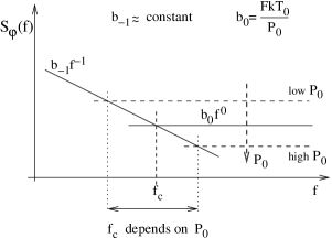
Figure 1: Typical phase noise spectral density of an amplifier.

3.1 White noise

The equivalent noise spectrum density at the amplifier input is $N=FkT_{0}$, where $F$ is the noise figure and $kT_{0}$ is the thermal energy. This type of noise is additive. In the presence of a carrier of power $P_{0}$, the phase noise spectral density is

$$S_{\mathchar 295\relax}(f)=b_{0}f^{0}\leavevmode\nobreak\ \text{(constant)}$$ (5)

with

$$b_{0}=\frac{FkT_{0}}{P_{0}}\leavevmode\nobreak\ .$$ (6)

When amplifiers are cascaded, the noise contribution of each stage is divided by the gain of all the preceding stages (Friis formula [friis44ire]). Accordingly, in most practical cases the total noise is chiefly the noise of the first stage. Of course, this also holds for phase noise.

3.2 Flicker noise

Understanding the close-in noise starts from the bare observation that the output spectrum is of the white type—flat in a wide frequency range—when the carrier power is zero, and that noise shows up close to the carrier only when a sufficiently large carrier power is present at the amplifier output. The obvious consequence is that the close-in flickering results from a parametric effect by which the near-dc flicker noise modulates the carrier in amplitude and phase.

The simplest way to understand the noise up-conversion is to model the amplifier signal as a nonlinear function truncated to the 2nd order

$$v_{o}(t)=a_{1}v_{i}(t)+a_{2}v_{i}^{2}(t)+\ldots\leavevmode\nobreak\ ,$$ (7)

in which the complex input signal

$$v_{i}(t)=V_{i}\,e^{j\omega_{0}t}+n^{\prime}(t)+jn^{\prime\prime}(t)$$ (8)

contains the carrier and the internally generated near-dc noise $n(t)=n^{\prime}(t)+jn^{\prime\prime}(t)$. Rather than being an easy-to-identify voltage or current, $n(t)$ is an abstract random signal that also accounts for the efficiency of the modulation process. Combining (7) and (8) and selecting the terms close to the carrier frequency $\omega_{0}$, we get

$$v_{o}(t) =V_{i}\Bigl{\{}a_{1}+2a_{2}\bigl{[}n^{\prime}(t)+jn^{\prime\prime}(t)\bigr{]}\Bigr{\}}e^{j\omega_{0}t}\leavevmode\nobreak\ .$$ (9)

Hence, the random fluctuations are

$$\alpha(t)=2\>\frac{a_{2}}{a_{1}}\>n^{\prime}(t)\quad\text{and}\quad\mathchar 295\relax(t)=2\>\frac{a_{2}}{a_{1}}\>n^{\prime\prime}(t)\leavevmode\nobreak\ .$$ (10)

Deriving Eq. (10), the statistical properties of $n^{\prime}(t)$ and $n^{\prime\prime}(t)$ are not affected by the carrier power. This accounts for the experimental observation that the amplifier phase noise given in $\mathrm{\,rad^{2}/Hz}$ is about independent of power in a wide range [halford68fcs, walls97uffc, hati03fcs]. Thus

$$S_{\mathchar 295\relax}(f)=b_{-1}f^{-1}\qquad\text{$b_{-1}\approx$ constant}\leavevmode\nobreak\ .$$ (11)

Of course, some dependence on $P_{0}$ remains. We ascribe it to terms of order higher than 2 in (7), and to the effect of the large signal regime on the dc bias. In the case of bipolar amplifiers used in HF/VHF amplifiers, $b_{-1}$ is in the range of $10^{-12}$ to $10^{-14}$ $\mathrm{\,rad^{2}/Hz}$ ($-120$ to $-140$ $\mathrm{\,dBrad^{2}/Hz}$).

When $m$ amplifiers are cascaded, the The Friis formula does not apply. Instead, the phase noise barely adds

$$(b_{-1})_{\text{cascade}}=\sum_{i=1}^{m}(b_{-1})_{i}\leavevmode\nobreak\ .$$ (12)

This occurs because the $1/f$ phase noise is about independent of power. Of course, the amplifiers are supposed independent.

3.3 Phase noise spectrum

Combining white noise [Eq. (5)] and flicker noise [Eq. (11)], there results the spectral density $S_{\mathchar 295\relax}(f)$ shown in Fig. 1. It is important to understand that the white noise term $b_{0}f^{0}$ depends on the carrier power $P_{0}$, while the flicker term $b_{-1}f^{-1}$ does not. Accordingly, the corner frequency $f_{c}$ at which $b_{-1}f^{-1}=b_{0}$ is a function of $P_{0}$, thus $f_{c}$ should not be used to describe noise. The parameters $b_{-1}$, $F$, and $P_{0}$ should be used instead.

4 Phase noise in feedback oscillators

4.1 The Leeson effect

noise-model

Figure 2: Oscillator model and its phase-space equivalent. For the sake of simplicity all the dependence on $s$ is moved to $\beta(s)$, hence the gain $A$ is assumed constant. The scheme emphasizes the amplifier phase noise. Amplitude noise is not considered.

Figure 2 shows a model for the feedback oscillator, and its equivalent in the phase space. All signals are the Laplace transform of the time-domain quantities, as a function of the complex frequency $s=\sigma+j\omega$. The oscillator transfer function is derived from Fig. 2 A according to the basic rules of linear systems

$$H(s)\;=\;\frac{1}{\beta(s)}\>\frac{1}{\dfrac{1}{A\beta(s)}-1}\;=\;\frac{A}{1-A\beta(s)}$$ (13)

Stationary oscillation occurs at the angular frequency $\omega_{0}$ at which $A\beta(j\omega)=1$, thus $|A\beta(j\omega)|=1$ and $\arg[A\beta(j\omega)]=0$. This is known as the Barkhausen condition for oscillation. At $s=j\omega_{0}$ the denominator of $H(s)$ is zero, hence oscillation is sustained with zero input signal. Oscillation starts from noise or from the switch-on transient if $\Re\{A\beta(s)|_{s=j\omega_{0}}\}>1$ (yet only slightly greater than $1$ for practical reasons). When the oscillation reaches a threshold amplitude, the loop gain is reduced to $1$ by saturation. The excess power is pushed into harmonics multiple of $\omega_{0}$, and blocked by the resonator. For this reason, at $\omega_{0}$ the oscillator operates in quasi-linear regime.

In most quartz oscillators, the sustaining amplifier takes the form of a negative resistance that compensates for the resonator loss. Such negative resistance is interpreted (and implemented) as a transconductance amplifier that senses the voltage across the input and feeds a current back to it. Therefore, the negative-resistance oscillator loop is fully equivalent to that shown in Fig. 2.

In 1966, D. B. Leeson [leeson66pieee] suggested that the oscillator phase noise is described by

$$S_{\mathchar 295\relax}(f)=\left[1+\frac{1}{f^{2}}\,\frac{\nu_{0}^{2}}{4Q^{2}}\right]S_{\psi}(f)\qquad\text{(Leeson)}\,,$$ (14)

This formula calls for the phase-space representation of Fig. 2 B, which deserves the following comments.

The Laplace transform of the phase of a sinusoid is probably the most common mathematical tool in the domain of PLLs [klapper-frankle:pll, gardner:pll, best:pll, egan:pll]. Yet it is unusual in the analysis of oscillators. The phase-space representation is interesting in that the phase noise turns into additive noise, and the system becomes linear. The noise-free amplifier barely repeats the input phase, for it shows a gain exactly equal to one, with no error. The resonator transfer function, i.e., the Laplace transform of the impulse response, is

$$B(s)=\frac{1}{1+s\tau}\qquad\tau=\frac{2Q}{\omega_{0}}\leavevmode\nobreak\ .$$ (15)

The inverse time constant is the low-pass cutoff angular frequency of the resonator

$$\omega_{L}=\frac{1}{\tau}=\frac{\omega_{0}}{2Q}\leavevmode\nobreak\ .$$ (16)

The corresponding frequency

$$f_{L}\;=\;\frac{\omega_{L}}{2\pi}\;=\;\frac{1}{2\pi\tau}\;=\;\frac{\nu_{0}}{2Q}$$ (17)

is known as the Leeson frequency. Equation (15) is proved in two steps:

1. Feed a Heaviside step function $\kappa U(t)$ in the argument of the resonator input sinusoid. The latter becomes $\cos\left[\omega_{0}t+\kappa U(t)\right]$.

2. Linearize the system for $\kappa\rightarrow 0$. This is correct in low phase noise conditions, which is certainly our case. Accordingly, the input signal becomes $\cos(\omega_{0}t)-\kappa\sin(\omega_{0}t)U(t)$.

3. Calculate the Laplace transform of the step response, and use the property that the Laplace transform maps the time-domain derivative into a multiplication by the complex frequency $s$. The Dirac function $\delta(t)$ is the derivative of $U(t)$.

The full mathematical details of the proof are available in [rubiola05arxiv-leeson, Chapter 3].

Applying the basic rules of linear systems to Fig. 2 B, we find the transfer function

$$\mathcal{H}(s)\;=\;\frac{\Phi(s)}{\Psi(s)}\;=\;\frac{1}{1-B(s)}\;=\;\frac{1+s\tau}{s\tau}\leavevmode\nobreak\ ,$$ (18)

thus

$$\left|\mathcal{H}(j\omega)\right|^{2}=\frac{1+\omega^{2}\tau^{2}}{\omega^{2}\tau^{2}}\leavevmode\nobreak\ .$$ (19)

The Leeson formula (14) derives from Eq. (19) by replacing

$$\omega=2\pi f\quad\text{and}\quad\tau=\frac{Q}{\pi\nu_{0}}\leavevmode\nobreak\ .$$ (20)

The transfer function $\mathcal{H}(s)$ has a pole in the origin (pure integrator), which explains the Leeson effect, i.e., the phase-to-frequency noise conversion at low Fourier frequencies. At high Fourier frequencies it holds that $\mathcal{H}(j\omega)=1$. In this region, the oscillator noise is barely the noise of the sustaining amplifier.

types

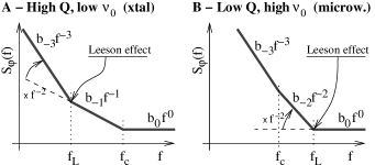
Figure 3: Oscillator phase noise spectra, not accounting for the output buffer.

The amplifier phase noise spectrum contains flicker and white noise, i.e., $S_{\psi}(f)=\left(b_{-1}\right)_{\text{ampli}}f^{-1}+\left(b_{0}\right)_{\text{ampli}}$. Feeding such $S_{\psi}(f)$ into the Leeson formula (14), the oscillator $S_{\mathchar 295\relax}(f)$ can only be one of those shown in Fig. 3. Denoting with $f_{c}$ the corner frequency at which flicker noise equals white noise, we often find $f_{L}<f_{c}$ in HF/VHF high-$Q$ oscillators, and $f_{L}>f_{c}$ in microwave oscillators. In ultra-stable HF quartz oscillators (5–10 MHz), the spectrum is always of the type A ($f_{L}<f_{c}$).

4.2 Output buffer

The phase noise $S_{\psi\,b}(f)$ of the output buffer barely adds to the oscillator phase noise

$$S_{\mathchar 295\relax\,o}(f)=\left[1+\frac{1}{f^{2}}\,\frac{\nu_{0}^{2}}{4Q^{2}}\right]S_{\psi}(f)+S_{\psi\,b}(f)\leavevmode\nobreak\ .$$ (21)

This a consequence of the flicker noise mechanism explained Section 3.2, and inherent in the model of Fig. 2 B.

4.3 Resonator stability

The oscillator frequency follows the random fluctuation of the resonator natural frequency. However complex or tedious the formal proof for this statement can be, the experimentalist is familiar with the fact that the quartz oscillator can be frequency-modulated by a signal of frequency far higher than the Leeson frequency. For example, a 5 MHz oscillator based on a $Q=2{\times}10^{6}$ resonator shows a Leeson frequency of $1.25$ Hz (see Table LABEL:tab:parameters), while it can be modulated by a signal in the kHz region. Additionally, as a matter of fact, the modulation index does not change law from below to beyond the Leeson frequency. This occurs because the modulation input acts on a varactor in series to the quartz, whose capacitance is a part of the motional parameters.

4.4 Other effects

The sustaining amplifier of a quartz oscillator always includes some kind of feedback; often the feedback is used to implement a negative resistance that makes the resonator oscillate by nulling its internal resistance. The input admittance $Y_{i}$ seen at the amplifier input can be represented as

$$Y_{i}=Y_{i}^{(v)}+Y_{i}^{(r)}\leavevmode\nobreak\ ,$$ (22)

that is, the sum of a virtual term $(v)$ plus a real term $(r)$. The difference between ‘virtual’ and ‘real’ is that in the case of the virtual admittance the input current flows into the feedback path, while in the case of the real admittance the input current flows through a grounded dipole. This is exactly the same concept of virtual impedance routinely used in the domain of analog circuits [franco:operational-amplifiers, Chapter 1]. The admittance $\smash{Y_{i}^{(r)}}$ also includes the the effect of the pulling capacitance in series to the resonator, and the stray capacitances of the electrical layout. As a consequence, the fluctuation $\delta\smash{Y_{i}^{(v)}}$ is already accounted for in the amplifier noise, hence in the model of Fig. 2, while the fluctuation $\delta\smash{Y_{i}^{(r)}}$ is not. On the other hand, $\smash{Y_{i}^{(r)}}$ interacts with the resonator parameters, thus $\delta\smash{Y_{i}^{(r)}}$ yields frequency fluctuations not included in the Leeson effect. The hard assumption is made in our analysis, that $|\delta\smash{Y_{i}^{(r)}}|^{2}\ll|\delta\smash{Y_{i}^{(v)}}|^{2}$. In words, we assume that the fluctuation of the electronics are chiefly due to the gain mechanism of the amplifier. Whereas the variety of circuits is such that we can not provide a proof for this hypothesis, common sense suggests that electronics works in this way.