Unitary theory of laser Carrier-Envelope Phase effects

Abstract

We consider a quantum state interacting with a short intense linearly polarized laser pulse. Using the two-dimensional time representation and Floquet picture we establish a straightforward connection between the laser carrier-envelope phase (CEP) and the wave function. This connection is revealed as a unitary transformation in the space of Floquet components. It allows any CEP effect to be interpreted as an interference between the components and to put limits on using the CEP in coherent control. A 2-level system is used to illustrate the theory. On this example we demonstrate strong intensity sensitivity of the CEP effects and predict an effect for pulses much longer than the oscillation period of the carrier.

1 Introduction

Progress in manipulating ultrashort intense laser pulses has made possible studying laser-matter interactions in qualitatively new regimes. For instance, very short pulses having only a few oscillations of the laser field can be produced [1, 2]. In contrast to the more conventional case, when a laser pulse is much longer than the carrier period, the carrier phase of the pulse with respect to the envelope maximum can become an important parameter for short pulses. This phase is called the carrier-envelope (CE) phase (CEP). It has been demonstrated experimentally, that the CE phase can significantly influence ionization of Kr atoms by infrared laser pulses [1]. Recently, similar experiments were performed with Rydberg states of Rb atoms ionized by a few-cycle 25 MHz pulse [3], and the spatial distribution of the ionized electrons has shown sensitivity to the CEP. Even potentially stronger effects were predicted theoretically for dissociation of the HD⁺ in the laser field [4] and experiments are being performed. The sensitivity of high harmonic generation (HHG) on the laser CEP is also known [2]. Molecular isomerisation in short intense laser pulses also provides an interesting example where CEP effects are important [5].

However, the CEP effects are, probably, not fully understood theoretically. Only a few models that go beyond the qualitative picture have been discussed. An interesting interpretation of the CEP effects in ionization as a double-slit interference in the time domain was proposed by F.Linder et al. [6]. This interpretation, however, does not help to describe results for high energy electrons, or, more generally, to describe the dependence of the CEP effects on the final state energy. The goal of this paper is to propose a simple and physically significant interpretation for the influence of the CE phase on the interacting wave function. We propose a picture revealing a simple but exact relationship between the laser phase and the state.

We use the 2D time (or $(t,t^{\prime})$) formalism [7] together with a Floquet representation of the interaction. This approach allows a model-free separation of different time scales present in a short laser pulse. We shall see how the CEP can be eliminated from the equations by a simple unitary transformation. This transformation allows recovery of the CEP dependence of a final state from the wave function components for one CE phase only.

We illustrate our result by demonstrating how the state of a two-level system (a qubit) can be controlled by a short pulse, revealing the mechanisms of CEP influence on the state of the system. We demonstrate and explain dependence of the CEP effect magnitude on the maximal field of the pulse and the pulse duration. It is shown that CEP effects can be observed even for pulses that are much longer than one oscillation period of the carrier.

2 Theory

We base our approach on investigating the time-dependent Schrödinger equation

$$i\frac{\partial}{\partial t}\Psi=[H_{0}+V(t)]\Psi\ .$$ (1)

Here $\Psi$ is the wave function, $H_{0}$ is the Hamiltonian of the system without laser field, and $V(t)$ stands for the laser-matter interaction potential. We shall consider laser-matter interactions of the following form

$$V(t)=-{\bf E}(t)\cdot{\bf d}\cos(\omega t+\varphi)\ \ .$$ (2)

Here ${\bf E}(t)$ is the envelope of the laser pulse field, d is the dipole interaction operator, $\omega$ is the laser carrier frequency and $\varphi$ is the carrier-envelope phase. The latter can be a very important parameter especially for sufficiently short pulses, and it is the main parameter studied in this work.

In what follows, we give a brief description of the 2D time formalism [7] and introduce a two-dimensional time representation for a system in a pulsed laser field. We shall demonstrate how this representation allows eliminating of the CEP $\varphi$ from the evolution equation and construction of a CEP-independent solution. The CEP dependent solution of the initial equation (2) can be recovered from the CEP-independent solution with a unitary transform.

2.1 The 2D time formalism for a system in a periodic external field

The formalism of two-dimensional time is very useful to treat time-dependent systems that show both periodic and non-periodic behavior, such as atoms and molecules in a field of a laser pulse. One of the advantages of this formalism is that it allows separation of periodic and non-periodic dynamics without resorting to adiabatic expansions that might converge slowly for nonadiabatic systems.

In the 2D-time representation one introduces a second time $s$, such that the envelope and the periodic factors in the laser-matter interaction (2) depend on different time coordinates

$$\begin{array}[]{l}V(s,t)=-({\bf E}(s),{\bf d})\cos(\omega t+\varphi)\\ H(s,t)=H_{0}+V(s,t)\ \ \ .\end{array}$$ (3)

One also introduces a second time dynamics

$$(i\frac{\partial}{\partial s}+i\frac{\partial}{\partial t})\Psi(s,t)=(H_{0}+V(s,t;\varphi))\Psi(s,t)\ \ \ .$$ (4)

It is not difficult to see that if $\Psi(s,t)$ satisfies (4), the solution of (1) can be written as $\Psi(t)=\Psi(s,t)\mid_{s=t}$. Indeed, restricting the solution to the “diagonal” time $s=t$ and substituting it to the left-hand side of the equation (1) we get the left-hand side of the equation (4)

$$i\frac{\partial}{\partial t}\Psi(t,t)=(i\frac{\partial}{\partial s}+i\frac{\partial}{\partial t})\Psi(s,t)\mid_{s=t}\ \ \ .$$

The right-hand sides of the equations (1) and (4) are identical at $s=t$. Thus, once the 2D-time equation is solved, one has a solution of the original equation (1) as well. More detailed discussion of the 2D-time formalism can be found at the original paper of Peskin and Moiseev [7].

2.2 Floquet representation for a finite-time pulse

If the laser pulse duration is not considerably shorter than the oscillation period $2\pi/\omega$, expanding the wave function $\Psi(s,t)$ into a Fourier series in $t$ can be a reasonable way of solving equation (4), even for pulse duration comparable with the oscillation period [8]. In fact, this approach holds as far as the description of the laser pulse itself in terms of carrier and envelope is valid [11]. In this paper we discuss pulses longer than one oscillation period, and, thus, our approach to solving equation (4) is justified.

We start constructing the Floquet representation [9, 10] for the laser pulse from expanding the wave function

$$\Psi(s,t)=\sum_{n=-\infty}^{\infty}e^{in\omega t}\phi_{n}(s)\ \ \ .$$ (5)

We shall call the coefficients $\phi_{n}(s)$ $n$-photon emission ($n>0$) and absorption ($n<0$) amplitudes.

Bringing the time derivative $i\frac{\partial}{\partial t}$ to the right hand side of equation (4) and substituting the representation (5) we come up with the following infinite system of equations

$$\begin{array}[]{c}i\frac{\partial}{\partial s}\phi_{n}(s)=\begin{array}[t]{r}\frac{1}{2}e^{i\varphi}({\bf E}(s),{\bf d})\ \phi_{n-1}(s)\\ +(H_{0}+n\omega)\ \phi_{n}(s)\\ +\frac{1}{2}e^{-i\varphi}({\bf E}(s),{\bf d})\ \phi_{n+1}(s)\end{array}\\ n=-\infty,\ldots,-1,0,1,\ldots,\infty\end{array}\ \ \ .$$ (6)

Starting at time $s=s_{-}$ from the initial state

$$\begin{array}[]{lr}\phi_{0}(s_{-})=\psi_{0}\\ \phi_{n}(s_{-})=0&n\neq 0\end{array}$$

and propagating the amplitudes according to (6) sufficiently long, we can investigate different laser-induced processes, such as dissociation, ionization, (de)excitation etc.

It is convenient to introduce a vector of n-photon amplitudes ${\bf\Phi}(s;\varphi)$ and a Floquet Hamiltonian

$${\bf H}(s;\varphi)\equiv{\bf H}_{0}+{\bf V}(s;\varphi)$$

where ${\bf H}_{0}$ stands for the diagonal and ${\bf V}(s;\varphi)$ for the off-diagonal terms in the equation (6). The equation (6) can be written as

$$i\frac{\partial}{\partial s}{\bf\Phi}(s;\varphi)={\bf H}(s;\varphi){\bf\Phi}(s;\varphi)\ \ \ .$$

In this notation we emphasize that the Floquet Hamiltonian and the solution both depend on the carrier-envelope phase $\varphi$. This dependence, however, is parametric, and it can be eliminated.

2.3 Unitary equivalence of the CEP

The obvious advantage of equation (6) for studying the CEP effect is that the phase dependence enters the equation linearly. As we shall see, it allows exclusion of the CE phase from the Floquet Hamiltonian by a simple unitary transformation.

Let us introduce the following operator ${\bf U}(\varphi)$ acting in the n-photon amplitude space

$$[{\bf U}(\varphi)]_{mn}=\delta_{mn}e^{-in\varphi}\ \ \ .$$

Now consider the Floquet Hamiltonian ${\bf H}(0)$corresponding to $\varphi=0$. It is easy to verify that the following relation holds:

$${\bf H}(\varphi)={\bf U^{\dagger}}(\varphi){\bf H}(0){\bf U}(\varphi)\ \ \$$

and to rewrite the evolution equation as

$$i\partial_{s}{\bf U}(\varphi){\bf\phi}(s;\varphi)={\bf H}(0){\bf U}(\varphi){\bf\phi}(s;\varphi)\ \ \ .$$

This equation helps to establish the main result of this paper, which is the unitary equivalence of solutions corresponding to different carrier-envelope phases

$${\bf\Phi}(s;\varphi)={\bf U^{\dagger}}(\varphi){\bf\Phi}(s;0)\ \ \ \ .$$ (7)

This relationship allows any CEP effect to be interpreted as interference of different n-photon channels. It can be clearly seen if we recall the expression for the wave function in physical time

$$\Psi(t;\varphi)=\sum_{n=-\infty}^{\infty}e^{in\varphi}\tilde{\phi}_{n}(t;0)\ \ ,$$ (8)

where we have introduced the final state components of the wave function $\tilde{\phi}_{n}(t;0)=e^{in\omega t}\phi_{n}(t;0)$. After the laser pulse is off at the moment $t=t_{0}$, the components $\tilde{\phi}_{n}$ depend on time uniformly due to the internal dynamics of the system only, i.e. ${\bf\phi}(t)=e^{-i{\bf H}_{0}(t-t_{0})}{\bf\phi}(t_{0})$. Depending on the laser CEP, the wave function components $\tilde{\phi}_{n}$ gain phases proportional to the corresponding net number of exchanged photons $n$ and the CEP $\varphi$.

It is important to note that all the given results are obtained under rather general assumptions of dipole laser-matter interaction and a stable shape of the laser pulse. We did not assume anything specific for any particular physical system. That means that any CEP effect can be considered as interference of several n-photon channels.

2.4 CEP effect observation

Before discussing application of the formula (8) to particular model systems, we say a few words on observing the phase effects in general.

Let $\hat{O}$ be an observable of interest. Using the representation (8) at large times we get an explicit CEP dependence of the mean value of $\hat{O}$ through the n-photon components at zero phase

$$\langle\hat{O}\rangle=\sum_{k,n=-\infty}^{\infty}e^{i(k-n)\varphi}\langle\phi_{n}(t_{0};0)|\hat{O}(t)|\phi_{k}(t_{0};0)\rangle\ \ \ ,$$

where $\hat{O}(t)=e^{i{\bf H}_{0}(t-t0)}\hat{O}e^{-i{\bf H}_{0}(t-t0)}$. Rearranging the terms in the series and using $\hat{O}^{\dagger}=\hat{O}$ we get a Fourier series for the $\langle\hat{O}\rangle$ CEP dependence

$$\langle\hat{O}\rangle(\varphi)=\frac{\alpha_{0}}{2}+\sum_{k=1}^{\infty}({\rm Re}\alpha_{k}\cos k\varphi+{\rm Im}\alpha_{k}\sin k\varphi)\ \ \$$ (9)

with the coefficients $\alpha_{k}$ defined as

$$\alpha_{k}=2\sum_{n=-\infty}^{\infty}\langle\phi_{n-k}(t_{0};0)|\hat{O}(t)|\phi_{n}(t_{0};0)\rangle\ \ \ .$$

It is useful to introduce a measure of CEP effect observability. This measure can be chosen as a norm of the $\varphi$-dependent part in equation (9)

$$\sigma=(\sum_{k=1}^{\infty}|\alpha_{k}|^{2})^{\frac{1}{2}}\ \ \ .$$ (10)

We shall refer to this quantity as absolute CEP amplitude of the observable $\hat{O}$, since it indicates how much $\langle\hat{O}\rangle$ can deviate from its mean value $\alpha_{0}$ when varying the CEP. It is worth mentioning that $\sigma$ is directly connected to the mean square deviation of $\langle\hat{O}\rangle$ from its CEP-averaged value, namely:

$$[\int_{0}^{2\pi}(\langle\hat{O}\rangle(\varphi)-\frac{\alpha_{0}}{2})^{2}d\varphi]^{\frac{1}{2}}=\sqrt{\pi}\sigma\ \ \ .$$

It is also useful to have a CEP amplitude weighted with the mean value $\alpha_{0}$ and experimental sensitivity $\delta$

$$\sigma_{W}=\frac{\sigma}{\frac{\alpha_{0}}{2}+\delta}\ \ \ .$$ (11)

3 Numerical illustrations

In the following section we give two types of demonstrations: quantitative and qualitative.

Quantitatively, we shall check the agreement of equations (7) and (8) with CEP results calculated independently. For that type of demonstration we have to calculate the n-photon amplitudes either from a direct solution of equation (4) or by extracting them from an independently calculated final state wave function. Knowledge of the amplitudes, however, is rather expensive. To predict the CEP response of any particular physical system, we have to know not only the population probabilities of the Floquet states, but their phases as well. Usually, this information can be obtained only from a numerical solution of the TDSE, and we shall explain how expression (8) can be used to reduce the amount of numerical calculations.

Qualitatively, we shall discuss the physical conditions needed to observe CEP effects experimentally. Such conditions are equivalent to the existence of several interfering components. In fact, as equations (7,8) suggest, CEP effects exist if and only if several n-photon components contribute to the same physical state. We shall see how this condition is realized in a simple 2-level model. On this example we shall discuss intensity and pulse duration dependence of the CEP effects. We should mention, however, that not all the physical systems conventionally treated in a 2-level approximation are suitable for clear CEP effect demonstrations. For instance, choosing an experimental realization, one has to fulfill the condition that the two states used in the demonstration must be well separated from other eigenstates of the system, because the important transitions have essentially nonresonant multiphoton character. Such systems can be realized, for example, as double quantum dots [13, 14] or as ionic hyperfine qubits [15]. Although the 2-level model cannot describe processes of ionization or molecular dissociation realistically, it still gives a reasonable qualitative description of the CEP effect observability. More detailed study of the CEP effects involving continuum states is a subject for another investigation.

In all the examples we shall use a Gaussian shape of the laser pulse

$$E(t)=E_{0}e^{-(\frac{t}{\tau})^{2}}\ \ ,$$

$$V(t)=-d\cdot E(t)\equiv V_{0}e^{-(\frac{t}{\tau})^{2}}\ \ ,$$

where $E_{0}$ is the peak field, $\sqrt{2\ln 2}\tau$ is the intensity FWHM pulse duration and $V_{0}\equiv-d\cdot E(T)$ is the peak interaction energy. Since we are particularly interested in molecular systems, we choose energy scales in the typical energy range of molecular vibrational states and fix the laser carrier frequency to 0.058 a.u., what corresponds to a standard 790 nm Ti:Sapphire laser.

3.1 Excitations in a 2-state model.

We start from a simplest example of an excitation in a 2-state system. Let $|a\rangle$ and $|b\rangle$ be the two eigenstates with energies $E_{a}$ and $E_{b}$. Without loss of generality we can set the first energy to zero, $E_{a}\equiv 0$, $E_{b}\equiv E_{a}+\Delta=\Delta$, and consider $|a\rangle$ the initial state. The wave function in this case takes form

$$\psi=a(t;\varphi)|a\rangle+b(t;\varphi)|b\rangle\ \ \ .$$

Suppose the coupling to the laser field between the two states is proportional to the laser field, such that the corresponding time-dependent Scrödinger equation reads

$$i\frac{\partial}{\partial t}\left(\begin{array}[]{c}a(t)\\ b(t)\end{array}\right)=\left(\begin{array}[]{cc}0&V(t)\cos(\omega t+\varphi)\\ V(t)\cos(\omega t+\varphi)&\Delta\end{array}\right)\left(\begin{array}[]{c}a(t)\\ b(t)\end{array}\right)\ .$$ (12)

After introducing the coupling energy $V(t)=-d\cdot E(t)$ and keeping only states coupled to the initial state $|a\rangle$ the Floquet Hamiltonian ${\bf H}$ for $\varphi=0$ in (6) can be written as

$${\bf H}=\left(\begin{array}[]{ccccccc}\ldots&\frac{V(s)}{2}&0&0&0&0&0\\ \frac{V(s)}{2}&0-2\omega&\frac{V(s)}{2}&0&0&0&0\\ 0&\frac{V(s)}{2}&\Delta-\omega&\frac{V(s)}{2}&0&0&0\\ 0&0&\frac{V(s)}{2}&0&\frac{V(s)}{2}&0&0\\ 0&0&0&\frac{V(s)}{2}&\Delta+\omega&\frac{V(s)}{2}&0\\ 0&0&0&0&\frac{V(s)}{2}&0+2\omega&\frac{V(s)}{2}\\ 0&0&0&0&0&\frac{V(s)}{2}&\ldots\end{array}\right)\ \ \ .$$

In this representation even Floquet amplitudes of correspond to the ground state $|a\rangle$ and odd ones to the excited state $|b\rangle$, i.e.

$$\begin{array}[]{l}|\phi_{2n}\rangle\equiv\tilde{a}_{2n}(t)e^{-2n\omega t}|a\rangle\ \ ,\\ |\phi_{2n+1}\rangle\equiv\tilde{b}_{2n+1}(t)e^{-(2n+1)\omega t}|b\rangle\ \ ,\\ n=-\infty,\ldots,\infty\ \ \ .\end{array}$$

Let us demonstrate first how the CEP reveals itself in the excitation probability. At first, we calculate the Floquet amplitudes for $\varphi=0$ numerically. In this example we use the energy gap $\Delta=0.066$ a.u., which slightly exceeds the photon energy, and the dipole coupling is chosen as $d=-1$ a.u. The pulse intensity is chosen as $5\times 10^{14}$ W/cm², which corresponds to the peak interaction energy $V_{0}=0.1194$ a.u., and the pulse duration is $\tau=248$ a.u., which is about 7 fs intensity FWHM. The calculations were performed with 30 Floquet blocks, what guarantees accurate results even for intensities higher than $10^{15}$ W/cm². Let us look for the excitation probability $P_{ex}$ as the observable. We choose the final propagation time $t_{0}=4\tau=992$ a.u., when the field is negligible. According to equation (8), the final state wave function is expressed in terms of the Floquet amplitudes as

$$\begin{array}[]{rcl}\Psi(t;\varphi)&=&\left(\sum_{n=-\infty}^{\infty}e^{i2n\varphi}\tilde{a}_{2n}(t_{0})\right)|a\rangle\\ &+&\left(\sum_{n=-\infty}^{\infty}e^{i(2n+1)\varphi}\tilde{b}_{2n+1}(t_{0})\right)e^{-\Delta(t-t_{0})}|b\rangle\ \ .\end{array}$$ (13)

Thus, in order to calculate the excitation probability we have to evaluate the odd n-photon components of the final state

$$P_{ex}=|\langle b|\Psi\rangle|^{2}=|\sum_{n=-\infty}^{\infty}e^{i(2n+1)\varphi}\tilde{b}_{2n+1}(t_{0})|^{2}\\$$

The following final state amplitudes will contribute to the excited state of the system at the final time $\tilde{b}_{1}(4\tau;0)=0.0092-0.0202i$, $\tilde{b}_{-1}(4\tau;0)=0.1445-0.3178i$, $\tilde{b}_{-3}(4\tau;0)=-0.0543+0.1193i$. All other amplitudes are negligibly small. According to equation (13), the excited state component CEP dependence reads

$$b(t;\varphi)|b\rangle=(\tilde{b}_{1}e^{i\varphi}+\tilde{b}_{-1}e^{-i\varphi}+\tilde{b}_{-3}e^{-3i\varphi})e^{-i\Delta(t-t_{0})}|b\rangle\ \ \ .$$

This results in the following explicit expression for the excitation probability:

$$P_{ex}=0.1395-0.07602\cos 2\varphi-0.00582\cos 4\varphi\ \ .$$

This line is shown in the Fig. 1 together with results of direct solution of equation (12). Since no approximations were made, besides cutting off the series (13), the perfect agreement is not surprising.

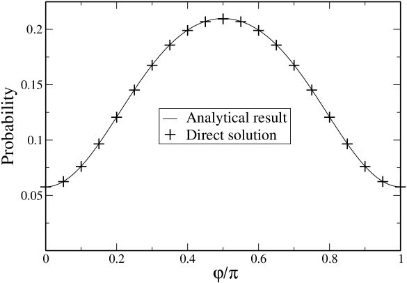
Figure 1: 2-level system photoexcitation probability as a function of the CEP for the energy gap $\Delta=0.066$ a.u., laser frequency $\omega=0.058$ a.u., peak field $V_{0}=0.1194$ a.u., pulse duration $\tau=248$ a.u.. The dots are obtained from the direct solution of equation (12), the line is constructed from the final state n-photon amplitudes for $\varphi=0$.

Giving this example, we calculated the Floquet amplitudes by direct solution of the system of equations (6). In practical applications, however, this approach is not effective: usually, solving a small system $n$ times is simpler than solving an $n$ times bigger system of equations once. In the case of the equations (6) the situation is even worse. Even if we have only 3 components contributing to the final state, as in our example, one needs more than 5 Floquet blocks kept in the equations to reproduce the correct dynamics even for moderate peak fields. Because of that, recovering the amplitudes by subsequently solving the original Schrödinger equations directly for several CE phases and fitting the expression (8) to the wave function should be a much more effective procedure for realistic calculations.

After giving this numerical example, we are ready to discuss some qualitative properties of the CEP effects. Are there any conditions for the peak interaction energy $V_{0}$ and the pulse duration $\tau$ that limit an observability of CEP effects?

Let us discuss the intensity dependence first. In order to have interference, one has to make sure that there are several $n$-photon components contributing to the states with the same final state energy. It cannot be achieved with one-photon transitions only, so there must be a minimal intensity that allows a clear observation of the CEP effect. To understand the lower intensity limit, consider the eigenvalues of ${\bf H}$ shown in Fig. 2. On the leading edge of the laser pulse the interaction energy grows up, this correponds to moving from the left to the right in Fig. 2. After the peak, which defines the rightmost point in Fig. 2, the system goes from the right to the left during the trailing edge of the pulse.

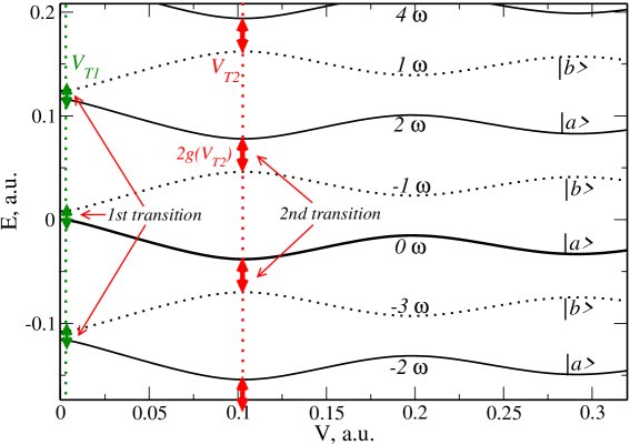
Figure 2: 2-level system Floquet Hamiltonian eigenstates as a function of the laser-matter interaction energy $V=-E\cdot d$. The model parameters are $\omega=0.058$a.u., $\Delta=0.066$a.u. Thick lines correspond to the ground state and dotted lines to the excited state.

As one can see from tracking the eigenvalues of the dressed system, the two crossings that we need to populate the state $|b\rangle$ via 1- and 3-photon transitions correspond to the interaction energies $V_{T1}\approx 0$ a.u. and $V_{T2}\approx 0.1$ a.u.. This gives us a limitation on the laser peak intensity: no interference can happen if the maximal field-matter interaction energy does not approach the second crossing. We can safely say that in our example no CEP effect is expected if the peak interaction energy is smaller than $0.05$ a.u.. This observation is illustrated in Fig. 3, where we have plotted the weighted CEP effect amplitude (11). As we expected, we see an essential growth of the CEP effect contrast only above $0.05$ a.u., when the peak field starts approaching the 3-photon crossing.

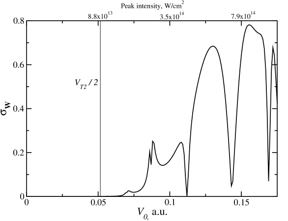
Figure 3: The weighted excitation probability CEP amplitude $\sigma_{W}$ (11) as a function of the peak interaction energy. No phase dependence below $V_{0}=0.05$ a.u. is observed. Calculations were performed with 30 Floquet blocks, the sensitivity parameter $\delta$ in (11) is set to $0.01$.

The big maximal intensity alone, however, is not enough to observe the effect: the field should change fast enough when passing through both crossings, otherwise transition happens adiabatically, and no population transfer occurs. The proper timing conditions must be satisfied. This leads us to the question of the pulse duration dependence of the CEP effects.

As we have seen, nonadiabatic second transition (see Fig. 2) is a necessary condition for the CEP observation. We can use the Landau-Zener model to qualify the presence of the CEP effects by estimating the second transition probability as a function of the pulse duration. Let $V_{T2}$ be the position of the second crossing. For the energy gap of our example ($\Delta=0.066$ a.u.) the level splitting is about $g(V_{T2})=0.016$ a.u. The growth rate of the interaction energy when crossing the second transition region

$$\frac{dV}{dt}=2\frac{V_{T2}}{\tau}\sqrt{\ln\frac{V_{0}}{V_{T2}}}$$

plays the role of velocity in the Landau-Zener formula. Now we are ready to estimate the second transition probability as

$$\begin{array}[]{rcl}P_{2}&=&e^{-2\pi\delta}(1-e^{-2\pi\delta})\\ \delta&=&\frac{g(V_{T2})^{2}\tau}{2V_{T2}\sqrt{\ln(V_{0}/V_{T2})}}\\ \end{array}$$ (14)

If no higher order transitions happen, the amplitude of the CEP effect should be proportional to the square root of this probability, since it is proportional to the amplitude rather than the probability of the m-photon state population. This square root of the probability is shown in Fig. 4a together with the amplitude of the excitation probability CEP dependence. It is clear that probability (14) should have a substantial value to make possible an observation of the CEP effects. Equation (14) shows that CEP effects should disappear exponentially with growing pulse length.

It is important to mention that the pulse duration needed to observe the CEP effects is a property of the laser-matter interaction rather than the laser pulse alone. In the two-level model, as equation (14) suggests, it is defined by level splitting at the second crossing point and the position of the second crossing. For large energy gaps it is easy to obtain smaller multiphoton splitting. This allows one to predict the CEP effects even for pulses that are substantially longer than one oscillation period, as demonstrated in Fig. 4b. There we show the CEP observability $\sigma$ together with its Landau-Zener estimation. Even for pulses longer than $\tau=1700$ a.u., what is about 30 periods in the field FWHM, we still can see a variation of the probability with the CEP about 10%.

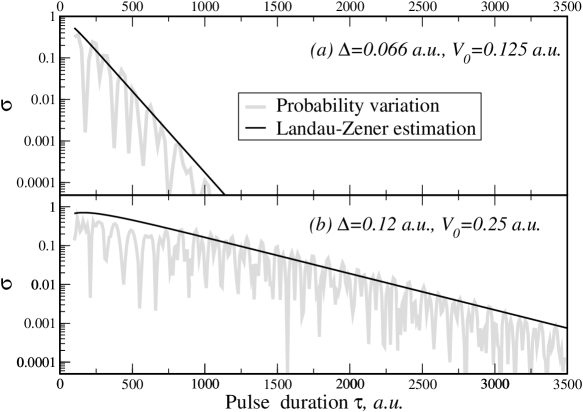
Figure 4: CEP variation of the excitation probability as a function of the pulse duration. The black lines correspond to the Landau-Zener estimation of the effect via the transition probability at the second crossing. a) $\Delta=0.066$ a.u. b) $\Delta=0.12$ a.u. The peak interaction energy is taken about 30% higher than the second transition energy.

We must mention, however, that experimental observability of the long-pulse effect can be limited by the stability of the pulse shape, which might be difficult to keep at a time scale smaller than one oscillation period for long pulses.

4 Summary

We have investigated a quantum state experiencing a laser pulse of a stable envelope shape and varying CEP of the oscillatory part. We have shown how the CEP can be excluded from evolution equations and how the CEP dependence of the final state can be recovered from CEP-independent results. On the example of a 2-level system we have demonstrated a critical intensity and pulse duration dependence of CEP effects. In contrast to the common conception that CEP effects can be expected only when the pulse duration is nearly as short as the laser oscillation period, we have demonstrated that CEP effects can exist even for pulses much longer than that. The pulse duration that allows the CEP effect observation critically depends on the properties of the system interacting with a laser pulse. In the 2-level system, long-pulse CEP effects can be observed in essentially above-threshold excitation regimes, when the energy gap is considerably larger than the photon energy.

The approach which is suggested in this paper is rather general, and it would be interesting to study more complex systems from this point of view. For instance, it would be interesting to study how $n$-photon component interference affects high-harmonic generation, ionization and dissociation in different systems. There are also many physical and mathematical questions to be addressed, such as gauge-invariant formulation of the theory and checking the classical limits of the interference effect.

References

- [1] G.G. Paulus, et al., Nature 414, 182 (2001).
- [2] A. Baltuska, et al., Nature 421, 611 (2003).
- [3] A. Gurtler, F. Robicheaux, W. J. van der Zande, and L. D. Noordam, Phys. Rev. Lett 92, 033002 (2004).
- [4] V. Roudnev, B. D. Esry, and I. Ben-Itzhak, Phys. Rev. Lett. 93, 163601 (2004).
- [5] Christoph Uiberacker and Werner Jakubetz, J. Chem. Phys. 120 11532 (2004).
- [6] F. Linder et al., Phys. Rev. Lett, 95 040401, (2005).
- [7] Uri Peskin and Nimrod Moiseev, J.Chem. Phys, 99, 4590 (1993).
- [8] Mikhail V. Korolkov, Burkhard Schmidt, Comp. Phys. Comm. 161, 1-17 (2004).
- [9] Jon H. Shirley, Phys. Rev., 138 B979 (1965).
- [10] Shih-I Chu, Dmitry A. Telnov, Phys. Rep. 390 1 (2004)
- [11] T. Brabec, and F. Krausz, Rev. Mod. Phys. 72, 545 (2000)
- [12] T.T. Nguyen-Dang, C. Lefebvre, H.Abou-Rachid, and O.Atabek, Phys. Rev. A 71 023403 (2005)
- [13] Tobias Brandes, Phys. Rep. 408 315 (2005).
- [14] J.R. Petta, A.C. Johnson, C.M. Marcus, M.P. Hanson, and A.C. Gossard, Phys. Rev. Lett. 93, 186802 (2004).
- [15] B. B. Blinov, D. Leibfried, C. Monroe, and D. J. Wineland, Quant. Inf. Proc. 3 45 (2004).