Anderson Localization of Polar Eigenmodes in Random Planar Composites

Abstract

Anderson localization of classical waves in disordered media is a fundamental physical phenomenon that has attracted attention in the past three decades. More recently, localization of polar excitations in nanostructured metal-dielectric films (also known as random planar composite) has been subject of intense studies. Potential applications of planar composites include local near-field microscopy and spectroscopy. A number of previous studies have relied on the quasistatic approximation and a direct analogy with localization of electrons in disordered solids. Here I consider the localization problem without the quasistatic approximation. I show that localization of polar excitations is characterized by algebraic rather than by exponential spatial confinement. This result is also valid in two and three dimensions. I also show that the previously used localization criterion based on the gyration radius of eigenmodes is inconsistent with both exponential and algebraic localization. An alternative criterion based on the dipole participation number is proposed. Numerical demonstration of a localization-delocalization transition is given. Finally, it is shown that, contrary to the previous belief, localized modes can be effectively coupled to running waves.

1 Introduction

Anderson localization (AL) of classical waves in disordered systems is a fundamental physical phenomenon which takes place in the limit of strong resonant scattering when the “photon mean free path” becomes the order of or less than one wavelength (the Ioffe-Regel criterion) [1]. At a formal level, AL of electromagnetic or acoustic waves is similar to localization of electrons in disordered solids. There are, however, substantial physical differences. One such difference is that the motion of electrons can be finite. In contrast, classical waves can not be, in principle, indefinitely confined in a finite spatial region. In the case of electrons, one of the most important physical manifestations of AL (at zero temperature) is the conductor-insulator transition [2]. Localization of classical waves is manifested differently. If we consider an experiment in which classical waves are transmitted through a disordered slab, an analog of conductivity is the transmission coefficient. Assuming that the slab material is non-absorbing, the transmission coefficient can never turn to zero. However, if the waves are localized in the slab, the transmitted and reflected fields exhibit spatial variations at macroscopic scales (much larger than the wavelength) which are sample-specific (not self-averaging). Emission by localized modes in random positive-gain media is the basis for operation of random lasers [3]. Thus, the common feature of localized states of both electrons and classical waves is that the propagation can not be described by the Boltzmann transport equation or the diffusion approximation to the former.

This paper is focused on AL of electromagnetic waves in a random structure which is distinctly different from either two-dimensional or three-dimensional random media. Namely, we will consider random planar composites (RPCs) [4]. The RPCs are made of small three-dimensional scatterers which are randomly distributed in a thin planar layer. Thus, the electromagnetic interaction in this system is essentially three-dimensional while the geometry is two-dimensional. The RPCs have attracted considerable recent attention due to the variety of potential applications, including surface-enhanced Raman spectroscopy of proteins [5, 6, 7]. The physical implication of AL of electromagnetic waves in RPCs can be best understood by considering an experiment in which the sample is excited by a near-field probe. If the electromagnetic states in the sample are strongly localized (at the particular electromagnetic frequency), the surface plasmon induced by the tip will also be localized and not spread over the entire sample. It must be emphasized, however, that there are other mechanisms that can lead to spatial exponential decay of surface plasmons. This includes decay due to absorption (Ohmic losses in the material and

The localization-delocalization transition is expected to play a crucial role in the near-field tomographic imaging techniques of Refs. [8, 9]. If the states are localized, each near-field measurements will be sensitive only to the local environment of the the tip, while in the opposite case, it would be sensitive to the structure of the sample far away from the tip. The relation between AL and transport of surface plasmons is discussed in detail in Section 3.

The possibility and nature of AL of electromagnetic excitations in the RPCs have been investigated theoretically and numerically [4, 10]. While the conclusions given in these two references are somewhat conflicting, the respective theoretical approaches share some common features. Most importantly, localization of the SP eigenmodes was studied in the quasistatic approximation. However, AL is, essentially, an interference phenomenon [1]. Therefore, account of retardation is essential for its proper understanding. Second, a definition of localization length of a mode based on its “radius of gyration” was adopted in Refs. [4, 10]. Here I argue that this definition, as well as the one based on radiative quality factor (mode lifetime) [11, 12] can not be applied to the electromagnetic localization problem in the RPCs.

Below, I discuss a number of important points concerning AL of classical waves, some of which are applicable only to the RPCs and some are more general. I also provide a numerical demonstration of the Anderson transition in the RPCs. To this end, I use a simple but physically relevant model of small spherical inclusions of diameter $D$ embedded in a transparent dielectric host medium and randomly distributed in a plane inside an $L\times L$ box. Essentially, this is the model used in Refs. [11, 12]. However, I work in a different physical regime and use a different definition for localization. Most of the numerical examples shown below were obtained in the limit $D\ll\ell\ll\lambda\ll L$, where $\ell$ is the average inter-particle distance and $\lambda$ is the wavelength.

2 Physical Model

Consider an infinite transparent dielectric host with $N$ small identical spherical inclusions of diameter $D$ randomly distributed in an $L\times L$ box in the $xy$-plane. The inclusions interact with a plane linearly-polarized electromagnetic wave with the wave number $k=n\omega/c=2\pi/\lambda$, where $n$ is the host index of refraction, $\omega$ is the electromagnetic frequency. We assume that $\lambda\gg D$, but the relation between $\lambda$ and $L$ is arbitrary. Thus, we do not use the quasistatic approximation. However, we do use the dipole approximation which is accurate in the limit of small density of inclusions and $D\ll\lambda$. Assuming that the inclusions are non-magnetic, the electric dipole moments ${\bf d}_{i}$ ($i=1,\ldots,N$) induced in each spherical inclusion satisfy the coupled-dipole equation

$${\bf d}_{i}=\alpha\left[{\bf E}_{\rm inc}\exp(i{\bf k}_{\rm inc}\cdot{\bf r}_{i})+\sum_{j\neq i}G({\bf r}_{i},{\bf r}_{j}){\bf d}_{j}\right]\ ,$$ (1)

where ${\bf E}_{\rm inc}$ is the amplitude of the incident wave, $|{\bf k}_{\rm inc}|=k$, $\alpha$ is the polarizability of inclusion, ${\bf r}_{i}$ is the radius-vector of the $i$-th inclusion and $G({\bf r}_{i},{\bf r}_{j})$ is the dyadic Green’s function for the electric field in a homogeneous infinite host medium given by

$$G({\bf r}_{i},{\bf r}_{j})=k^{3}\left[A(kr_{ij})I+B(kr_{ij})\hat{\bf r}_{ij}\otimes\hat{\bf r}_{ij}\right]\ ,$$ (2)

$$A(x)=[x^{-1}+ix^{-2}-x^{-3}]\exp(ix)\ ,$$ (3)

$$B(x)=[-x^{-1}-3ix^{-2}+3x^{-3}]\exp(ix)\ .$$ (4)

Here $I$ is the unit dyadic, ${\bf r}_{ij}={\bf r}_{j}-{\bf r}_{i}$, $r_{ij}=|{\bf r}_{ij}|$, $\hat{\bf r}_{ij}={\bf r}_{ij}/r_{ij}$ and $\otimes$ denotes tensor product.

The system of equation (1) can be written in operator form as

$$|d\rangle=\alpha(|E_{\rm inc}\rangle+W|d\rangle)\ .$$ (5)

Here the Cartesian components of all dipole moments are given by $d_{i,\sigma}=\langle i,\sigma|d\rangle$, where $i=1,\ldots,N$ and $\sigma=x,y,z$. The above relation defines the orthonormal basis $|i,\sigma\rangle$.

The $3N$-dimensional matrix $W$ is complex symmetric and, hence, non-Hermitian. Since such matrices are not very common in physics, a brief review of their spectral properties is adduced. Eigenvalues of complex symmetric matrices are, generally, complex. The eigenvectors form a complete (but not orthonormal) basis unless the matrix is defective. A matrix is defective if one of its eigenvectors is quasi-null, e.g, its dot product with itself (without complex conjugation) is zero (see below). The geometric multiplicity of a defective matrix is less than its algebraic multiplicity. Non-degenerate symmetric matrices are all non-defective. A matrix can be defective as a result of random degeneracy. The probability of such event is, however, vanishingly small. Below, we assume that $W$ is non-defective, which was the case in all numerical simulations shown below. Further, let $|a\rangle$ and $|b\rangle$ be two distinct eigenvectors of $W$ with components $\langle n|a\rangle=a_{n}$ and $\langle n|b\rangle=b_{n}$. The usual orthogonality condition $\langle a|b\rangle=0$ is replaced by

$$\sum_{n}a_{n}b_{n}\equiv\langle\bar{a}|b\rangle=0\ .$$ (6)

Note that the bilinear form in the above formula is defined without complex conjugation. Such forms are called quasi-scalar products and are denoted by $\langle\bar{a}|b\rangle$, in contrast to the true scalar product $\langle a|b\rangle$. The quasi-scalar product of a vector with itself, $\langle\bar{a}|a\rangle$ is, generally, a complex number, possibly zero. A vector whose quasi-scalar product with itself is zero is called quasi-null. At the same time, each eigenvector (including quasi-null vectors) can be normalized in the usual way, so that $\langle a|a\rangle=1$.

Let $w_{n}$ and $|\psi_{n}\rangle$ be the set of $3N$ eigenvalues and eigenvectors of $W$. We assume here that $|\psi_{n}\rangle$ are normalized so that $\langle\psi_{n}|\psi_{n}\rangle=1$. However, the quasi-scalar product $\langle\psi_{n}|\psi_{n}\rangle$ is, in general, a complex number. We can use the orthogonality rule (6) to obtain the spectral solution to (5):

$$|d\rangle=\sum_{n}{{|\psi_{n}\rangle\langle\bar{\psi_{n}}|E_{\rm inc}\rangle}\over{\langle\bar{\psi_{n}}|\psi_{n}\rangle(z-w_{n})}}\ ,$$ (7)

where $z=1/\alpha$. We note that this spectral solution has been obtained assuming there are no quasi-null eigenvectors. In the opposite case, spectral solution can not be obtained.

For non-absorbing inclusions, ${\rm Im}z=-2k^{3}/3$. This equality can be readily obtained by observing that the extinction cross section $\sigma_{e}=4\pi k{\rm Im}\alpha$ and the scattering cross section $\sigma_{s}=(8\pi k^{4}/3)|\alpha|^{2}$ must be equal in the absence of absorption [13] ($\alpha=1/z$). Analogously, in the case of finite absorption, we have ${\rm Im}z<-2k^{3}/3$. Consequently, energy conservation requires [14] that ${\rm Im}w_{n}\geq-2k^{3}/3$. The eigenstates with ${\rm Im}w_{n}=-2k^{3}/3$ are non-radiating  while the eigenstates with ${\rm Im}w_{n}\sim N(2k^{3}/3)>0$ are super-radiating. The radiative quality factor of the mode is defined as $Q_{n}=1/\gamma_{n}$, $\gamma_{n}={\rm Im}[w_{n}/(2k^{3}/3)]+1$. For a non-radiating state, $\gamma_{n}\rightarrow 0$ and $Q_{n}\rightarrow\infty$. The coupling constant $f_{n}$ for the $n$-th mode is defined as $f_{n}=\langle E_{\rm inc}|\psi_{n}\rangle\langle\bar{\psi}_{n}|E_{\rm inc}\rangle[|{\bf E}_{\rm inc}|^{2}\langle\bar{\psi}_{n}|\psi_{n}\rangle]^{-1}$; the $f_{n}$’s satisfy the sum rule $\sum_{n}f_{n}=N$.

3 The Concept of Anderson Localized for Polar Eigenmodes

In this Section I discuss in more detail the concept of AL of polar eigenmodes and the relation between localization and transport properties. In particular, a rationale is given for studying spatial properties of the eigenmodes which depend only on the sample geometry but not on the material properties of the host medium or inclusions.

It is well known that the electromagnetic problem of two-component composites, if solved within the quasistatics, allows for an effective separation of material properties of the constituents and the geometry of the composite. This idea goes back to the Bergman-Milton spectral theory of composites [15] and has been used in many different settings. For example, dipolar (more generally, multipolar) excitations in aggregated spheres were studied in the 1980-ies by Fuchs, Claro and co-authors [16, 17, 18] using the spectral approach analogous to the Bergman-Milton spectral theory of composites.

I have extended the quasistatic spectral theory of Refs. [15, 16, 17, 18] to the case of samples which are not small compared to the wavelength, e.g., when the effects of retardation are important in Refs. [14, 19]. In this case, similarly to the quasistatics, electromagnetic eigenstates of a two-component mixture or composite can be defined. These eigenstates turn out to be independent of the material properties of the constituents, but, unlike in the quasistatic limit, depend explicitly on $k=\omega/c$. Yet, at a fixed electromagnetic frequency $\omega$, the spatial properties of the eigenstates can be studied irrespectively of the material properties of the constituents. In particular, one can argue that in extended systems the eigenstates can be either localized on several inclusions or delocalized over the whole sample, completely independently of the material properties. This was the point of view taken in Refs. [4, 10].

The connection between propagation of surface plasmon excitations in the system and the localization properties of the eigenstates can be established by examining the spectral solution (7) for the case of local excitation (e.g., by a near-field tip) at the site ${\bf r}_{1}$. If the point of observation is located at the site ${\bf r}_{2}$ (e.g., another near-field tip operating in the collection regime), the amplitude of the measured signal is proportional to the following Green’s function:

$${\mathcal{D}}({\bf r}_{2},{\bf r}_{1})=\sum_{n}\frac{f_{n}({\bf r}_{2},{\bf r}_{1})}{z-w_{n}}\ ,$$ (8)

where

$$f_{n}({\bf r}_{2},{\bf r}_{1})=\frac{\langle{\bf r}_{2}|\psi_{n}\rangle\langle\bar{\psi}_{n}|{\bf r}_{1}\rangle}{\langle\bar{\psi}_{n}|\psi_{n}\rangle}\ .$$ (9)

Let us assume that at a given electromagnetic frequency $\omega$ there are resonance modes, e.g., such mode that ${\rm Re}[z(\omega)-w_{n}(\omega)]\approx 0$. This is, obviously, not always the case, and the above condition depends, in particular, on the material properties of the medium. However, if the resonance excitation of the system is, in principle, possible, summation in (8) can be restricted to resonant modes. In this case, propagation of surface plasmons in the system is governed by the spatial dependence of the functions $f_{n}({\bf r}_{2},{\bf r}_{1})$, where $n$ indexes only resonant modes.

In a strictly periodic infinite system, all eigenmodes are delocalized plane waves, which follows from general symmetry considerations. These delocalized modes form a truly continuous spectrum and can be labeled by a continuous index $q$, where $q$ is the wave vector in the first Brillouin zone of the lattice (here the dimension of $q$ is not specified). Note that the eigenmodes that belong to the continuous spectrum are non-normalizable in the usual sense. This means that the scalar product $\langle\psi_{q}|\psi_{q}\rangle$ does not exists. Instead, the usual delta-function normalization $\langle\psi_{q}|\psi_{q^{\prime}}\rangle=\delta(q-q^{\prime})$ must be used. Obviously, functions $f_{q}({\bf r}_{2},{\bf r}_{1})$ that correspond to the delocalized eigenstates are non-decaying as the distance between the points ${\bf r}_{1}$ and ${\bf r}_{2}$ increases.

At this point, two important comments must be made. First, the fact that the the eigenmodes $|\psi_{q}\rangle$ are delocalized plane waves and the corresponding functions $f_{q}({\bf r}_{2},{\bf r}_{1})$ are non-decaying does not necessarily imply that there can be no exponential spatial decay of surface plasmon excitations in the system. This will be illustrated later in this Section with several examples. Second, eigenvalues in a strictly periodic and non-chiral system are invariant with respect to the change $q\rightarrow-q$ and, therefore, doubly degenerate. This does not lead to defectiveness of the operator $W$ but the degenerate modes must be appropriately orthogonalized.

If we now introduce disorder and break the translational symmetry of an infinite sample, the eigenmodes $|\psi_{n}\rangle$ are no longer plane waves. Still, the modes can be either localized or delocalized. The fundamental property of localized modes is that such modes are square integrable in the sense that $\langle\psi_{n}|\psi_{n}\rangle<\infty$ (in fact, localized modes can always be normalized so that $\langle\psi_{n}|\psi_{n}\rangle=1$) and, therefore, belong to a discrete spectrum. There are two consequences of this fact. First, a localized mode can be characterized by a “center of mass” or a point near which it is localized, which we denote by ${\bf R}$. Second, localized modes can be labeled by a countable index. It is natural to use ${\bf R}$ itself as a label. Let all resonant modes be localized. Then the Green’s function (8) can be written as

$${\mathcal{D}}({\bf r}_{2},{\bf r}_{1})=\sum_{{\bf R}}\frac{f_{{\bf R}}({\bf r}_{2},{\bf r}_{1})}{z-w_{n}}\ ,$$ (10)

where summation is extended over resonant modes localized near the point ${\bf R}$. It is clear from inspection of Eq. (10) and the definition (9) that the above Green’s function is spatially decaying when $|{\bf r}_{1}-{\bf r}_{2}|\rightarrow\infty$, and that the rate of this decay depends on the spatial decay of the eigenmodes.

However, it can be readily seen that the spatial decay of localized eigenmodes does not need to be exponential. This is because the essential requirement of localization $\langle\psi_{n}|\psi_{n}\rangle<\infty$ can be satisfied even if the decay is algebraic. More specifically, it is sufficient that $\psi_{\bf R}({\bf r})=\langle{\bf r}|\psi_{{\bf R}}\rangle$ decays faster than $1/|{\bf r}-{\bf R}|^{d/2}$, where $d$ is the dimensionality of the sample. Accordingly, the spatial decay of the Green’s function (10) can be slower than exponential. In fact, I argue in this paper that electromagnetic eigenstates can not be localized exponentially. This is a consequence of algebraic decay of the free-space Green’s function (2) in a transparent host medium. More specifically, if $|\psi_{n}\rangle$ is an exponentially localized eigenstate, the equation $W|\psi_{n}\rangle=w_{n}|\psi_{n}\rangle$ can not be satisfied due to the fact that $\langle{\bf r}|W|\psi_{n}\rangle$ is asymptotically algebraic and $\langle{\bf r}|\psi_{n}\rangle$ is asymptotically exponential. The impossibility of exponential localization of electromagnetic eigenmodes can be also viewed as a consequence of the fact that there are no bound states for light.

The above arguments apply to infinite samples. However, any numerical computation is restricted to finite systems. Modes of a finite system are always discrete and have a finite $L_{2}$ norm. The difference between the modes which remain discrete in the thermodynamic limit and the modes that become delocalized is then revealed by examining the rate at which these modes decay. The amplitudes of localized modes decay (away from their “center of mass” ${\bf R}$) faster than $1/|{\bf r}-{\bf R}|^{d/2}$. Consequently, a localized mode centered at a point ${\bf R}$ which is sufficiently far from the sample boundaries is insensitive to any change in the sample overall size or shape. In contrast, delocalized modes always remain sensitive to the exact shape of the boundaries. For example, a delocalized mode would change substantially if the system overall size is doubled while a localized mode will be insensitive to such change, as along as it is centered sufficiently far from the original boundaries.

In light of the above, it is interesting to examine the applicability of a localization criterion which based on the eigenmode gyration radius, $\xi_{n}$ (defined in Section 5 below). This parameter was used in Refs. [4, 10] within the quasistatic approximation. An eigenmode was considered to be localized if $\xi_{n}\ll L$, where $L$ is the sample characteristic size. The above inequality was claimed to be a consequence of exponential localization. First, we note that the condition $\xi_{n}\ll L$ is not equivalent to (actually, is weaker than) exponential localization of the eigenmode. As is shown in Section 5 below, it is sufficient that the eigenstate exhibits spatial decay faster than $1/r^{d/2+1}$ for the above inequality to hold. But more importantly, application of this criterion can lead to a grossly inaccurate conclusion about delocalization of an eigenstate when it is, in fact, strongly localized. The reason for this is numerical. Indeed, even though localized eigenstates belong to a countable discrete spectrum, the spacings between eigenvalues $w_{n}$ can be arbitrarily small and tend to decrease with the sample size. Thus, two localized eigenstates with centered at different points ${\bf R}_{1}$ and ${\bf R}_{2}$ can have very close eigenvalues $w_{1}\approx w_{2}$. Numerically, these two eigenstates are quasi-degenerate. That means that any linear superposition of these two eigenstates is also an eigenstate (within numerical precision of the computer). Namely, if $|\psi_{{\bf R}_{1}}\rangle$ and $|\psi_{{\bf R}_{2}}\rangle$ are two quasi-degenerate eigenstates, then the linear combinations

$$|\psi_{\pm}\rangle=\frac{1}{\sqrt{2}}(|\psi_{{\bf R}_{1}}\rangle\pm|\psi_{{\bf R}_{2}}\rangle)$$

are also eigenstates (within the numerical precision). But the gyration radii of $|\psi_{{\bf R}_{1}}\rangle$, $|\psi_{{\bf R}_{2}}\rangle$, on one hand, and of $|\psi_{{\bf r}_{\pm}}\rangle$, on the other, might be very different. Thus, if the first two states are localized with gyration radii $\xi_{1},\xi_{2}\ll L$, the gyration radii of the eigenmodes $|\psi_{{\bf r}_{\pm}}\rangle$ can be of the order of $|{\bf R}_{1}-{\bf R}_{2}|\sim L$. I argue below that a more reliable numerical criterion of localization can be based on the so-called participation number.

Thus, we have established that geometrical properties of electromagnetic eigenmodes play a fundamental role in AL. These eigenmodes are completely defined by the sample geometry and are independent of the material properties, as long as there is no more than two constituents in the medium. Therefore, following Refs. [4, 10] we focus on the properties of the eigenmodes and do not consider a specific material- and frequency-dependent model for the spectral parameter $z$. It should be noted, however, that polarization or electric field can be exponentially confined in space due to several reasons other than AL. The physical phenomena that lead to such confinement can strongly depend on material properties of the medium and should not be confused with AL. In the remainder of this Section, we briefly review several such phenomena.

The first relevant example is exponential decay of evanescent waves. Evanescent decay can lead, for example, to exponential confinement of waves in one-dimensional periodic layered media (photonic crystals). However, evanescent waves are exponentially localized only in one selected direction and are oscillatory in any direction orthogonal to the former.

The second example is decay due to dissipation. It is well known that a superposition of perfectly delocalized states can result in an exponentially decaying wave. Consider a superposition of one-dimensional waves with continuous wave-numbers $q$ (e.g., in a one-dimensional periodic system):

$$d(x)=\int_{-\pi/h}^{\pi/h}\frac{hdq}{2\pi}\frac{e^{iqx}}{z-w(q)}$$ (11)

This equation would describe, for example, propagation of a surface plasmon along a linear periodic chain of nanospheres of period $h$ and integration is extended over the first Brillouin zone of the lattice [20]. It can be shown exactly [21] that for $q>k=\omega/c$, ${\rm Im}w(q)=-2k^{3}/3$. (This is known as the light-cone condition; SP is not coupled to running waves because momentum of the photon can not be conserved. Due to the same reason, a propagating SP with $q>k$ does not radiate.) We now make the usual quasi-particle pole approximation, namely

$$w(q)\approx{\rm Re}w(q_{0})+(q-q_{0})\left|\frac{\partial{\rm Re}w(q)}{\partial q}\right|_{q=q_{0}}-i\frac{2k^{3}}{3}\ ,$$ (12)

where $q_{0}$ is, by definition, the solution to ${\rm Re}[z-w(q_{0})]=0$, and find that the dipole moment decays in space as $exp(-|x|/\ell)$, where the exponential scale is

$$\ell=\frac{1}{\delta}\left|\frac{\partial{\rm Re}w(q)}{\partial q}\right|_{q=q_{0}}\ .$$ (13)

and

$$\delta=-[{\rm Im}z+2k^{3}/3]$$ (14)

is a non-negative parameter characterizing the absorption strength of one isolated nanosphere. In general, it can be shown that $\delta=0$ in non-absorbing particles (whose dielectric function $\epsilon(\omega)$ is purely real at a given frequency $\omega$). The important point is that we have obtained exponential decay in space, even though we have superimposed delocalized states (running waves $\exp(iqx)$). And notice that the localization length in this case is directly defined by material properties through the relaxation constant $\delta$. Numerical verification of Eq. 13 is given in Ref. [20].

A third type of localization happens in the off-resonant or weak interaction limit. Mathematically, this takes place when $z$ is large and we can neglect the term $w(q)$ in the denominator of (11) (or replace $z-w(q)$ by a $q$-independent constant). This will result in polarization localized as ${\rm sinc}(x/h)$, or in the discrete case, as the Kronecker delta-symbol. Physically, this is manifestation of the fact that surface plasmons can not propagate when the distance between polarizable particles is too large, or the electromagnetic frequency is very far from the resonance.

4 Numerical Methods

All numerical results shown below were obtained by direct numerical diagonalization of the interaction operator $W$. A FORTRAN code has been written to model a random RPC and to compute elements of the matrix $W$ as well as its eigenvectors and eigenvalues. RPCs were generating by randomly placing particles inside a two-dimensional $L\times L$ box with the only requirement that each particle does not approach any of the previously placed particles closer that one diameter $D$. An attempt which did not satisfy this requirement was rejected and the process was repeated until the total of $N$ particles were placed inside the box. The box was considered to be embedded in infinite space; thus no periodic or other boundary conditions different from the usual scattering conditions at infinity were applied.

Diagonalization (computation of eigenvectors and eigenvalues of $W$) was accomplished by utilization of the LAPACK subroutine ZGEEV. Recall that $W$ is a $3N\times 3N$ complex symmetric matrix. In the case of RPC, it is also a block matrix. It contains an $N\times N$ block whose eigenvectors correspond to excitations polarized perpendicular to the RPC and an $2N\times 2N$ block whose eigenvectors correspond to in-plane excitations. Each block can be diagonalized independently. The code was compiled and executed on an HP rx4640 server (1.6GHz Itanium-II cpu) with the Intel’s FORTRAN compiler and MKL mathematical library. Diagonalization time (for serial execution) for a matrix of the size $M$ scaled approximately as $30\times(M/1000)^{3}{\rm sec}$. The relatively large computational time is a consequence of $W$ not being Hermitian. Diagonalization of Hermitian matrices is much more computationally efficient. It should be noted that the procedure always returned $M$ linearly-independent eigenvectors. There were no quasi-null eigenvectors and, correspondingly, $W$ was not defective.

5 Properties of Localized States

We first discuss how to determine if a certain eigenstate $|\psi_{n}\rangle$ is localized in the Andersen sense. Various definitions of localizations that has been used for electrons in disordered solids are reviewed in Ref. [22]. In the literature on localization of polar (electromagnetic) modes in disordered composites, two approaches have been adopted. The first approach is based on the assumption that the localization length $\xi_{n}$ is the order of the gyration radius of the mode, $\langle r^{2}\rangle_{n}-\langle{\bf r}\rangle^{2}_{n}$, where $\langle\ldots\rangle_{n}$ denotes a weighted average [4, 10]. More specifically, we define for the $n$-th mode and for each inclusion located at ${\bf r}={\bf r}_{i}$ the weight

$$m_{n}({\bf r}_{i})=\sum_{\sigma}\langle\psi_{n}|i,\sigma\rangle\langle i,\sigma|\psi_{n}\rangle\ ,$$ (15)

where $\sigma=x,y,z$ labels the Cartesian components of three-dimensional vectors. Note that the argument ${\bf r}_{i}$ in the expression $m_{n}({\bf r}_{i})$ is discrete. The basis $|i,\sigma\rangle$ was defined after Eq. (5). Since $|i,\sigma\rangle$ form an orthonormal basis, we have $\sum_{i,\sigma}|i,\sigma\rangle\langle i,\sigma|=1$. We then recall that the eigenvectors $|\psi_{n}\rangle$ are normalized so that $\langle\psi_{n}|\psi_{n}\rangle=1$ and find that the weights satisfy the following sum rule:

$$\sum_{i}m_{n}({\bf r}_{i})=1\ .$$ (16)

However, note that, in general, $\sum_{n}m_{n}({\bf r}_{i})\neq 1$, with the equality holding only in the quasistatic limit. This is because the basis of eigenvectors $|\psi_{n}\rangle$ is not orthonormal (although it is complete). Then, according to Refs. [4, 10], the localization length $\xi_{n}$ for the $n$-th eigenmode is defined as

$$\xi_{n}^{2}=\sum_{i}m_{n}({\bf r}_{i})r_{i}^{2}-\left(\sum_{i}m_{n}({\bf r}_{i}){\bf r}_{i}\right)^{2}\ .$$ (17)

This definition is implicitly based on the assumption of exponential localization. However, exponential decay (in space) of the weights $m_{n}({\bf r}_{i})$ is impossible for classical waves. This follows already from the fact that the unperturbed Green’s function (2) in non-absorbing transparent host media decays algebraically rather than exponentially. However, the exponential localization is not an absolute requirement for AL. Indeed, the essential feature of strongly localized states is that such states are discrete and can be, therefore, labeled by countable indices [23]. These indices can be associated, for example, with localization regions which are, by definition, countable. As a consequence, the localized states are normalized in the usual sense, implying that $\int m_{n}(r)r^{d-1}dr$ converges at the upper limit, where $d$ is the dimensionality of embedding space and we have approximated summation over discrete variables ${\bf r}_{i}$ by integration over the volume of the sample. Note that for the RPCs $d=2$, even though the interaction is three-dimensional. Therefore, a state is localized if the weights decay faster than $1/r^{d}$. In contrast, delocalized states belong to the true continuum (in an infinite system). Such states can not be normalized in the usual sense but instead satisfy $\langle\psi_{\mu}|\psi_{\nu}\rangle=\delta(\mu-\nu)$, where $\mu$ and $\nu$ are continuous variables. Consequently, the above integral is diverging for delocalized states. Now consider the localization length defined by (17). Without loss of generality, we can assume that the center of mass (the second term in (17)) is zero. The first term converges if $m_{n}(r)$ decays faster than $1/r^{d+2}$ and diverges otherwise. Thus, the requirement that $\xi_{n}\ll L$ is, in fact, much stronger than is necessary for localization (yet, is still weaker than the requirement of exponential localization). That is, some modes which are truly localized in the Anderson sense will appear to be delocalized according to the definition (17).

To illustrate this point, I introduce a different localization parameter. Let

$$M_{n}=\left[\sum_{i=1}^{N}m_{n}^{2}({\bf r}_{i})\right]^{-1}\ .$$ (18)

We will refer to $M_{n}$ as the participation number of the $n$-th eigenmode. It is directly analogous to the participation number defined as the inverse second moment of the probability density or the inverse fourth moment of the wave function [22]. It can be seen that, given the constraint (16), possible values of $M_{n}$ lie in the interval $1\leq M_{n}\leq N$. Thus, for example, if all the weights are equal, $m_{n}({\bf r}_{i})=1/N$, we have $M_{n}=N$. If the mode is localized on just one inclusion $i=i_{0}$, so that $m_{n}({\bf r}_{i})=\delta_{i,i_{0}}$, we have $M_{n}=1$. In general, a mode can be considered localized if $M_{n}\ll N$.

In Fig. 1, the participation number $M_{n}$ is compared to $\xi_{n}$ for all modes in an RPC consisting of $N=4,000$ inclusions. While there is positive correlation between $M_{n}$ and $\xi_{n}$ (the correlation coefficient $r_{c}$ is indicated in the figure), it can be readily seen that many modes which are localized in the sense that $M_{n}\ll N$ have the gyration radius of the order of $L$. Thus, while some correlation between $M_{n}$ and $\xi_{n}$ exists, there is virtually no such correlation when $M_{n}\ll N$.

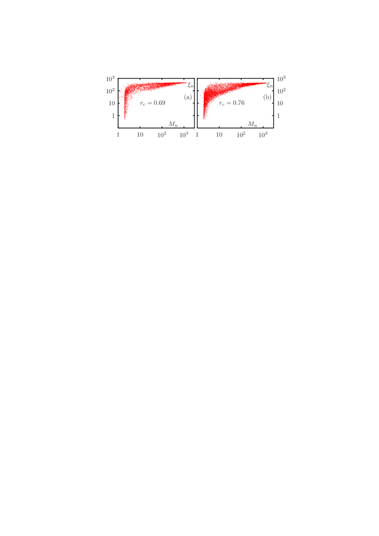
Figure 1: Gyration radii $\xi_{n}$ vs the the participation numbers $M_{n}$ of all modes with polarization perpendicular to the plane (a) and parallel to the plane (b). Parameters: $N=4000$, $L=1000D$ and $\lambda=100D$. Numerical value of the correlation coefficient $r_{c}$ between $M_{n}$ and $\xi_{n}$, calculated for all modes, is indicated in each plot.

The second approach to defining localization which has been used in the literature is based on the eigenmode radiative quality factor [11, 12] $Q_{n}$. Again, this definition rests on the analogy with bound states in quantum mechanics and the assumption of exponential localization. However, it is easy to see that propagating modes in three-dimensional transparent periodic or homogeneous media are all strictly non-radiating (with $\gamma_{n}=0$). An example of a propagating mode in a one-dimensional periodic chain which is strictly non-radiating, is given in Ref. [21]. On the other hand, radiating modes in an RPC can, in principle, be localized. This is illustrated in Fig. 2. Here we plot the inverse radiative quality factors $\gamma_{n}$ vs the corresponding values of $M_{n}$ for the same set of parameters as in Fig. 1. First, it can be seen that, while the localized modes tend to be of higher quality, the correlation is not very strong (numerical values of the correlation coefficient $r_{c}$ are indicated in each plot). Second, there are two visibly distinct “branches” in Fig. 2(a) (${\bf E}_{\rm inc}$ perpendicular to the RPC). The top, lower quality, branch corresponds to modes with non-vanishing dipole moments. According the criterion $M_{n}\ll N$, a significant number of such modes is localized.

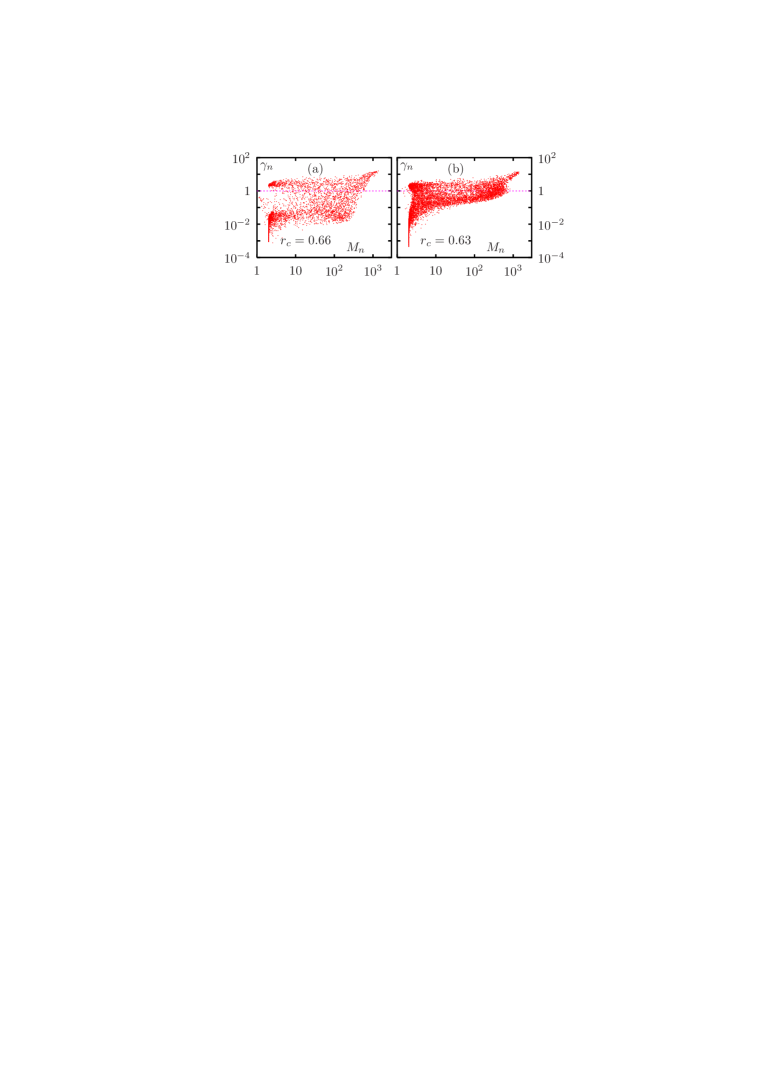
Figure 2: Inverse radiative quality factors $\gamma_{n}$ vs $M_{n}$. Same parameters as in Fig. 1. Numerical value of the correlation coefficient $r_{c}$ between $M_{n}$ and $\gamma_{n}$ is indicated in each plot.

6 Localization-Delocalization Transition

So far, we have seen that some of the modes are localized on just a few inclusions. Now we investigate if these modes actually form a band. To this end, we plot in Figs. 3 and 4 the values of $M_{n}$ vs the appropriate spectral parameter of the theory, which is the real part of the corresponding eigenvalue $w_{n}$. To see that ${\rm Re}w_{n}$ is, indeed, the spectral parameter analogous to energy, consider the following. The $n$-th mode is resonantly excited at an electromagnetic frequency $\omega$ such that ${\rm Re}[z(\omega)-w_{n}(\omega)]=0$ while for an isolated spherical inclusion the resonance condition is ${\rm Re}[z(\omega)]=0$. Thus, the real parts of the eigenvalues describe shifts of resonant frequencies of collective excitations relative to the respective value in the non-interacting limit. This can be illustrated with the following simple example. Let the polarizability of a single inclusion be given by the Lorenz-Lorentz formula with the first non-vanishing radiative correction [24], namely,

$$z=\frac{1}{\alpha}=\left(\frac{2}{D}\right)^{3}\frac{\epsilon+2\epsilon_{h}}{\epsilon-\epsilon_{h}}-i\frac{2k^{3}}{3}\ ,$$ (19)

where $\epsilon_{h}$ is the dielectric constant of the transparent host and $\epsilon$ is the dielectric constant of the inclusions. Further, let $\epsilon$ be given by the Drude’s formula

$$\epsilon(\omega)=\epsilon_{0}-\omega_{p}^{2}/\omega(\omega+i\Gamma)\ ,$$ (20)

where $\Gamma$ is the relaxation and $\epsilon_{0}$ is the intra-band input to the dielectric function. For simplicity, let us also assume that $\epsilon_{0}=\epsilon_{h}$ (this will not influence any conclusions in a significant way). Then the resonance condition for the $n$-th eigenmode takes the following form:

$$D^{3}{\rm Re}w_{n}=8\left(1-3\epsilon_{h}\omega^{2}/\omega_{p}^{2}\right)\ .$$ (21)

Optical resonance for an isolated spherical inclusion takes place at the Fröhlich frequency $\omega_{F}=\omega_{p}/\sqrt{3\epsilon_{h}}$. The corresponding resonance mode is characterized by ${\rm Re}w_{n}=0$. Electromagnetic interaction of the inclusions results in appearance of eigenmodes which are characterized by ${\rm Re}w_{n}\neq 0$. Corresponding spectral resonances take place at frequencies different from $\omega_{F}$. Using the above model for $z=1/\alpha$ and $\epsilon$, we can estimate that the spectral shifts shown in Figs. 3,4 are limited to $0.86\omega_{F}<\omega<1.12\omega_{F}$ which corresponds to $-2<D^{3}{\rm Re}w_{n}<2$. Note that much larger spectral shifts can be obtained for larger densities of inclusions. However, consideration of larger densities requires that calculations are carried out beyond the dipole approximation.

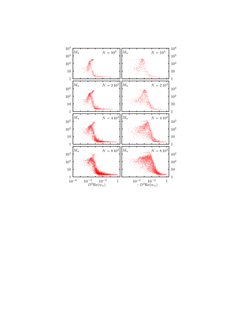
Figure 3: Participation numbers $M_{n}$ vs dimensionless spectral parameters $D^{3}{\rm Re}w_{n}$ for different densities of inclusions. Polarization is perpendicular to the RPC, other parameters same as in Figs. 1 and 2.

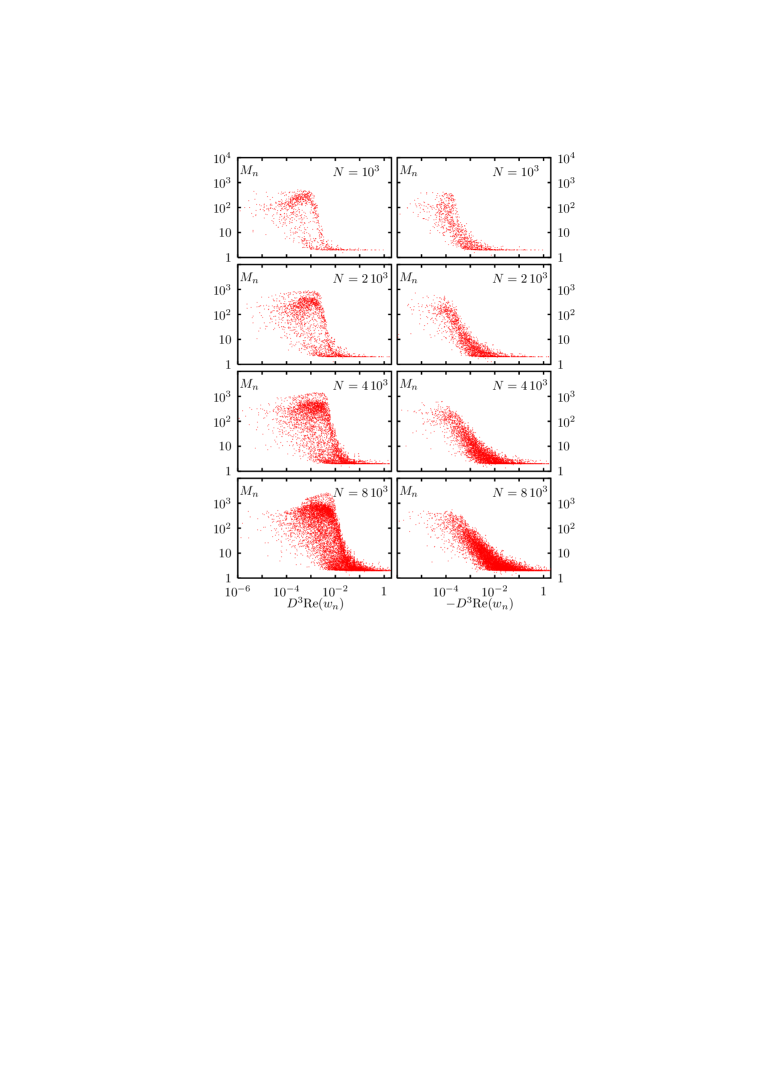
Figure 4: Same as in Fig 3 but for polarization being parallel to the RPC

Modes polarized perpendicular to the RPC are shown in Fig. 3. The data for parallel polarization are shown in Fig. 4. Analysis of Figs. 3,4 clearly reveals a transition from delocalized to localized states. In particular, all states with sufficiently large values of $D^{3}|{\rm Re}w_{n}|$ are localized. Such states are characterized by relatively strong interaction. In the case of low density ($N=10^{3}$, $\ell\approx 32D$), most of the localized states are binary, i.e., involve excitation of only two inclusions. As the density of inclusions increases, localized modes involving three, four and more inclusions emerge. For eigenmodes polarized perpendicular to the RPC plane and in the spectral region ${\rm Re}w_{n}>0$, there are also eigenstates with $M_{n}=1+p$, $p\ll 1$. It can be argued that such modes are localized on just one inclusion. Yet, ${\rm Re}w_{n}$ for such modes is significantly shifted from the non-interacting limit ${\rm Re}w_{n}=0$ This result may seem to be contradictory. Indeed, if the eigenmode amplitude is very small on all but just one inclusion, the latter may be seen as not interacting with its environment. The contradiction is resolved as follows. Consider a mode with eigenvalue $w$ which is localized on the $i$-th inclusion. The corresponding eigenvector $|\psi\rangle$ must then satisfy

$$w\langle i\sigma|\psi\rangle=\sum_{j\neq i}\sum_{\tau}\langle i\sigma|W|j\tau\rangle\langle j\tau|\psi\rangle\ .$$ (22)

Here $\sigma,\tau$ label the Cartesian components of vectors and the index $n$ that labels eigenmodes is omitted; we thus focus attention only on the selected eigenstate. The eigenmode is localized on the $i$-th inclusion if $m({\bf r}_{i})=1-p$ where $p\ll 1$. Therefore $m({\bf r}_{i})\sim 1$ and, since the weights satisfy the sum rule (16), we also have $m({\bf r}_{j})\sim p/N$ for $j\neq i$. We now recall that the weights are quadratic in eigenvector components. Consequently, $\langle j\tau|\psi\rangle\sim\sqrt{p/N}$ for $j\neq i$ while $\langle i\sigma|\psi\rangle\sim 1$. It then follows from (22) that

$$w\sim N\langle W\rangle\sqrt{p/N}=\langle W\rangle\sqrt{pN}\ ,$$ (23)

where $\langle W\rangle$ is the appropriate average of the interaction operator in the right-hand side of (22) and the above relation is accurate only to the order of magnitude. We thus see that, even if $p$ is arbitrarily small, the spectral shift may not be small in a sufficiently large sample (large $N$). This result is not specific to the RPC’s but is valid in two and three-dimensional disordered media as well. Of course, the value of $\langle W\rangle$ will depend on the dimensionality of the sample and on the density of inclusions. We note that $\langle W\rangle$ is the same as the factor $Q$ introduced by Berry and Percival within the mean-field approximation [25].

The phenomenon of spectrally shifted eigenstates which are localized on just one inclusion is explained by constructive interference and has no counterpart for electrons in disordered solids. This is because the analogy between the spectral parameter ${\rm Re}w_{n}$ and energy is not complete. Indeed, in the case of the classic Anderson model, an electronic state can be localized at an anomalously deep local potential. Such state is not influenced in any way by values of potentials at neighboring sites since the electron is exponentially localized inside the potential well. But the localization phenomenon discussed here is, essentially, collective and depends on the particular realization of the random sample as a whole. Likewise, the binary states seen in Figs. 3,4 are not necessarily binary states of two closely situated inclusions which interact with the rest of the sample very weakly (although such states are also possible; see Ref. [13] for properties of isolated dimer states). This is evident already from the data shown in Fig. 1. Here some of the binary states (with $M_{n}\approx 2$) are characterized by large gyration radii $\xi_{n}$ and, therefore, are not localized on two closely placed inclusions.

It can also be seen that there is a spectral region (which depends on the density of inclusions and on polarization of the eigenmodes) where localized and delocalized modes co-exists simultaneously. This spectral region is especially well pronounced in the case of larger densities and for polarization of eigenmodes parallel to the plane of the RPC. Co-existence of localized and delocalized modes with very close spectral parameters has been previously demonstrated for random three-dimensional fractal aggregates and was referred to as inhomogeneous localization [26]. Inhomogeneous localization was also observed in the case of RPCs [4]. However, the findings of Refs. [4, 26] were based on the quasistatic approximation and on the definition (17) of the localization length. It was concluded that localization is inhomogeneous in the whole spectral range. Here we show that inhomogeneous localization takes place only in a transitional energy band. The width of this transitional band as a function of system size and density of inclusions needs to be further investigated, especially, without the use of dipole approximation.

7 Coupling of Localized Models to the Far Field

We now consider the possibility of coupling of localized modes to the external field. It has been previously argued that, in the quasistatic limit, strongly localized modes can not be effectively coupled to plane waves. Therefore, such modes were referred to as dark [4]. However, the dark modes become coupled to external plane waves if one considers first non-vanishing corrections in $k$, i.e., goes beyond the quasistatic limit. For example, in Ref. [13] it was shown that the fully antisymmetrical mode of two oscillating dipoles (with zero total dipole moment) can be effectively coupled to an external plane wave in the limit $kL\rightarrow 0$. This coupling is explained by a small phase shift of the incident wave and the high quality factor of the mode. Indeed, it can be seen from (7) that under the exact resonance condition ${\rm Re}(z-w_{n})=0$, the excited dipole moments become proportional to $f_{n}^{\rm(eff)}=Q_{n}f_{n}$, where $Q_{n}=1/\gamma_{n}$. Thus, even in samples that are small compared to the wavelength, high-quality modes with zero or vanishing dipole moment can be effectively excited under the resonance condition. When the sample size is not small compared to the wavelength, even the strict resonance condition is not required for effective coupling. This is illustrated in Fig. 5. Here we plot the coupling constants $f_{n}$ vs $M_{n}$ for the same set of parameters as in Figs. 1 and 2. Since the coupling constants are normalized by the condition $\sum_{n}f_{n}=N$, a mode is coupled effectively if $f_{n}\sim 1$. The modes with $f_{n}\ll 1$ are coupled weakly and the modes with $f_{n}\sim N$ are coupled strongly. Correlation between $M_{n}$ and $f_{n}$ appears to be quite weak (see the figure for numerical values of the correlation coefficient $r_{c}$). Most importantly, it can be seen that a considerable fraction of localized modes is effectively coupled to the external wave, although only delocalized modes can be coupled strongly.

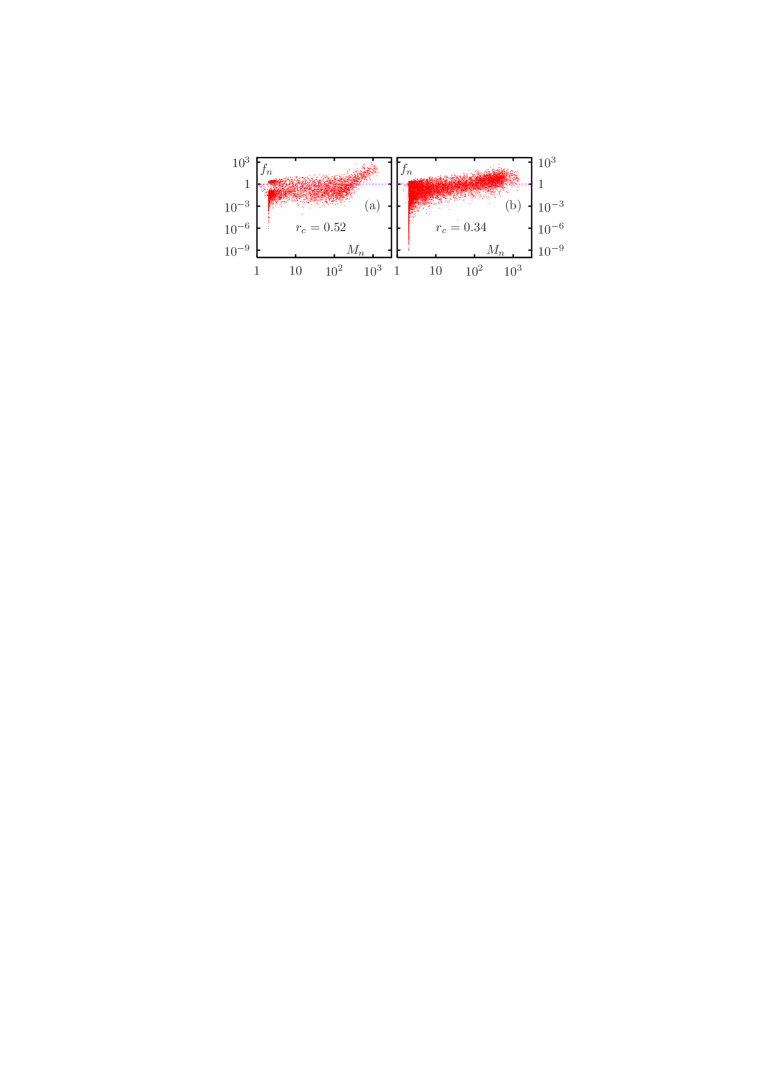
Figure 5: Coupling constants $f_{n}$ vs participation numbers $M_{n}$. Coupling constants are computed for an external plane wave ${\bf k}_{\rm inc}=k\hat{\bf x}$ and ${\bf E}_{\rm inc}=E_{0}\hat{\bf z}$ (a) and for ${\bf k}_{\rm inc}=k\hat{\bf z}$ and ${\bf E}_{\rm inc}=E_{0}(\hat{\bf x}+\hat{\bf y})/\sqrt{2}$ (b). Other parameters same as in Fig. 1. Numerical value of the correlation coefficient $r_{c}$ between $M_{n}$ and $f_{n}$ is indicated in each plot.

Perhaps, the most counter-intuitive fact about the polar eigenmodes that can be understood only beyond the quasistatics is that the inverse radiative quality factor $\gamma_{n}$ and the coupling constant $f_{n}$ are not necessarily proportional to each other. In Figs. 6,7 we plot $f_{n}$ vs $\gamma_{n}$ for different ratios $\lambda/L$ and for mode polarization perpendicular to the RPC (Fig. 6) and parallel to the RPC (Fig. 7). First, consider the case of orthogonal polarization. In the quasistatic limit, it can be shown [14] that (for this particular polarization of the eigenmodes) $f_{n}=\gamma_{n}$. This proportionality is clearly visible in the case $\lambda/L=12.8$ and the correlation coefficient $r_{c}$ between $\gamma_{n}$ and $f_{n}$ exceeds $0.999$. However, at smaller values of $\lambda/L$, there is no strict proportionality. Thus, for example, in the case $\lambda/L=0.02$, the correlation coefficient is rather small ($r_{c}=0.42$). It can also be seen that the modes with $\gamma_{n}\approx 1$ have coupling constants which differ by four orders of magnitude and can be either weakly or strongly coupled to the far field. Likewise, modes that are effectively coupled to the far field ($f_{n}\approx 1$) can be either weakly radiating ($\gamma_{n}\ll 1$) or strongly radiating ($\gamma_{n}\gg 1$).

Now consider eigenmodes which are polarized in the RPC plane (Fig. 7). There are two linearly-independent in-plane polarizations of the incident wave, ${\bf E}_{\rm inc}$. While the radiative factors are independent of ${\bf E}_{\rm inc}$, this is not so for $f_{n}$’s. For any given direction of ${\bf E}_{\rm inc}$, there is no strict proportionality between $\gamma_{n}$ and $f_{n}$ even in the quasistatic limit. This lack of proportionality is a consequence of polarization effects. For example, there might be modes which are strongly coupled to incident waves polarized along the $x$-axis but not coupled to waves polarized along the $y$-axis. However, the polarization effects can be suppressed by taking the average of $f_{n}$ over two linearly-independent incident polarizations. We denote such average as $\langle f_{n}\rangle$ and it can be shown that in the quasistatic limit $\langle f_{n}\rangle=\gamma_{n}/2$. This is indeed confirmed by the data shown in Fig. 7. Qualitatively, the data in Fig. 7 are similar to those shown in Fig. 6, with even smaller correlation factors.

The finding that weakly radiating modes can be effectively coupled to propagating waves is counter-intuitive and even may seem to contradict conservation of energy. Indeed, consider excitation of a mode which is effectively coupled to the far field but is weakly radiating by an electromagnetic wave that is “turned on” at an initial moment of time $t=0$. Since the mode is weakly radiating, it would not contribute significantly to the scattered field. Thus the incident wave would seemingly pass through the sample without noticeable scattering or absorption. However, at a sufficiently large time $t=T$, a steady state would be reached, in which a finite electromagnetic energy would be transferred to plasmonic oscillations in the mode. Since the incident wave was not scattered or absorbed, this contradicts energy conservation. In fact, the contradiction is resolved by noticing that a given mode is weekly radiating only at a fixed electromagnetic frequency $\omega$. (Beyond the quasistatic limit, both the eigenvectors $|\psi_{n}\rangle$ and the eigenvalues $w_{n}$ are functions of $\omega$.) But the transition process described above necessarily involves incident waves of different frequencies, not all of which would pass through the sample without scattering. This would result in non-zero extinction of the incident power.

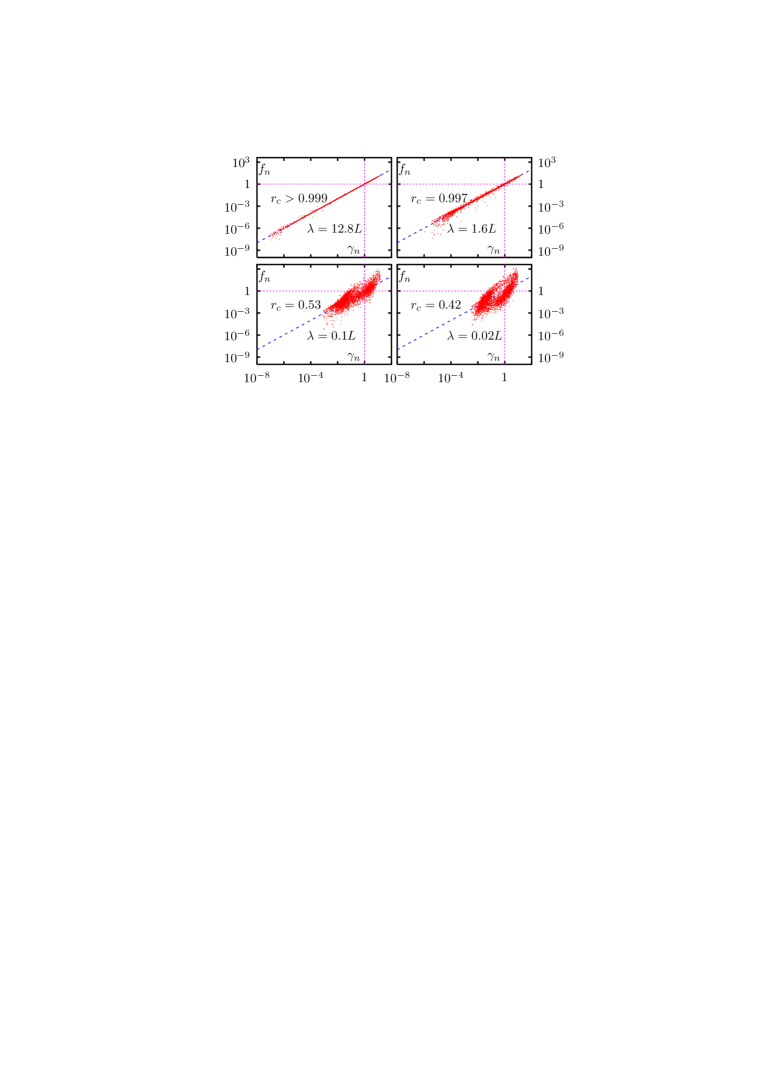
Figure 6: Coupling constants $f_{n}$ vs inverse radiative quality factors $\gamma_{n}$ for all modes polarized perpendicular to the RPC with $N=4000$ inclusions and different ratios $\lambda/L$, as indicated. In all cases, $L=1000D$. The dashed blue line corresponds to the quasistatic result $f_{n}=\gamma_{n}$. Numerical values of the correlation coefficient $r_{c}$ between $\gamma_{n}$ and $f_{n}$ are indicated.

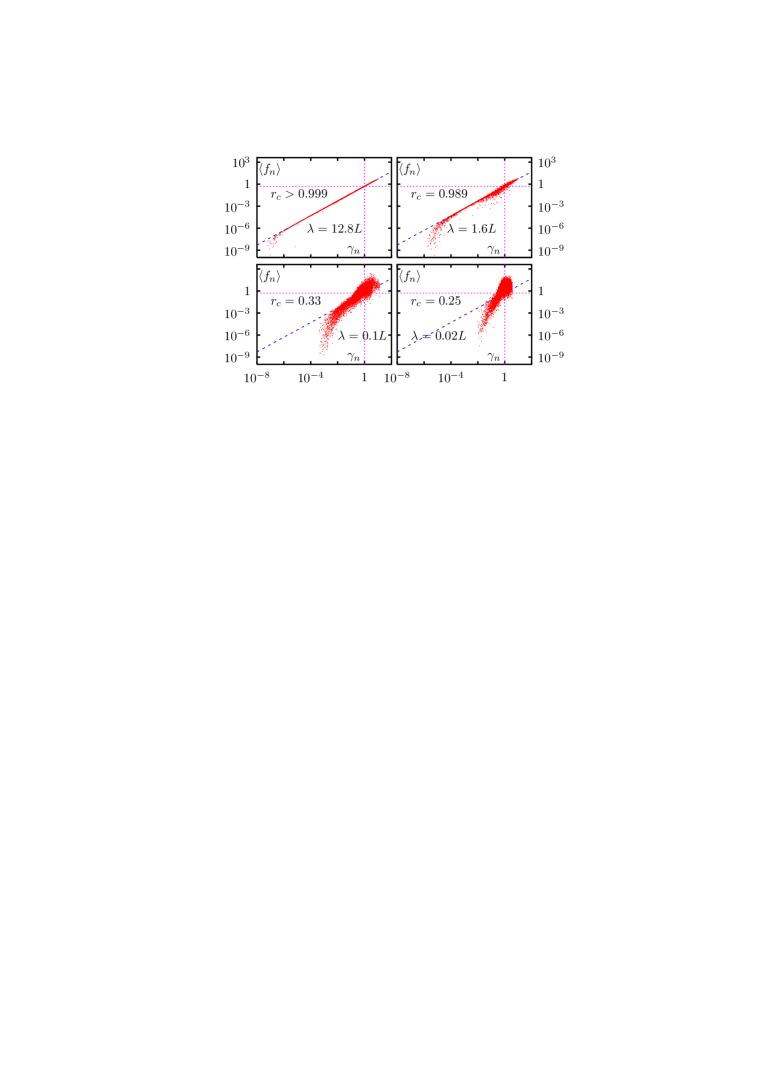
Figure 7: Same as in Fig. 6 but for modes polarized in plane of the RPC and the coupling coefficients $f_{n}$ are averaged over the two orthogonal in-plane polarizations of the incident wave. The dashed blue line corresponds to the quasistatic result $\langle f_{n}\rangle=\gamma_{n}/2$ and $\langle\ldots\rangle$ denotes polarization averaging. Numerical values of the correlation coefficient $r_{c}$ between $\gamma_{n}$ and $\langle f_{n}\rangle$ are indicated.

8 Summary and Discussion

Localization of polar eigenmodes in random planar composites (RPCs) has been studied theoretically and numerically without the quasistatic approximation. It was demonstrated that the localization criteria based on exponential confinement (analogy with electrons in solids) can not be applied to polar excitations in disordered composites and in RPCs in particular. This is because localization of polar eigenmodes is algebraic rather than exponential. Still, eigenstates with algebraically decaying tails can be square-integrable and discrete, and therefore, localized in the Anderson sense.

Note that localized eigenstates whose tails decay according to power law have been also discovered for Hamiltonians which can be represented by so-called random banded matrices with algebraically decaying bands [27]. Elements of such matrices $a_{ij}$ decay as $|i-j|^{-\alpha}$. Here $|i-j|$ can be viewed as a liner distance in a one-dimensional system. It was found that for $\alpha<1$ all eigenstates are delocalized while for $\alpha>1$ all eigenstates are algebraically localized. In the critical case $\alpha=1$, the structure of eigenstates was found to be multifractal. These findings were in agreement with the results obtained earlier for random mechanical oscillators coupled by quasistatic dipole-dipole interaction in Refs. [28, 29]. In these references, the long-range interaction was accounted for perturbatively, but arbitrary dimensionality of space $d$ was considered, with the conclusion that all eigenstates are delocalized when $\alpha\leq d$. We note that there are several important physical differences between the model considered here and in Refs. [28, 29, 27]. For example, in [29] two mechanical oscillators are in resonance irrespectively of the distance between them if their frequencies exactly coincide. In the model discussed here, resonances are not mechanical but electromagnetic, with resonance frequency strongly depending on the geometrical arrangement of dipoles . Instead of solving the problem of weakly coupled oscillators of random frequencies, we solve the problem of electromagnetically coupled, identical polarizable particles. Further, a random banded matrix of size $N$ has $N^{2}$ mathematically independent elements while the interaction operator $W$ of size $N$ (studied in this paper) depends on only $N$ mathematically independent variables ${\bf r}_{i}$ and is not banded. However, the mathematical reason for algebraic rather than exponential localization appears to be similar in both models: the algebraic spatial decay of interaction. Theory of localization for systems whose Hamiltonian can be represented by power-law band random matrices was further developed in Refs. [30, 31, 32, 33]. It is interesting to note that electromagnetic interaction in the radiation zone decays as $r^{-1}\exp(ikr)$ and $d=2$ for the RPCs. Thus, the rate of algebraic decay corresponds to the regime $\alpha<d$. However, the interaction is modulated by the exponential phase factor $\exp(ikr)$ which makes a direct comparison of results problematic.

Since localized states in an RPC have algebraically decaying tails, the previously used localization criterion based on the gyration radius of the mode is inapplicable. Consequently, an alternative approach based on the participation number has been used in this paper. It was shown that all electromagnetic states in the RPC whose resonance frequencies are shifted from those of non-interacting inclusions by a value larger than certain threshold are localized. The band of localized states shown in Figs. 3 and 4 for sufficiently large values of $|{\rm Re}(w_{n})|$ can be mapped to an interval of electromagnetic frequencies if the material properties of the inclusions and the host medium are specified. It should be noted that much stronger spectral shifts will be observed at higher concentrations of inclusions. Consideration of the high-density limit will require solving the electromagnetic problem without the dipole approximation. When applied to large random systems, this is a very computationally demanding procedure, solution to which, at least at the time being, appears to be not feasible. The author expects that this will not influence the localization properties of the eigenmodes.

Finally, possibility of coupling of localized modes to the far field has been studied. It was shown that, contrary to the previous belief, localized modes in the RPCs can be effectively coupled to the far field.

References

References

- [1] van Rossum M C W and Nieuwenhuizen T M 1999 Rev. Mod. Phys. 71(1) 313–371
- [2] Lee P A and Ramakrishnan T V 1985 Rev. Mod. Phys. 57(2) 287–337
- [3] Cao H 2005 J. Phys. A 38 10497–10535
- [4] Stockman M I, Faleev S V and Bergman D J 2001 Phys. Rev. Lett. 87(16) 167401
- [5] Drachev V P, Thoreson M D, Khaliullin E N, Davison V J and Shalaev V M 2004 J. Phys. Chem. B 108(46) 18046–18052
- [6] Drachev V P, Nashine V C, Thoreson M D, Ben-Amotz D, Davisson V J and Shalaev V M 2005 Langmuir 21(18) 8368–8373
- [7] Drachev V P, Thoreson M D, Nashine V, Khalliullin E N, Ben-Amotz D, Davisson V J and Shalaev V M 2005 J. Raman Spectr. 36 648–656
- [8] Carney P S and Schotland J C 2001 Opt. Lett. 26 1072–1074
- [9] Carney P S, Frazin R A, Bozhevolnyi S I, Volkov V S, Boltasseva A and Schotland J C 2004 Phys. Rev. Lett. 92 163903
- [10] Genov D A, Shalaev V M and Sarychev A K 2005 Phys. Rev. B 72 113102
- [11] Rusek M, Orlowski A and Mostowski J 1997 Phys. Rev. E 56(4) 4892
- [12] Rusek M, Mostowski J and Orlowski A 2000 Phys. Rev. A 61(2) 022704
- [13] Markel V A 1992 J. Mod. Opt. 39(4) 853–861
- [14] Markel V A 1995 J. Opt. Soc. Am. B 12(10) 1783–1791
- [15] Bergman D J 1978 Phys. Rep. 43 377
- [16] Rojas R and Claro F 1986 Phys. Rev. B 34(6) 3730–3736
- [17] Fuchs R and Claro F 1989 Phys. Rev. B 39(6) 3875–3878
- [18] Claro F and Fuchs R 1991 Phys. Rev. B 44(9) 4109–4116
- [19] Markel V A and Poliakov E Y 1997 Phil. Mag. B 76(6) 895–909
- [20] Markel V A and Sarychev A K 2006 Phys. Rev. B Submitted
- [21] Burin A L, Cao H, Schatz G C and Ratner M A 2004 J. Opt. Soc. Am. B 21(1) 121–131
- [22] Kramer B and MacKinnon A 1993 Rep. Prog. Phys. 56 1469–1564
- [23] Anderson P W 1978 Rev. Mod. Phys. 50(2) 191–201
- [24] Draine B T 1988 Astrophys. J. 333 848–872
- [25] Berry M V and Percival I C 1986 Optica Acta 33(5) 577–591
- [26] Stockman M I, Pandey L N and George T F 1996 Phys. Rev. B 53(5) 2183–2186
- [27] Mirlin A D, Fyodorov Y V, Dittes F M, Quezada J and Seligman T H 1996 Phys. Rev. E 54(4) 3221–3230
- [28] Levitov L S 1989 Europhys. Lett. 9(1) 83–86
- [29] Levitov L S 1990 Phys. Rev. Lett. 64(5) 547–550
- [30] Mirlin A D and Evers F 2000 Phys. Rev. B 62(12) 7920–7933
- [31] Varga I 2002 Phys. Rev. B 66 094201
- [32] Cuevas E, Ortuno M, Gasparian V and Perez-Garrido A 2002 Phys. Rev. Lett. 88(1) 016401
- [33] Cuevas E 2003 Phys. Rev. B 68 024206