Pulse Normalisation in Slow-Light Media

Abstract

We analytically study the linear propagation of arbitrarily shaped light-pulses through an absorbing medium with a narrow transparency-window or through a resonant amplifying medium. We point out that, under certain general conditions, the pulse acquires a nearly Gaussian shape, irrespective of its initial shape and of the spectral profile of the line. We explicitly derive in this case the pulse parameters, including its skewness responsible for a deviation of the delay of the pulse maximum from the group delay. We illustrate our general results by analysing the slow-light experiments having demonstrated the largest fractional pulse-delays.

I INTRODUCTION

The principle underlying most of the slow-light experiments is to exploit the steep normal dispersion of the refractive index associated with a pronounced peak in the transmission of the medium and the correlative reduction of the group velocity. The situation where the resulting time-delay of the light-pulse is large compared to its duration and can be controlled by an external laser field is of special importance for potential applications, especially in the domain of high-speed all-optical signal-processing. Harris and his co-workers ref1 ; ref2 opened the way to such experiments by exploiting the phenomenon of electromagnetically induced transparency (EIT) allowing one to create a narrow transparency-window in an otherwise optically thick atomic vapour. Using a true-shape detection of the pulses, they demonstrated propagation velocities as slow as $c/165$ and group delays $\tau_{g}$ as long as $4.6\>\tau_{in}$ where $c$ and $\tau_{in}$ are respectively the velocity of the light in vacuum and the full width at half-maximum (FWHM) of the intensity-profile of the incident pulse. Much slower velocities have been attained in subsequent EIT experiments (for reviews see, e.g., ref3 ; ref4 ; ref5 ) and in experiments involving coherent population oscillations ref6 or other processes to induce a transparency-window in an absorbing medium. It is however worth noticing that only few of these experiments, all using EIT, have succeeded in giving direct demonstrations of fractional delays $\tau_{g}/\tau_{in}$ exceeding unity ref2 ; ref7 ; ref8 . Theoretical discussions on the maximum time-delays attainable in such experiments can be found in ref1 ; ref9 ; ref10 . A different way to achieve a system with a controllable transmission-peak is to optically induce a resonant gain in a transparent medium ref11 . Initially proposed by Gauthier ref12 , the arrangement involving stimulated Brillouin scattering ref13 ; ref14 ; ref15 ; ref16 seems particularly attractive from the viewpoint of the above mentioned applications. The Brillouin gain is indeed directly implemented on an optical fibre and there are no severe constraints in the choice of the operating wavelength. The group delay $\tau_{g}$ has already been controlled on a range of $3.6\>\tau_{in}$ by this technique ref15 . Note that preliminary experiments using a Raman fibre amplifier have also been achieved ref17 .

The purpose of our paper is to provide analytical results on the propagation of arbitrarily shaped pulses, the central frequency of which coincides with that of a pronounced maximum in the medium-transmission. We examine more specifically the case where the resulting time-delays of the pulses are large compared to their duration. Our study applies in particular but not exclusively to the above mentioned systems. Our approach follows in part and extends that of Bukhman ref18 with a special attention paid to the connection of the theoretical results with the experiments.

II GENERAL ANALYSIS

We denote by $e_{in}(t)$ and $e_{out}(t)$ the slowly-varying envelopes of the incident and transmitted pulses and by $E_{in}(\Omega)=\int_{-\infty}^{\infty}e_{in}(t)\exp(-i\Omega t)dt$ and $E_{out}(\Omega)$ their Fourier transforms. The slow-light medium is characterised by its impulse response $h(t)$ or by its transfer function $H(\Omega)$, Fourier transform of $h(t)$. The input/output relation or transfer equation reads $e_{out}(t)=h(t)\otimes e_{in}(t)$ in the time-domain or $E_{out}(\Omega)=H(\Omega)E_{in}(\Omega)$ in the frequency-domain ref19 . We assume that the incident pulse has a finite energy, that it is not chirped ($e_{in}(t)$ real and positive) and that $h(t)$ is also real. The local response of the medium is characterised by the complex gain-factor $\Gamma(\Omega)=\ln\left[H(\Omega)\right]$ whose real part $F(\Omega)$ and imaginary part $\Phi(\Omega)$ are respectively the logarithm of the medium amplitude-gain $\left|H(\Omega)\right|$ and the induced phase shift. The condition imposed to $h(t)$ implies that $H(-\Omega)=H^{*}(\Omega)$ and thus that $F(\Omega)$ and $\Phi(\Omega)$ are respectively even and odd functions of $\Omega$. This has the advantage of eliminating the lowest-order pulse-distortions resulting from the gain-slope and from the group velocity dispersion at the frequency $\omega_{0}$ of the optical carrier ($\Omega=0$). Moreover the medium is then entirely characterised by the single real function $h(t)$. In order to have simple expressions we use for $e_{in}(t)$ a time origin located at the pulse centre-of-gravity and for $e_{out}(t)$ a time origin retarded by the transit time at the group velocity outside the frequency-domain of high-dispersion (local time picture). The time delays considered hereafter are thus only those originating in the high-dispersion region.

General properties of the transmitted pulse can be derived by Fourier analysis. Let $x(t)$ be any of the real functions $e_{in}(t)$, $h(t)$ or $e_{out}(t)$ and $X(\Omega)$ its Fourier transform. We remark that $X(0)=\int_{-\infty}^{\infty}x(t)dt$ and, following an usual procedure in probability theory ref20 , we characterise $X(\Omega)$ by its cumulants $\kappa_{n}$, such that

$$X(\Omega)=X(0)\exp\left(\sum_{n=1}^{\infty}\frac{\kappa_{n}}{n!}(-i\Omega)^{n}\right).$$ (1)

For $H(\Omega)$, we see that the cumulants are simply related to the coefficients of the series expansion of $\Gamma(\Omega)$ in powers of $-i\Omega$ and, in particular, that $\kappa_{1}$ coincides with the group delay $\tau_{g}=-\frac{d\Phi}{d\Omega}\mid_{\Omega=0}$. We incidentally recall that, due to the causality principle, $\tau_{g}$ can be related to the gain profile ref21 ; ref22 . Within our assumptions, this relation reads

$$\tau_{g}=P\int_{-\infty}^{\infty}\frac{\ln H_{0}-\ln\left|H(\Omega)\right|}{\pi\Omega^{2}}d\Omega$$ (2)

where $H_{0}=H(0)$ is the amplitude-gain of the medium at the frequency of the optical carrier. This confirms that large group delays are achieved when the gain $\left|H(\Omega)\right|$ has a pronounced maximum at $\Omega=0$. We have then $\kappa_{2}>0$.

Coming back to the general problem, we characterise the time function $x(t)$ by its area $S=\int_{-\infty}^{\infty}x(t)dt$ and its three lowest order moments, namely the mean value $\left\langle t\right\rangle=\frac{1}{S}\int_{-\infty}^{\infty}t\>x(t)dt$, the variance $\sigma^{2}=\frac{1}{S}\int_{-\infty}^{\infty}(t-\left\langle t\right\rangle)^{2}x(t)dt$ and the $3^{rd}$ order centred moment $a=\frac{1}{S}\int_{-\infty}^{\infty}(t-\left\langle t\right\rangle)^{3}x(t)dt$ . We recognise in $\left\langle t\right\rangle$ (resp. $\sigma$) the location of the centre-of-gravity (resp. the rms duration) of the function $x(t$). Its asymmetry may be characterised by the dimensionless parameter $\xi=a/\sigma^{3}$, the so-called skewness ref20 . For a Gaussian function, $\sigma=\tau/(2\sqrt{\ln 2})$ where $\tau$ is the FWHM of the energy profile $x^{2}(t)$. An important result ref20 is that the moments $\left\langle t\right\rangle$ , $\sigma^{2}$ and $a$ of $x(t)$ are equal to the cumulants $\kappa_{1},\kappa_{2}$ and $\kappa_{3}$ of $X(\Omega)$. Moreover the transfer equation immediately leads to the relations $E_{out}(0)=H_{0}E_{in}(0)$ and $\kappa_{n,out}=\kappa_{n,in}+\kappa_{n}$ where, as in all our paper, the indexes $in$, $out$ and the absence of index respectively refer to the incident pulse, the transmitted pulse and the transfer-function or impulse response of the medium. With our choice of time origin, $\left\langle t_{in}\right\rangle=0$. By combining the previous results, we finally obtain the four equations $S_{out}=H_{0}S_{in}$, $\left\langle t_{out}\right\rangle=\tau_{g}$, $\sigma_{out}^{2}=\sigma_{in}^{2}+\sigma^{2}>\sigma_{in}^{2}$ and $a_{out}=a_{in}+a$. In the studies of the linear pulse propagation, the first equation which relates the areas of the transmitted and incident pulses is known as the area theorem ref23 . The second equation expresses that the time-delay of the pulse centre-of-gravity equals the group delay ref22 . The two last ones specify how the rms duration and the asymmetry of the incident pulse are modified by the medium. All these results are valid provided that the involved moments are finite ref19 .

III ANALYTIC EXPRESSIONS OF THE MEDIUM IMPULSE-RESPONSE

In order to obtain a complete information on the shape and the amplitude of the transmitted pulse, we obviously have to specify the complex gain-factor $\Gamma(\Omega)$ of the medium. For the medium with a resonant gain, it reads

$$\Gamma(\Omega)=p_{N}(\Omega)G/2-A/2$$ (3)

where $p_{N}(\Omega)$ is the normalised complex profile of the gain-line ($p_{N}(0)=1$), $G$ is the gain parameter for the intensity ref14 and $A$ stands for the attenuation introduced to reduce the effects of the amplified spontaneous emission ref15 and/or to normalise the overall gain of the system. $G=g_{0}L$ where $g_{0}$(resp.$L$) is the resonance gain-coefficient (resp. the thickness) of the medium. The previous expression of $\Gamma(\Omega)$ also holds for an absorbing medium with a transparency-window when the absorption background is assumed to be infinitely wide. We then get $\Gamma(\Omega)=-[1-f\>p_{N}(\Omega)]\alpha_{0}L/2$ where $\alpha_{0}$ is the background absorption-coefficient, $f\leq 1$ specifies the depth of the transparency-window ref9 and $p_{N}(\Omega)$ is the normalised complex profile of the line associated with the transparency-window. By putting $G=f\>\alpha_{0}L$ and $A=\alpha_{0}L$ , we actually retrieve the expression of $\Gamma(\Omega)$ obtained for a gain medium. In both types of experiments, $G$ and $A$ are generally comparable in order that the resonance gain $H_{0}=\textrm{e}^{G/2-A/2}$ is close to 1 or, at least, does not differ too strongly from 1. Anyway the intensity-transmission on resonance exceeds its value far from resonance by the factor $\textrm{e}^{G}$.

To go beyond, it seems necessary to explicit the profile $p_{N}(\Omega)$. We first consider the reference case where $p_{N}(\Omega)$ is associated with a Lorentzian line. It then reads $p_{N}(\Omega)=1/(1+i\Omega/\gamma)$ where $\gamma$ is the half-width of the line ref22 and we immediately get $\kappa_{n}=Gn!/(2\gamma^{n})$ with in particular $\kappa_{1}=\tau_{g}=G/(2\gamma)$, $\kappa_{2}=\sigma^{2}=G/\gamma^{2}$ and thus $\tau_{g}=\sigma\sqrt{G}/2$. The last relation shows that achieving substantial fractional delays $\tau_{g}/\sigma$ requires that $G\gg 1$. A quite remarkable property of the Lorentzian case is that the impulse response has an exact analytical expression. This result has been obtained by Crisp in a general study on the propagation of small-area pulses in absorbing and amplifying media ref23 but it can easily be retrieved from $H(\Omega)$ by using standard procedures of Laplace transforms ref20 . One get

$$h(t)=\textrm{e}^{-A/2}\delta(t)+\textrm{e}^{-A/2}\gamma G\>\frac{I_{1}(\sqrt{2G\gamma t})}{\sqrt{2G\gamma t}}\>\textrm{e}^{-\gamma t}U(t)$$ (4)

where $\delta(t)$, $I_{1}(u)$ and $U(t)$ respectively designate the Dirac function, the $1^{st}$ order modified Bessel function and the unit step function. The $1^{st}$ term $h_{i}(t)$ in $h(t)$ results from the constant value $\textrm{e}^{-A/2}$ of $H(\Omega)$ far from resonance. This part of the response is instantaneous in our local time picture and only the $2^{nd}$ term $h_{d}(t)$, directly associated with the transmission peak, contribute to the delay. The areas of $h_{i}(t)$ and $h_{d}(t)$ are respectively $\textrm{e}^{-A/2}$ and $H_{0}-\textrm{e}^{-A/2}$, that is in a very small ratio ($\approx\textrm{e}^{-G/2}$ ) for the large values of $G$ required to achieve substantial delays (see above).

Figure 1: Analytical form of the impulse response for a Lorentzian line. From the left to the right the gain parameter $G$ (resp. the fractional delay $\tau_{g}/\sigma$) is 4, 9, 16, 25, 36, 49 and 64 (resp. 1, 1.5, 2, 2.5, 3, 3.5 and 4). The horizontal (resp. vertical) unit is $\sigma$ (resp. $H_{0}/\sigma\sqrt{2\pi}$ ).

The effect of the instantaneous response then becomes negligible. Fig.1 shows the delayed response obtained for increasing values of the gain and thus of the fractional group-delay. We see that the curves, first strongly asymmetric, become more and more symmetric as $G$ increases and that the location of their maximum then approaches the group delay. They have a discontinuity $H_{0}e^{-G/2}\gamma G/2$ at $t=0$, the relative amplitude of which becomes negligible when $G\gg 1$. From the asymptotic behaviour of $I_{1}(u)$ ref20 , we then get

$$h_{d}(t)\approx\frac{H_{0}}{\sigma\sqrt{2\pi}}\left(1-\frac{3\theta}{4\tau_{g}}\right)\exp\left(-\frac{\theta^{2}}{2\sigma^{2}}\right)$$ (5)

with $\theta=t-\tau_{g}$. The maximum of $h_{d}(t)$ occurs at the instant $\tau_{g}-\Delta t$ with $\Delta t\approx 3\sigma^{2}/(4\tau_{g})$. When $G\rightarrow\infty$,

$$h(t)\rightarrow h^{(2)}(t)=\frac{H_{0}}{\sigma\sqrt{2\pi}}\exp\left(-\frac{\theta^{2}}{2\sigma^{2}}\right).$$ (6)

This Gaussian form is that of the normal distribution derived by means of the central limit theorem in probability theory. This theorem can also be used for an approximate evaluation of the convolution of $n$ deterministic functions ref19 . It applies to our case by splitting the medium in $n$ cascaded sections, $h(t)$ being then the convolution of the impulse responses of each section. According to this analysis, one may expect that the normal form $h^{(2)}(t)$ is universal. From the frequency viewpoint, it originates in the fact that, when $G\gg 1$ , the transmission peak is roughly $\sqrt{G}$ times narrower than the line. In the region where the relative gain $\left|H(\Omega)\right|/H_{0}$ is not negligible, the curves $\Phi(\Omega)$ vs $\Omega$ (phase-shift) and $F(\Omega)$ vs $\Omega$ (line-profile) are well approximated respectively by a straight line and a parabola (Fig.2).

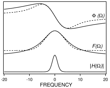
Figure 2: $\Phi(\Omega)$ and $F(\Omega)$ associated with a Lorentzian line (full line) and a Gaussian line (dashed line). The physical parameters are chosen in order that $H_{0}=0.6$ and $\tau_{g}/\sigma=3$ in both cases. The resulting gain profiles $\lvert H(\Omega)\rvert$ are indistinguishable at the figure scale. The frequency unit is $1/\sigma$ (angular frequency).

This means that only the first two cumulants $\kappa_{1}=\tau_{g}$ and $\kappa_{2}=\sigma^{2}$ play a significant role. We then get $H(\Omega)\approx H^{(2)}(\Omega)=H_{0}\exp(-i\Omega\tau_{g}-\sigma^{2}\Omega^{2}/2)$ and thus $h(t)\approx h^{(2)}(t)$ irrespective of the line-profile. This confirms the universality of the normal form of $h(t)$ when $G\rightarrow\infty$. In fact, $h^{(2)}(t)$ is a good approximation of the exact impulse-response for the gains currently achieved in the experiments. Fig.3 shows the result obtained with Lorentzian and Gaussian line-profiles when $\tau_{g}=3\sigma$. In the second case, $p_{N}(\Omega)=\exp(-\Omega^{2}/\gamma^{2})-2iD(\Omega/\gamma)/\sqrt{\pi}$ with $D(u)=\textrm{e}^{-u^{2}}\int_{0}^{u}\textrm{e}^{v^{2}}dv$ ref24 and the first cumulants read $\kappa_{1}=G/(\gamma\sqrt{\pi})$, $\kappa_{2}=G/\gamma^{2}$ and $\kappa_{3}=4G/(\gamma^{3}\sqrt{\pi})$. The parameters A, G and $\gamma$ are chosen such that $H_{0}$, $\tau_{g}$ and $\sigma$ have the same values in both cases. Though the line-profiles are quite different (see Fig.2), the impulse responses are both close to the normal form $h^{(2)}(t)$. Similar results (not shown) are obtained with other line-profiles, including the EIT profile (see hereafter).

When the gain parameter is large but not very large, a better approximation of the impulse response is obtained by considering the effect of the $3^{rd}$ cumulant $\kappa_{3}$, equal to the asymmetry parameter $a$ of $h(t)$. Provided that this effect may be considered as a small perturbation, $H(\Omega)\approx H^{(3)}(\Omega)\approx\left(1+i\kappa_{3}\Omega^{3}/3!\right)H^{(2)}(\Omega)$. From the correspondence $i\Omega\leftrightarrow d/dt$, we finally get

$$h(t)\approx h^{(3)}(t)\approx\left(1-\frac{a\theta}{2\sigma^{4}}\right)h^{(2)}(t).$$ (7)

This result generalises that obtained in the Lorentzian case where $a=3G/\gamma^{3}$ and $a/(2\sigma^{4})=3/(4\tau_{g})$. In the Gaussian case, we find $a/(2\sigma^{4})=2/(\pi\tau_{g})$, a value not far from the previous one. This explains why the two impulse responses are very close (see Fig.3). Anyway they are very well approximated by $h^{(3)}(t)$ in each case. Quite generally the maximum of $h^{(3)}(t)$ occurs at $\tau_{g}-\Delta t$ with $\Delta t\approx a/(2\sigma^{2})=\xi\sigma/2$ where $\xi$ is the skewness of $h(t)$. In all the above calculations we have implicitly assumed that $\Delta t$ is small compared to $\sigma$. This implies that $\left|\xi\right|\ll 2$ but we checked that $h^{(3)}(t)$ keeps a fairly good approximation of $h(t)$ for skewness up to $1$.

Figure 3: Comparison of the exact impulse-responses for the Lorentzian profile (full line) and the Gaussian profile (dashed line) to the normal form $h^{(2)}(t)$ (dotted line). The fit by the improved forms $h^{(3)}(t)$ (not shown for clarity) is nearly perfect. Parameters as in Fig.2. Units as in Fig.1.

IV NORMAL FORM OF THE TRANSMITTED PULSE

The impulse response being known, the envelope of the transmitted pulse is given by the relation $e_{out}(t)=h(t)\otimes e_{in}(t)$ and will generally differ from that of the incident pulse. However the distortion will be negligible if the duration of $h(t)$ is small compared to that of the pulse. We then get $h(t)\approx\delta(t-\tau_{g})\int_{-\infty}^{+\infty}h(t)dt$ and thus $e_{out}(t)\approx H_{0}\>e_{in}(t-\tau_{g})$. Since we are interested in the situations where the time delay is large compared to the pulse duration, we obtain the double condition $\sigma\ll\sigma_{in}\ll\tau_{g}$ which can only be met with extremely large gain parameters. Taking for example $\sigma=\sigma_{in}/7$ and $\tau_{g}=7\sigma_{in}$ that is $\tau_{g}=49\sigma$, we get $G\approx 9600$ in the Lorentzian case. Fig.4 shows the results obtained with these parameters. As expected the pulse distortion is small, even in the sensitive case of a square-shaped pulse. Note that the gain parameter considered is not unrealistic. It is comparable to that used by Harris and co-workers in their pioneering EIT experiment where $G\approx A\approx 6000$ ref2 .

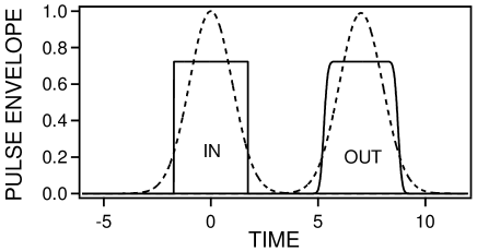
Figure 4: Propagation of a square-shaped (full line) and a Gaussian-shaped (dashed line) light-pulse with large delay and low distortion. The parameters are chosen in order that $\sigma=\sigma_{in}/7$, $\tau_{g}=7\sigma_{in}$ and $H_{0}=1$. The envelopes of the input pulses are given for reference. The time unit is the common rms duration $\sigma_{in}$ of the two incident pulses. As expected, the distortion of the Gaussian-shaped pulse is negligible and there is only a slight softening of the rise and of the fall of the square-shaped pulse.

However most of the direct demonstrations of large fractional pulse delays have been achieved with smaller gain parameters, typically ranging from 10 to 100, and with incident pulses whose rms duration $\sigma_{in}$ is comparable to and often smaller than $\sigma$. Substantial pulse-reshaping is then expected. Suppose first that the normal form $h^{(2)}(t)$ provides a good approximation of the impulse response and that the incident pulse is Gaussian-shaped. We have then $e_{in}(t)=\exp(-t^{2}/2\sigma^{2})$ and $e_{out}(t)$, convolution of two Gaussian functions, is itself Gaussian. It reads $e_{out}(t)=H_{0}(\sigma_{in}/\sigma_{out})\exp(-\theta^{2}/2\sigma_{out}^{2})$, where $\sigma_{out}^{2}=\sigma_{in}^{2}+\sigma^{2}$ . The effect of the medium on the light-pulse is simply to delay its maximum exactly by the group delay, to broaden it by the factor $\sqrt{1+\sigma^{2}/\sigma_{in}^{2}}$ [1, 9] and to modify its amplitude accordingly in order to respect the area theorem ref23 . Since this point is often overlooked, we stress that the broadening mechanism radically differs from that occurring in standard optical fibres ref25 . It originates in the $2^{nd}$ order gain-dispersion instead of in the group-velocity dispersion and the pulse envelope keeps real (no phase modulation or frequency chirping). In fact, provided that $\sigma_{in}$ be smaller than or comparable to $\sigma$ and that $\left|\xi_{in}\right|<1$, $e_{out}(t)$ is well approximated by a Gaussian function whatever the shape of the incident pulse is. This is again a consequence of the central limit theorem, the response $e_{out}(t)$ being obtained by an extra convolution added to those used to build $h(t)$. The conditions on $\sigma_{in}$ and $\left|\xi_{in}\right|$ originate in the requirement that all the terms to convolute should have moments of the same order of magnitude. We then obtain $e_{out}(t)\approx e_{out}^{(2)}(t)$ where $e_{out}^{(2)}(t)$ has the normal (Gaussian) form

$$e_{out}^{(2)}(t)=H_{0}\frac{S_{in}}{\sigma_{out}\sqrt{2\pi}}\exp\left(-\frac{\theta^{2}}{2\sigma_{out}^{2}}\right).$$ (8)

This result extends the previous one and shows that incident pulses having different shapes but the same area $S_{in}$ and the same variance $\sigma_{in}$ are reshaped in the medium to give approximately the same Gaussian-shaped pulse (Fig.5). From an experimental viewpoint, the dramatic reshaping of a square-shaped pulse has been clearly demonstrated (but not commented on) by Turukhin et al. ref8 in their EIT experiment in a solid (see their figure 2c for 0 probe detuning). Pulse reshaping is also apparent in the Brillouin scattering experiment by Song et al. ref13 where a flat-topped pulse is actually transformed in a gaussian-like pulse (see their figure 4 and compare the shapes obtained for gains 0dB and 30dB).

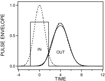
Figure 5: Example of pulse reshaping and broadening. The square-shaped (full line) and Gaussian-shaped (dashed line) incident pulses originate nearly identical transmitted pulses, respectively close and very close to the normal form $e_{out}^{(2)}(t)$ (dotted line). The time unit is $\sigma_{in}$ and the parameters are such that $\sigma=\sigma_{in}$, $\tau_{g}/\sigma=4$ and $H_{0}=1$. With this choice of $H_{0}$ and $\sigma$, the transmitted pulses have the same area that the incident ones (area theorem) and a rms duration $\sqrt{2}$ times larger.

A more precise approximation $e_{out}^{(3)}(t)$ of $e_{out}(t)$ can be obtained by taking into account the effect of the $3^{rd}$ order cumulants. Using the approach already used to determine $h^{(3)}(t)$, we get

$$e_{out}^{(3)}(t)\approx\left(1-\frac{a_{out}\theta}{2\sigma_{out}^{4}}\right)e_{out}^{(2)}(t)$$ (9)

with $a_{out}=a_{in}+a$. When the incident pulse is symmetric ($a_{in}=0$ ) as in most experiments, the skewness $\xi_{out}$ of the transmitted pulse reads $\xi_{out}=a/\left(\sigma^{2}+\sigma_{in}^{2}\right)^{3/2}$ and the pulse maximum occurs at $\tau_{g}-\Delta t_{out}$ with $\Delta t_{out}=a/\left[2\left(\sigma^{2}+\sigma_{in}^{2}\right)\right]$. Since $\left|\xi_{out}\right|<\left|\xi\right|$, the transmitted pulse is closer to a normal form than the impulse response of the medium. The previous results hold without restriction to the value of $\sigma_{in}$ when $e_{in}(t)$ is Gaussian. In the case of a Lorentzian line-profile, we easily get

$$\Delta t_{out}=\frac{3}{2\gamma\left(1+\sigma_{in}^{2}\gamma^{2}/G\right)}.$$ (10)

We have compared the theoretical delay of the pulse maximum, namely $\tau_{g}-\Delta t_{out}$, with the delay actually observed by Okawachi et al. in their Brillouin scattering experiment ref14 . Fig.6 shows this delay as a function of the gain parameter $G$ for two values of the pulse duration, respectively $\tau_{in}=63\>ns$ ($\sigma_{in}\approx 38\>ns$) and $\tau_{in}=15\>ns$ ($\sigma_{in}\approx 9\>ns$ ), with $\gamma=0.22\>ns^{-1}$ ($\gamma$ is the half of the full Brillouin linewidth $\Gamma_{B}$). Without any adjustment of parameters, our analytical results satisfactorily fit the observations. Note that the shifts $\Delta t_{out}$ are negligible for the longer pulse but significant for the shorter one.

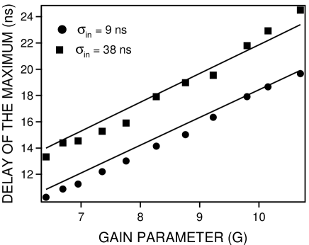
Figure 6: Comparison of the delays of the maximum of the transmitted pulse observed in a Brillouin scattering experiment ref14 (filled squares and circles) with our analytical predictions (full lines).

V EFFECT OF THE TRANSMISSION BACKGROUND

In the previous calculations, we have not taken into account the effect of the instantaneous part $h_{i}(t)=\textrm{e}^{-A/2}\delta(t)$ of the impulse response, arguing that its area is small compared to that of the delayed part. As a matter of fact, $h_{i}(t)$ originates a contribution $\textrm{e}^{-A/2}e_{in}(t)$ to $e_{out}(t)$, the amplitude of which is roughly $\textrm{e}^{G/2}\sigma_{in}/\sigma_{out}$ times smaller than that of the main part and is thus actually negligible in every case of substantial delay ($G\gg 1$, $\sigma_{out}$ and $\sigma_{in}$ of the same order of magnitude). We should however remark that this result lies on the assumption that the transmission peak is put on an uniform background.

We will now examine the case where the transmission background is not uniform. This happens in all the experiments where a transparency-window is induced in a absorption-profile of finite width, in particular in the EIT experiments. As an illustrative example we consider the simplest $\Lambda$ arrangement with a resonant control field. From the results given in ref4 , we easily get

$$\Gamma(\Omega)=-\frac{\gamma_{ba}\left(i\Omega+\gamma_{ca}\right)A/2}{\left(i\Omega+\gamma_{ba}\right)\left(i\Omega+\gamma_{ca}\right)+\Omega_{s}^{2}/4}$$ (11)

where $\gamma_{ba}$ (resp. $\gamma_{ca}\ll\gamma_{ba}$) is the coherence relaxation-rate for the probe transition (resp. for the forbidden transition), $\Omega_{s}$ is the modulus of the Rabi frequency associated with the control field and $A=\alpha_{0}L\gg 1$ is the resonance optical thickness in the absence of control field. The control field makes the resonance gain rise from $\textrm{e}^{-A/2}\approx 0$ to $H_{0}=\exp\left(-A\gamma_{ba}\gamma_{ca}/\left[2\left(\gamma_{ba}\gamma_{ca}+\Omega_{s}^{2}/4\right)\right]\right)$ and a good transparency is induced when $\Omega_{s}$ is larger than or comparable to $\gamma_{ba}\gamma_{ca}A$. The width of the transparency-window ($\propto$ $\Omega_{s}$/$\sqrt{A}$ ) is then much smaller than that of the absorption background ($\propto\gamma_{ba}\sqrt{A}$).

Without any approximation, the partial fraction decomposition of $\Gamma(\Omega)$ allows us to write the transfer-function of the medium as a product of simpler functions, namely $H(\Omega)=H_{1}(\Omega)H_{2}(\Omega)$ with $H_{j}(\Omega)=\exp\left[C_{j}/\left(i\Omega+\gamma_{j}\right)\right]$. According to the control power, the parameters $C_{1}$, $C_{2}$, $\gamma_{1}$ and $\gamma_{2}$ are real or complex. When $\Omega_{s}<(\gamma_{ba}-\gamma_{ca})$, $\gamma_{1}$ and $\gamma_{2}$ are real and positive whereas $C_{1}$ and $C_{2}$ are also real but of opposite sign. The EIT medium is then equivalent to a medium with two Lorentzian lines both centred at $\Omega=0$, respectively an absorption-line and a narrower gain-line. It is also equivalent to a cascade of a gain medium and an absorbing medium. When $\Omega_{s}>(\gamma_{ba}-\gamma_{ca})$, all the parameters are complex with $\gamma_{2}=\gamma_{1}^{*}$ and $C_{2}=C_{1}^{*}$ . The two lines are now located at $\Omega=\pm\textrm{Im}(\gamma_{1})$. They have the same intensity and the same width, but they are hybrid in the sense that, due to the complex nature of $C_{1}$ and $C_{2}$, their absorption and dispersion profiles are both the sum of an absorption-like and a dispersion-like profile. We incidentally note that the parameters used to obtain the figure 8 in ref4 correspond to such a situation. In all cases, the impulse responses associated to $H_{1}(\Omega)$ and $H_{2}(\Omega)$ have analytical expressions ref23 ; ref26 and the impulse response $h(t)$ of the medium is their convolution product. This general analysis is satisfactory from a formal viewpoint. It provides some physical insight into the EIT mechanisms but is not really operational to determine the shape of the transmitted pulse. From this viewpoint, a fruitful approach consists in exploiting the fact that the medium is opaque except in the narrow region of induced transparency and in the far wings of the background absorption-line (Fig.7).

Figure 7: Gain profile in an EIT experiment and expanded view of its central part (upper scale). In the wings as in the transparency window, the exact gain $\lvert H(\Omega)\rvert$ (full line) is scarcely distinguishable from the approximate form $\lvert H^{(2)}(\Omega)+H_{off}(\Omega)\rvert$ (dashed line). Remind that $\lvert H(\Omega)\rvert\rightarrow 1$ in the far wings. The parameters are $A=63$, $\gamma_{ba}/2\pi=5$ MHz, $\gamma_{ca}/\gamma_{ba}=2.2\>10^{-3}$ and $\Omega_{s}/\gamma_{ba}=0.73$ . The frequency unit is $10^{6}$ Rd/s (angular frequency).

In the first region, $H(\Omega)$ is well approximated by the forms $H^{(2)}(\Omega)$ or, if necessary, $H^{(3)}(\Omega)$ , obtained by keeping only the 2 or 3 first cumulants of $H(\Omega)$ as in the case of an uniform background. We only give here the simplified expressions of these cumulants when $\gamma_{ca}\ll\gamma_{ba}$ and $\Omega_{s}^{2}\gg\gamma_{ca}\gamma_{ba}$ (conditions of good induced transparency). We then get $\kappa_{1}=\tau_{g}\approx 2A\gamma_{ba}$/$\Omega_{s}^{2}$, $\kappa_{2}=\sigma^{2}\approx 16A\gamma_{ba}^{2}$/$\Omega_{s}^{4}$ and $\kappa_{3}=a\approx 48A\gamma_{ba}(4\gamma_{ba}^{2}-\Omega_{s}^{2})$/$\Omega_{s}^{6}$ with $H_{0}\approx\exp\left(-2A\gamma_{ba}\gamma_{ca}/\Omega_{s}^{2}\right)$. In the far wings $\left|\Omega\right|\gg\Omega_{s}$ and $H(\Omega)\approx H_{off}(\Omega)$, where $H_{off}(\Omega)=\exp\left(-A/[2(1+i\Omega/\gamma_{ba})]\right)$ is the transfer-function when the control field is off. Finally we get the relation $H(\Omega)\approx H^{(p)}(\Omega)+H_{off}(\Omega)$ with $p=2$ or $3$, valid at every frequency. Fig.7, obtained for typical physical parameters, shows that $\left|H^{(2)}(\Omega)+H_{off}(\Omega)\right|$ already provides a good approximation of the exact gain. Now reduced to a simple sum instead of a convolution product, the medium impulse-response reads $h(t)=h^{(p)}(t)+h_{off}(t)$ where $h_{off}(t)$, associated with a Lorentzian absorption-line, has an analytical expression ref23 . As in the case of a gain-line, this expression can be retrieved from $H_{off}(\Omega)$ by using standard procedures of Laplace transforms ref20 . It reads

$$h_{off}(t)=\delta(t)-\gamma_{ba}A\frac{J_{1}(\sqrt{2A\gamma_{ba}t})}{\sqrt{2A\gamma_{ba}t}}\exp\left(-\gamma_{ba}t\right)U(t)$$ (12)

where $J_{1}(u)$ designates the ordinary $1^{st}$ order Bessel function. The envelope $e_{out}(t)$ of the transmitted pulse will be thus the sum of two terms. The first one is the approximate solution $e_{out}^{(p)}(t)$ obtained by the cumulants procedure. The second one reads $e_{off}(t)=h_{off}(t)\otimes e_{in}(t)$. It is worth remarking that $h_{off}(t)$ is rapidly oscillating (characteristic time $\propto 1/A\gamma_{ba}$) and that its area is very small ($\int_{-\infty}^{+\infty}h_{off}(t)dt=H_{off}(0)=\textrm{e}^{-A/2}$ ). This entails that $e_{off}(t)$ will have a negligible amplitude ($\propto e^{-A/2}$) when $e_{in}(t)$ is smooth enough so that the far wings of its Fourier spectrum do not overlap those of the absorption-line.

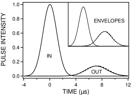
Figure 8: Propagation of a Gaussian-shaped pulse in the EIT experiment. The parameters are as in Fig.7 with $\sigma_{in}=1.5\>\mu s$. The full and dashed lines respectively are the exact intensity-profile of the pulse and the normal form. The location of the two maximums differ by $0.2\>\mu s$ in agreement with the relation $\Delta t_{out}=a/2\sigma_{out}^{2}$. Inset : the corresponding pulse-envelopes for $-5\>\mu s\leq t\leq 15\>\mu s$ .

Fig.8 shows the result obtained with a Gaussian-shaped incident-pulse. $A$ , $\gamma_{ba}$ and $\sigma_{in}$ being given, we have chosen the other parameters in order to reproduce the location and the amplitude of the maximum of the transmitted pulse in the celebrated experiment by Hau et al. ref7 . We then get $\sigma_{out}/\sigma_{in}\approx 1.6$, a broadening consistent with the observations, and $\xi_{out}\approx 0.16$. The asymmetry being very slight, the delay of the maximum is very close to $\tau_{g}$ and $e_{out}(t)$ is well fitted by the normal (Gaussian) form $e_{out}^{(2)}(t)$. A perfect fit is obtained by using the improved form $e_{out}^{(3)}(t)$. The contribution $e_{off}(t)$ associated with $h_{off}(t)$ is actually too small to be visible. Conversely $h_{off}(t)$ will be responsible for the generation of short transients when $e_{in}(t)$ comprises localised defects. As expected and recently discussed about the EIT experiments ref27 , the front of these transients will propagate at the velocity $c$ (instantaneously in our local time picture). Their peak amplitude will be especially large when the defects consist in discontinuities. Consider again a square-shaped incident-pulse, the total duration $2\tau_{p}$ and the amplitude $\eta$ of which are such that its area and its variance equal those of the Gaussian-shaped pulse (Fig.9).

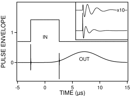
Figure 9: Propagation of a square-shaped pulse in the EIT experiment. Parameters as in the two previous figures. The upper and lower curves are the envelopes of the incident and transmitted pulses. The peak amplitude of the transients is slightly smaller than its theoretical value due to the finite time-resolution of the computations (0.4 ns). Inset : the first transient expanded on a $0.2\mu s$ time-interval (bottom) and the same ($\times 10$) after passage through a $1^{st}$ order filter of time-constant $\sigma_{out}/100$ (top). Such a filtering does not significantly affect the smooth part of the pulse which keeps very close to that obtained with an incident Gaussian-shaped pulse but reduces the amplitude (resp. the intensity) of the transient by a factor of about 30 (resp. 900).

$e_{off}(t)$ is then easily derived from $h_{off}(t)$. It reads

$$e_{off}(t)=\eta\left[f(t+\tau_{p})-f(t-\tau_{p})\right]$$ (13)

with

$$f(t^{\prime})=U(t^{\prime})-\gamma_{ba}A\int_{0}^{t^{\prime}}\frac{J_{1}(\sqrt{2A\gamma_{ba}x})}{\sqrt{2A\gamma_{ba}x}}\exp\left(-\gamma_{ba}x\right)dx.$$ (14)

Each discontinuity in $e_{in}(t)$ actually originates a large transient. Its initial amplitude is equal to that of the incident pulse and its successive maximums of intensity occur at the instants $j_{1n}^{2}/2A\gamma_{ba}$ later, $j_{1n}$ being the $n^{th}$ zero of $J_{1}(u)$ ref28 . Note that the amplitude of the transients exceeds that of the smooth part of $e_{out}(t)$. In a real experiment however the finite values of the rise and fall times of the incident pulse and of the detection bandwidth will generally limit the importance of the transients. By a deliberate reduction of the detection bandwidth, it is even possible to bring their intensity to a very low level without significantly affecting the delayed Gaussian-like part (see inset of Fig.9).

The results obtained on the model EIT-arrangement hold for an extended class of systems having a transparency-window in a wide absorption profile. They only lie on three assumptions: (i) $\Gamma(\Omega)$ is Lorentzian in the far wings of the absorption profile (ii) the opaque regions are much wider that the transparency-window (iii) the transfer-function does not significantly deviate from the normal form in the transparency-window. The first condition (i) is generally met even when $\Gamma(\Omega)$ is not Lorentzian in its central part. Anyway, it is not essential. If it is not met, the detailed shape of the transients is modified but not their main features (instantaneous transmission, duration proportional to the inverse of the spectral width of the opaque regions). The conditions (ii) and (iii), which are closely related, are met in the EIT experiments when the medium transmission is good at the frequency of the optical carrier (see before) but this is not always sufficient. As a counter-example we consider the experiment achieved by Tanaka et al. in an atomic vapour with a natural transparency-window between two strong absorption lines ref29 . The complex gain-factor reads

$$\Gamma(\Omega)=-\frac{A}{2}\left[\frac{1}{1+i(\Omega+\Delta)/\gamma}+\frac{1}{1+i(\Omega-\Delta)/\gamma}\right]$$ (15)

where $2\Delta$ is the doublet splitting. Despite an apparent similarity, the associated transfer-function dramatically differs from that obtained in EIT when $\Omega_{s}>(\gamma_{ba}-\gamma_{ca})$. Indeed the two involved lines are here purely Lorentzian (not hybrid) and a good transparency at $\Omega=0$ is achieved only if $\Delta\gg\gamma$. We then get $H_{0}\approx\exp\left(-A\gamma^{2}/\Delta^{2}\right)$, $\tau_{g}\approx A\gamma/\Delta^{2}$ , $\sigma^{2}\approx 6A\gamma^{2}/\Delta^{4}$, $a\approx-6A\gamma/\Delta^{4}$ and $\xi\approx-\Delta^{2}/(\gamma^{2}\sqrt{6A})$. Choosing the physical parameters such that $H_{0}$, $\tau_{g}$ and $\sigma^{2}$ equal their values in the EIT experiment , we actually obtain a quite different gain profile with opaque regions whose width is smaller than that of the transparency-window (Fig.10).

Figure 10: . Gain-profile $\lvert H(\Omega)\rvert$ for the two absorption-lines arrangement (full line) compared to the corresponding normal gain-profile $\lvert H^{2(}(\Omega)\rvert$ (dotted line). $H_{0}$, $\tau_{g}$, $\sigma$ and frequency unit as in Fig.7. Inset : envelope of the transmitted pulse for a Gaussian-shaped incident pulse (full line) compared to that obtained with the EIT-arrangement (dotted line). $\sigma_{in}=1.5\>\mu s$

This entails that the approximation $\left|H(\Omega)\right|\approx\left|H^{(2)}(\Omega)\right|$ only works in the immediate vicinity of $\Omega=0$. It is the same for the law $\Phi(\Omega)\propto\Omega$, the skewness being very large ($\xi\approx-7.6$ ). In such conditions, even a Gaussian-shaped pulse is strongly distorted (see inset of Fig.10). In fact the two absorption-lines arrangement allows one to attain large fractional delays $\tau_{g}/\sigma_{in}$ with moderate distortion and broadening but this requires to involve much larger absorption-parameters and to accept a lower transmission. For example, Tanaka et al. succeeded in obtaining $\tau_{g}/\sigma_{in}\approx 13$ with Gaussian-like pulses (see Fig.4c in ref29 ) but the peak-intensity of the transmitted pulse was 75 times smaller than that of the incident pulse. Their results are well reproduced with our two-lines model by taking $A=2.6\times 10^{4}$ and $\Delta/\gamma=110$. We then get $\sigma^{2}/\sigma_{in}^{2}\approx 1/25\ll 1$ and we actually are in a case of low distortion as previously discussed (see Fig.4). However, pulses with discontinuities are excluded. Since $H(\infty)\gg H_{0}$, the resulting transients (not delayed) would indeed be much larger than the delayed part of the transmitted pulse and would obscure it. Moreover, due to the narrowness of the opaque regions, the time scales of the transients and of the delayed part do not considerably differ and it is thus impossible to filter out the former without denaturing the latter.

VI SUMMARY AND DISCUSSION

Privileging the time-domain analysis, we have studied the linear propagation of light pulses, the frequency of which coincides with that of a pronounced maximum in the transmission of the medium. An important point is that substantial pulse-delays are only attained when the corresponding transmission exceeds the minimum one by a very large factor $C$ (contrast). The impulse response of the medium then tends to a normal (Gaussian) form, irrespective of the line profile associated with the transmission peak. The propagation of arbitrarily shaped light-pulses with significant delays and low distortion is possible when the rms duration $\sigma$ of the medium impulse-response is small compared to that of the incident pulse ($\sigma_{in}$), which should itself be small compared to the group delay $\tau_{g}$. The fulfilment of this double condition requires systems where $C$ is extremely large, typically several tens of thousands of $dB$ in a logarithmic scale. Systems with such contrast have actually been used ref2 but, in most slow-light experiments, $C$ ranges from 30 to 600 dB. Significant fractional time-delays $\tau_{g}/\sigma_{in}$ keep attainable with such values of $C$ by using incident pulses, the duration of which is comparable to or smaller than $\sigma$. As the medium impulse-response, the transmitted pulse then tends to acquire a normal (Gaussian) shape whatever its initial shape is. This reshaping is particularly striking when the incident pulse is square-shaped but is reduced to a simple broadening when the latter is itself Gaussian-shaped. Despite its asymptotic character, the normal form generally provides a good approximation of the shape of the transmitted pulse. More precise shapes are obtained by a perturbation method, allowing us in particular to specify how much the delay of the pulse-maximum deviates from the group delay.

All these results have been first established by assuming that the transmission peak is put on an uniform background. We have shown that they also apply when the transmission peak is associated with a transparency window in an absorption-profile of finite width. This however requires that the nearly opaque regions flanking the transparency window be considerably wider than the latter. Other things being equal, there are then no differences between the cases of uniform and non uniform transmission-backgrounds, at least when the envelope of the incident pulse is smooth. Conversely localised defects in this envelope will be responsible for the generation of very short transients which complement the normal (Gaussian) part of the signal. The front of the transients is instantaneously propagated in our local time picture (that is at the velocity $c$ in a dilute sample). In extreme cases, their amplitude may be comparable to that of the delayed signal but, due to their location and their duration, they can easily be eliminated without altering the latter.

The slow and fast light experiments have a common feature. In both cases, the observation of significant effects requires media with a very large contrast between the maximum and the minimum of transmission. This results from the causality principle and implies severe limits to the effects attainable in fast-light experiments, whatever the involved system is ref30 . From this viewpoint the slow-light case is obviously less pathologic and the constraints, although real, are much softer.

VII ACKNOWLEDGEMENTS

Laboratoire PhLAM is Unité Mixte de Recherche de l’Université de Lille I et du CNRS (UMR 8523). CERLA is Fédération de Recherche du CNRS (FR 2416).

References

- (1) S.E. Harris, J.E. Field, and A. Kasapi, Phys. Rev. A 46, R29 (1992).
- (2) A. Kasapi, M. Jain, G.Y. Yin, and S.E. Harris, Phys. Rev. Lett. 74, 2447 (1995).
- (3) A.B. Matsko, O. Kocharovskaya, Y. Rostovtsev, G. R. Welch, A. S. Zibrov, and M. O. Scully, Adv. At. Mol. Opt. Phys. 46, 191 (2001).
- (4) R.W. Boyd and D.J. Gauthier in Progress in Optics, E. Wolf, ed. (Elsevier, 2002), Vol. 43, p.497.
- (5) P.W. Milonni, Fast Light, Slow Light and Left-Handed Light (IOP, 2005).
- (6) M.S. Bigelow, N.N. Lepeshkin, and R.W. Boyd, Phys. Rev. Lett. 90, 113903 (2003).
- (7) L.V. Hau, S.E. Harris, Z. Dutton, and C.H. Behrooz, Nature 397, 594 (1999).
- (8) A.V. Turukhin, V.S. Sudarshanam, M.S. Shahriar, J.A. Musser, B.S. Ham, and P.R. Hemmer, Phys. Rev. Lett. 88, 023602 (2002)
- (9) R. W. Boyd, D. J. Gauthier, A. L. Gaeta, and A. E. Willner, Phys. Rev. A 71, 023801 (2005).
- (10) A.B. Matsko, D.V. Strekalov, and L. Maleki, Optics Express 13, 2210 (2005)
- (11) K. Lee and N.M. Lawandy, Appl. Phys. Lett. 78, 703 (2001).
- (12) D.J. Gauthier, 2nd Annual Summer School, Fitzpatrick Center for Photonics and Communication, Duke University, Durham, N.C. (2004).
- (13) K.Y Song, M. González-Herráez, and L. Thévenaz, Optics Express 13, 82 (2005)
- (14) Y. Okawachi, M.S. Bigelow, J.E. Sharping, Z. Zhu, A. Schweinsberg, D.J. Gauthier, R.W. Boyd, and A.L. Gaeta, Phys. Rev. Lett. 94, 153902 (2005).
- (15) K.Y Song, M. González-Herráez, and L. Thévenaz, Opt. Lett. 30, 1782 (2005).
- (16) M. González-Herráez, K.Y. Song, and L. Thévenaz, Appl. Phys. Lett. 87, 081113 (2005).
- (17) J.E. Sharping, Y. Okawachi, and A.L. Gaeta, Optics Express 13, 6092 (2005).
- (18) N.S. Bukhman, Quant. Electron. 34, 299 (2004).
- (19) A.Papoulis, The Fourier Integral and its Applications (McGraw-Hill 1987).
- (20) M. Abramowitz and I.A. Stegun, Handbook of Mathematical functions (Dover, 1972).
- (21) G. Wunsch, Nachrichtentechnik 6, 244 (1956).
- (22) B. Macke and B. Ségard, Eur. Phys. J. D 23, 121 (2003).
- (23) M. D. Crisp, Phys. Rev. A 1, 1604 (1970).
- (24) L. Casperson and A. Yariv, Phys. Rev. Lett. 26, 293 (1971).
- (25) G.P. Agrawal, Nonlinear Fiber Optics, 3rd Ed. (Academic Press, 2001).
- (26) H.J. Hartmann and A. Laubereau, Opt. Commun. 47, 117 (1983).
- (27) M.D. Stenner, D.J. Gauthier, and M.A. Neifeld, Phys. Rev. Lett. 94, 053902 (2005).
- (28) For an experimental demonstration of these transients, see, e.g., B. Ségard, J. Zemmouri, and B. Macke, Europhys. Lett. 4, 47 (1987).
- (29) H. Tanaka, H. Niwa, K. Hayami, S. Furue, K. Nakayama,T. Kohmoto, M. Kunitomo, and Y. Fukuda, Phys. Rev. A 68, 053801 (2003).
- (30) B. Macke, B Ségard, and F. Wielonsky Phys. Rev. E 72, 035601(R) (2005).