Escape rates in periodically driven Markov processes

Abstract

We present an approximate analytical expression for the escape rate of time-dependent driven stochastic processes with an absorbing boundary such as the driven leaky integrate-and-fire model for neural spiking. The novel approximation is based on a discrete state Markovian modeling of the full long-time dynamics with time-dependent rates. It is valid in a wide parameter regime beyond the restraining limits of weak driving (linear response) and/or weak noise. The scheme is carefully tested and yields excellent agreement with three different numerical methods based on the Langevin equation, the Fokker-Planck equation and an integral equation.

, ,

1 Introduction

Although the solution of the stationary and unbounded Ornstein-Uhlenbeck process has been found long ago, it is not yet possible to give an analytic exact expression that includes time-dependent driving and absorbing boundaries [1, 2]. Yet, such processes with a linear restoring force an a periodic driving which terminate at a prescribed threshold are widely used as models for numerous physical effects. Examples range from rupturing experiments on molecules [3] where the time-dependence is introduced as linear movement of the absorbing boundary up to totally different models like the leaky integrate-and-fire (LIF) model for neuronal spiking events [4, 5, 6, 7, 8]. The latter is the application we primarily think of in this paper. The stochastic variable stands for the cell soma’s electric potential $x(t)$ that is changing due to a great many incoming signals from other neurons. It is thus customary to employ a diffusion approximation for the stochastic dynamics of $x(t)$. The driven abstract LIF model assumes the non-stationary Langevin dynamics (in dimensionless coordinates)

$$\dot{x}(t)=-x(t)+A\cos(\omega t+\phi)+\sqrt{2D}\,\xi(t)$$ (1)

where the process starts at time $t=0$ at $x(0)=x_{0}$ and fires when it reaches the threshold voltage $x=a\equiv 1$. $\xi(t)$ is white Gaussian noise. Here, a sinusoidal stimulus has been chosen for the sake of convenience. The following analysis may easily be extended to general periodic stimuli. The dynamics of the process $x(t)$ is equivalently described by a Fokker-Planck (FP) equation for the conditional probability density function (PDF) $\rho(x,t\mathop{|}x_{0},0)$ in a time-dependent quadratic potential, $U(x,t)=\bigl{(}x-A\cos(\omega t+\phi)\bigr{)}^{2}/2$, reading

$$\frac{\partial}{\partial t}\,\rho=L(t)\rho=\frac{\partial}{\partial x}\,\bigl{(}U^{\prime}(x,t)\rho\bigr{)}+D\frac{\partial^{2}}{\partial x^{2}}\,\rho\>,$$ (2)

with the absorbing boundary and initial conditions

$$\rho(a,t\mathop{|}x_{0},0) =0\quad\text{for all $t$ and $x_{0}$}$$ (3)

$$\rho(x,0\mathop{|}x_{0},0) =\delta(x-x_{0}).$$ (4)

After firing the process immediately restarts at the instantaneous minimum of the potential.

The set of eqs. (1–4) defines our starting point for obtaining the firing statistics of this driven neuron model. Our main objective is to develop an accurate analytical approximation that avoids certain restrictive assumptions of prior attempts. Those, in fact, all involve the use of either of the following limiting approximation schemes such as the limit of linear response theory (i.e. a weak stimulus $A\ll 1$) [7, 9] or the limit of asymptotically weak noise [10, 11, 12, 13, 14]. Our scheme detailed below yields novel analytic and tractable expressions beyond the linear response and weak noise limit; as will be demonstrated, this novel scheme indeed provides analytical formulae that compare very favorably with precise numerical results of the full dynamics in eqs. (1, 2–4). The arguments given for the agreement of the first-passage time distribution also hold for the residence-time [15] which is not further considered here.

2 Reduction to a discrete model

The periodicity of the external driving with the period $T=2\pi/\omega$ allows one to represent the time-dependent solution $\rho(x,t)$ of the Fokker Planck equation in terms of Floquet eigenfunctions and eigenvalues of the Fokker-Planck operator, $v_{i}(x,t)$ and $\mu_{i}$, respectively, [10, 16]

$$-\frac{\partial}{\partial t}v_{i}(x,t)+L(t)v_{i}(x,t)=\mu_{i}v_{i}(x,t),$$ (5)

where the eigenfunctions are periodic in time, integrable in $x$ from $-\infty$ to $a$, and fulfill the absorbing boundary condition at $x=a$

$$v_{i}(a,t)=0.$$ (6)

The time-dependent PDF can be written as a weighted sum of the Floquet eigenfunctions

$$\rho(x,t)=\sum_{i}c_{i}\,v_{i}(x,t)\,\exp(\mu_{i}t)$$ (7)

where the coefficients $c_{i}$ are determined by the initial PDF. Note that because of the absorbing boundary condition at $x=a$ the total probability is not conserved and therefore all Floquet eigenvalues have a non-vanishing negative real part.

The first main assumption that we impose concerns the value of the potential at the boundary: The minimum of the potential must always belong to the “allowed” region left of the threshold, and, moreover, the potential difference between threshold and minimum, denoted by $\Delta U(t)$, must always be larger than at least a few $D$, i.e. $\Delta U(t)/D>4$. This assumption implies an exponential time-scale separation between the average time $\tau_{\kappa}$ in which the threshold is reached from the minimum of the potential compared to the time $\tau_{r}$ of the deterministic relaxation towards the potential minimum. In the dimensionless units used here $\tau_{r}=1$. For the Floquet spectrum this implies the presence of a large gap between the first eigenvalue $\mu_{1}$ which is of the same order as $-1/\tau_{\kappa}$ and the higher ones which are of the order $-1$ or smaller. After a short initial time of the order $1$, all contributions from higher Floquet eigenvalues can be neglected and only the first one survives:

$$\rho(x,t)\approx v_{1}(x,t)\,\exp(\mu_{1}t)$$ (8)

In general, the Floquet eigenfunctions and the corresponding eigenvalues are difficult to determine. A formal expansion in terms of the instantaneous eigenfunctions $\psi_{i}(x,t)$ of $L(t)$ fulfilling

$$L(t)\psi_{k}(x,t)=\lambda_{k}(t)\psi_{k}(x,t)$$ (9)

is always possible though not always helpful

$$v_{i}(x,t)=\sum_{k}d_{ik}(t)\psi_{k}(x,t).$$ (10)

The periodicity of $v_{i}(x,t)$ and $\psi_{k}(x,t)$ implies that the coefficients $d_{ik}(t)$ also are periodic functions of time. Expansion (10), together with the Floquet equation (5), yields a coupled set of ordinary differential equations for the coefficients $d_{ik}(t)$ [17]

$$\dot{d}_{ik}(t)-\left(\lambda_{k}(t)-\mu_{i}\right)d_{ik}(t)=\sum_{l}d_{il}(t)\Bigl{\langle}\frac{\partial}{\partial t}\varphi_{k}(t),\psi_{l}(t)\Bigr{\rangle},$$ (11)

where $\varphi_{k}(x,t)$ denotes the instantaneous eigenfunction of the backward operator $L^{+}(t)$ belonging to the eigenvalue $\lambda_{k}(t)$

$$L^{+}(t)\varphi_{k}(x,t)=\lambda_{k}(t)\varphi_{k}(x,t).$$ (12)

The eigenfunctions $\psi_{k}(x,t)$ and $\varphi_{k}(x,t)$ constitute a bi-orthogonal set of functions that always can be normalized such that

$$\left\langle\varphi_{l}(t),\psi_{k}(t)\right\rangle=\delta_{kl}.$$ (13)

Here, the scalar product $\left\langle f,g\right\rangle$ is defined as the integral over the real axis up to the threshold:

$$\left\langle f,g\right\rangle=\int_{-\infty}^{a}dx\>f(x)g(x)$$ (14)

With our second assumption we require that the driving frequency $\omega$ is small compared to the relaxation rate in the parabolic potential. Under this condition, the matrix elements $\left\langle\partial\varphi_{k}(t)/\partial t,\psi_{l}(t)\right\rangle$ that are proportional to the frequency $\omega$ are also small and may be neglected to lowest order in the equations for the coefficients $d_{ik}(t)$ [17]. The resulting equations are uncoupled and readily solved to yield with the periodic boundary conditions

$$d_{1k}(t)\approx\delta_{1k}\exp\Bigl{(}\int_{0}^{t}dt^{\prime}\,\lambda_{1}(t^{\prime})-\mu_{1}t\Bigr{)},$$ (15)

where $\mu_{1}=\frac{1}{T}\int_{0}^{T}\lambda_{1}(t)\,dt$ follows from the periodicity of $d_{11}(t)$. Together with eqs. (8) and (10) we obtain for the long-time behavior of the PDF

$$\rho(x,t)\approx\exp\Bigl{(}\int_{0}^{t}dt^{\prime}\,\lambda_{1}(t^{\prime})\Bigr{)}\>\psi_{1}(x,t).$$ (16)

Note, that the first Floquet eigenvalue has canceled. The lowest instantaneous eigenfunctions $\psi_{1}(x,t)$ and $\varphi_{1}(x,t)$ are related by

$$\psi_{1}(x,t)=\varphi_{1}(x,t)\rho_{0}(x,t),$$ (17)

where

$$\rho_{0}(x,t)\propto\exp\bigl{(}-U(x,t)/D\bigr{)}.$$ (18)

For the corresponding eigenvalue $\lambda_{1}(t)$ we find from (9)

$$\lambda_{1}(t)=\frac{\int_{-\infty}^{a}dx\>\varphi_{1}(x,t)L(t)\varphi_{1}(x,t)\rho_{0}(x,t)}{\int_{-\infty}^{a}dx\>\varphi_{1}^{2}(x,t)\rho_{0}(x,t)}\;.$$ (19)

An explicit expression, valid for high potential differences, can be given after linearization of $U$ about $a$

$$\varphi_{1}(x,t)=1-\exp\bigl{(}(x-a)U^{\prime}(a,t)/D\bigr{)}$$ (20)

which gives for $\lambda_{1}(t)$

$$\lambda_{1}(t)=-\frac{\Delta U(t)}{D}\;\frac{1-\operatorname{erf}\bigl{(}\sqrt{\Delta U(t)/D}\,\bigr{)}}{1-\exp(-\Delta U(t)/D)}\;.$$ (21)

where $\operatorname{erf}(z)$ is the error function.

The waiting-time probability [18] can be expressed as

$$P(t)=\int_{-\infty}^{a}dx\,\varphi_{1}(x,t)\rho(x,t)=\exp\bigl{(}\int_{0}^{t}dt^{\prime}\,\lambda_{1}(t^{\prime})\bigr{)}\>.$$ (22)

Therefore, the eigenvalue $\lambda_{1}(t)$ coincides with the negative of the time-dependent escape rate $\kappa(t)$.

With the expression (21) for the escape rate we can calculate the property of interest, namely the PDF for the first-passage time (FPT) of the attracting ”integrating” state that covers the domain $-\infty<x(t)<a$. The FPT-PDF is given by the negative rate of change of the waiting time probability, i.e.

$$g(t)=-\frac{dP(t)}{dt}=\kappa(t)\>\exp\Bigl{(}-{\int_{0}^{t}}\kappa(t^{\prime})\,dt^{\prime}\Bigr{)}\>,$$ (23)

The quantitative validity of these expressions for an extended parameter regime will be checked next.

3 Numerical analysis

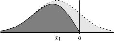
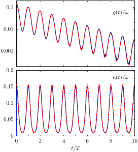
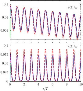
Figure 1: The transition probabilities $p(x_{i{+}1},t+\delta t\mathop{|}x_{i},t)$ (black line) and $N_{1}(x_{i{+}1},t+\delta t\mathop{|}\allowbreak x_{i},t)$ (dashed line) from $x_{i}$ for a single time-step, with and without the absorbing boundary, respectively. The vertical line indicates the boundary.

Figure 2: First-passage time density $g(t)$ (upper) and rate $\kappa(t)$ (lower plots) as functions of time. Displayed are all three numerical methods we used for testing (solid lines) and the approximation based on (21) (dashed lines). The parameters in the left plots, $\Delta U(t)/D\in[5,8]$ and $\omega=0.05$, are chosen to yield a very good approximation of the rate by (21). The right plots display extreme parameters, $\Delta U(t)/D\in[3,8]$ and $\omega=0.5$, where no good approximation of the rate can be expected. In both cases $\phi=0$.

We implemented three different numerical methods to obtain both the FPT-PDF and the rate in order to have a reliable basis for comparison with the analytical expression (21). The first method performs explicit time-steps of the Langevin equation (1). We used an elaborate technique for the time-integration of the fluctuating force $\xi(t)$. For points away from the threshold $a$ it is sufficient to take a normal distributed random variable for the displacement due to $\xi(t)$. Quite the contrary in the vicinity of the absorbing boundary. Here, the integral of $\xi(t)$ rather behaves like a Wiener process with absorbing boundary, as illustrated in Fig. 2. The appropriate transition distribution, is known analytically as the weighted difference between two normal distributions [1]

$$\begin{split}p(x_{i{+}1},t+\delta t\mathop{|}x_{i},t)&=N_{1}(x_{i{+}1},\delta t\mathop{|}x_{i},0)-N_{2}(x_{i{+}1},\delta t\mathop{|}x_{i},0)\\ &=:N_{1}(x_{i{+}1},\delta t\mathop{|}x_{i},0)\big{(}1-P_{\text{out}}(x_{i{+}1},x_{i},\delta t)\big{)}\end{split}$$ (24)

The multiplication on the right-hand side stands for a logical AND that leads to a correction step in the algorithm. First, a new position $x_{i{+}1}$ is proposed according to the normal distribution density $N_{1}$. With the probability $P_{\text{out}}(x_{i{+}1},x_{i},\delta t)$ the trajectory has already crossed the boundary during this time-step $\delta t$ from $x_{i}$ to $x_{i{+}1}$ and, therefore, is to be ended. The explicit forms of $N_{1}$ and $N_{2}$ give

$$P_{\text{out}}(x_{i{+}1},x_{i},\delta t)=\frac{N_{2}}{N_{1}}=\exp\Bigl{(}-\frac{1}{D\delta t}(a-x_{i{+}1})(a-x_{i})\Bigr{)}\>.$$ (25)

The same formula has been given by [19] but with a different reasoning.

In order to get the correctly normalized FPT-PDF $g(t)$ we counted the number of trajectories hitting the absorbing boundary within the interval $[t,t+\delta t)$. The FPT-PDF is then estimated by this number divided by $\delta t$ and by the total number of trajectories. The rate is given by

$$\kappa(t)=g(t)/P(t),$$ (26)

where $1-P(t)$ is estimated by the number of trajectories that have escaped up to time $t$, divided by the total number of trajectories.

For the second numerical method we have solved the FP equation (2) using a Chebychev collocation method to reduce the problem to a coupled system of ordinary differential equations [13, 20]. This gives $P(t)$ as the integral of $\rho(x,t)$ from $-\infty$ to $a$. The FPT-PDF in the figures is then calculated according to eq. (23), and the rate again by (26).

The third method solves Ricciardi’s integral equation for the FPT-PDF and is detailed in [21, 22]. For employing his algorithm the process must be transformed into a stationary Ornstein-Uhlenbeck process with a moving absorbing boundary

$$S(t)=a-\frac{A}{1+\omega^{2}}\Bigl{[}\cos(\omega t+\phi)+\omega\sin(\omega t+\phi)-e^{-t}\Bigr{]}\>.$$ (27)

All three methods provide practically identical results as can be seen in Figs. 2 and 3. The results for the FPT-PDF and for the rate all collapse into one single line. Differences between the numerical methods, e.g. fluctuations in the histogram of the Langevin equation method are visible only in the plots of the relative errors (Fig. 3 middle and lower rows).

Figure 2 shows that the FPT-PDF is extremely well approximated by expression (21) for the rate $\kappa(t)$. In the left plots we used quite a high barrier with quite slow driving compared to the time-scale $\tau_{r}$ of the process. Good agreement is thus expected. In the right plots we show the situation with extreme parameters. The lower barrier height $\Delta U_{\text{min}}/D$ goes down to $3$ where a rate-description is unlikely to suffice. Moreover, the driving is faster, $\omega=0.5$. The system cannot follow the driving instantaneously, and we find a shift in the maximum of the FPT-PDF to later times. Under these conditions it is impressing how good the novel approximation still works.

A more delicate measure for the errors of the approximation are the rate $\kappa(t)$ itself and its relative deviation from the three numerically calculated rates. Both can be seen in Fig. 3. The upper row of plots shows the approximation error of the rate for the same two parameter sets as in Fig. 2. Especially at the maximum the rate is over-estimated. This leads to a faster decay of the FPT-PDF which is scarcely visible in Fig. 2. Also, the shift of the maxima (indicated by vertical lines) can be observed. It is negligibly small for $\omega=0.05$ but more pronounced for $\omega=0.5$.

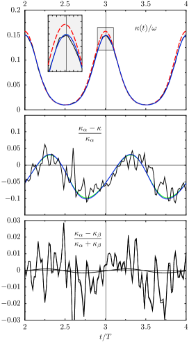
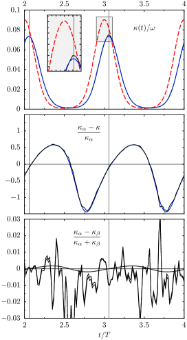
Figure 3: Comparison of the numerical rates and the novel approximation from eq. (21). The respective parameters in the left/right plots are the same as in Fig. 2. Upper plots: The numerically determined rates are displayed as solid lines: Langevin equation simulations (black); Fokker-Planck equation (blue); Ricciardi’s integral equation (green). The theoretical approximation $\kappa(t)$ from eq. (21) is displayed as the red dashed line. Middle plots: Relative error of the approximation $\kappa(t)$ with respect to each numerical rate $\kappa_{\alpha}(t)$ (with the same color coding as above). Lower plots: Errors of the numerical rates with respect to each other. The thin vertical lines indicate the positions of the numerical rates’ maxima.

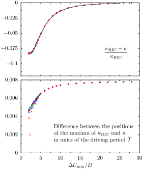
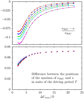
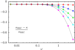
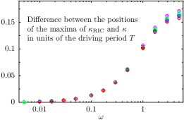
Figure 4: Relative error and relative time-shift of the rate (21). As the basis of comparison we used the rate $\kappa_{\text{RIC}}$ obtained by solving Ricciardi’s integral equation [21] at times $t>\tau_{r}$ where it has become periodic. Upper plots: The error relative to $\kappa_{\text{RIC}}$ evaluated at the maxima of $\kappa_{\text{RIC}}$. Shown are data for $(\Delta U_{\text{max}}/D-\Delta U_{\text{min}}/D)\in(0.1,1,2,3,5)$, from top to bottom with the colors $(\text{red},\text{green},\text{blue},\text{cyan},\text{magenta})$, and the phase $\phi\in(0,\pi/2,\pi)$ with the symbols $(\boldsymbol{\times}$, $\circ$, $\boldsymbol{+})$. In the left panel the driving is slow, $\omega=0.05$, in the right it is fast, $\omega=0.5$. Note that the relative error is of the same order of magnitude for slow and for fast driving. A dependence on the phase $\phi$ cannot be observed. Lower plots: The difference of the maxima’s position of $\kappa_{\text{RIC}}$ and rate (21) in units of the period $T$, again for $\omega=0.05$ (left panel) and $\omega=0.5$ (right panel). Color and symbol codings are the same as above.

Figure 5: Relative error and relative time-shift of the maxima as a function of $\omega$. For all data points $\Delta U_{\text{min}}/D=5$. The color and symbol codings for $\Delta U_{\text{max}}/D$ and $\phi$ are the same as in Fig. 5. For fast driving the relative error starts depending on the interval length of $\Delta U(t)/D$.

In the middle row of Fig. 3 a systematic error of the approximation becomes visible. The relative error with respect to the numerical results behaves roughly sinusoidally with a phase-shift of $\pi/2$ relative to the driving and with an additional constant offset. For the instantaneous rate expression (19) to be valid it is necessary that the driving signal is sufficiently slow. If this assumption is violated then a rate can still be defined if the barrier is sufficiently high. But in addition to the leading term $d_{11}(t)$ in (10) the higher instantaneous eigenfunctions must be taken into account. The coupling to the coefficients $d_{1k}(t)$ is induced by the matrix elements $\langle\dot{\phi}_{k}(t),\psi_{l}(t)\rangle$, see eq. (11), containing a time derivative that introduces non-adiabatic corrections to the rate and, consequently, to the statistics of the FPT.

It is quite astonishing, that the huge relative error in the right middle plot of Fig. 3 leads to such a good result in Fig. 2. The explanation for this is that the FPT-PDF (23) uses the time-integrated rate. Therefore, errors are important only where the rate is large. A closer look on the plot shows that around the maxima of the rate the relative error is comparably small. Because the errors are linear in time around the rate’s maxima they cancel out when integrated over time in (23). The same is valid for the residence time whose PDF also contains integrals of the rate [15, 23].

Figure 5 shows this relative error of $\kappa(t)$ at the maxima of the numerically obtained rate as a function of the barrier height. Again, two different driving frequencies are given. In both cases the relative error has the same order of magnitude, and thus explains why both parameter sets in Fig. 2 yield good approximations.

Finally, we would like to point the reader’s attention to the limitations of the linear response approximation. For linear response the parameter ratio $A/D$ needs to be small. In our validating example in Fig. 2 (left plots) it takes on the value $A/D=1.5$. Thus, our approximation scheme is valid beyond the linear response limit.

The time-scale of the driving force is mainly restricted by the relaxation time-scale $\tau_{r}$ and much less by the magnitude of the rate itself. There is no restriction on the relative magnitudes of $\kappa$ and $T$. Instead, both $\omega$ and $\kappa$ have to be sufficiently small. Fig. 5 indicates that both the relative error and the time-shift of the maxima’s positions are modest for $\omega<0.1$.

4 Conclusions

By reference to a discrete Markovian dynamics for the corresponding full space-continuous stochastic process we succeeded in obtaining an analytical approximation for the time-dependent escape rate which can be used for calculating first-passage time statistics. This result is valid beyond the restraining limits of linear response or asymptotically weak noise and of adiabatically slow driving.

We checked our findings using simulations of the Langevin equation (1) and numerical solutions of the equivalent FP equation in (2) and of the integral equation in [21]. We found an impressive agreement for the first-passage time density and a good match for the rate which is the more delicate property for comparison.

Finally, we note that our method is not restricted to a periodic forcing but applies also to arbitrary drive functions. However, in the oscillatory case some of the approximation errors cancel out. This leads to useful results in extreme parameter regimes where agreement cannot be expected a priori.

This work has been supported by the Deutsche Forschungsgemeinschaft via project HA1517/13-4 and SFB-486, projects A10 and B13.

References

- [1] N. S. Goel and N. Richter-Dyn, Stochastic Models in Biology, Academic Press, New York, 1974.
- [2] P. Hänggi, P. Talkner, and M. Borkovec, Rev. Mod. Phys. 62 (1990) 251.
- [3] G. Hummer and A. Szabo, Biophys. J. 85 (2003) 5.
- [4] N. Fourcaud and N. Brunel, Neural Comp. 14 (2002) 2057.
- [5] H. C. Tuckwell, Stochastic Processes in the Neurosciences, SIAM, Philadelphia, 1989.
- [6] L. Ricciardi, Diffusion Processes and Related Topics in Biology, Springer, Berlin, 1977.
- [7] B. Lindner, J. Garciía-Ojalvo, A. Neiman, and L. Schimansky-Geier, Phys. Rep. 392 (2004) 321.
- [8] P. Lansky, Phys. Rev. E 55 (1997) 2040.
- [9] B. Lindner and L. Schimansky-Geier, Phys. Rev. Lett. 86 (2001) 2934.
- [10] L. Gammaitoni, P. Hänggi, P. Jung, and F. Marchesoni, Rev. Mod. Phys. 70 (1998) 223.
- [11] J. Lehmann, P. Reimann, and P. Hänggi, Phys. Rev. Lett. 84 (2000) 1639.
- [12] A. Nikitin, N. G. Stocks and A. R. Bulsara, Phys. Rev. E 68 (2003) 016103.
- [13] J. Lehmann, P. Reimann, and P. Hänggi, Phys. Rev. E 62 (2000) 6282.
- [14] J. Lehmann, P. Reimann, and P. Hänggi, Phys. Stat. Sol. (B) 237 (2003) 53.
- [15] M. Schindler, P. Talkner, and P. Hänggi, Phys. Rev. Lett. 93 (2004) 048102.
- [16] P. Jung, Phys. Rep. 234 (1993) 175.
- [17] P. Talkner, New J. Phys. 1 (1999) 4.
- [18] P. Talkner and J. Łuczka, Phys. Rev. E 69 (2004) 046109.
- [19] J. Honerkamp, Stochastische Dynamische Systeme, VCH Verlag, Weinheim, 1990.
- [20] M. Berzins and P. M. Dew, ACM Trans. Math. Software 17 (1991) 178.
- [21] E. Di Nardo, A. G. Nobile, E. Pirozzi, L. M. Ricciardi, Adv. Appl. Probab. 33 (2001) 435.
- [22] A. Buonocore, A. G. Nobile, and L. M. Ricciardi, Adv. Appl. Probab. 19 (1987) 784.
- [23] P. Talkner, Physica A 325 (2003) 124.