General stability criterion of two-dimensional inviscid parallel flow

Abstract

A more restrictively general stability criterion of two-dimensional inviscid parallel flow is obtained analytically. First, a sufficient criterion for stability is found as either $-\mu_{1}<\frac{U^{\prime\prime}}{U-U_{s}}<0$ or $0<\frac{U^{\prime\prime}}{U-U_{s}}$ in the flow, where $U_{s}$ is the velocity at inflection point, $\mu_{1}$ is the eigenvalue of Poincaré’s problem. Second, this criterion is generalized to barotropic geophysical flows in $\beta$ plane. Based on the criteria, the flows are are divided into different categories of stable flows, which may simplify the further investigations. And the connections between present criteria and Arnol’d’s nonlinear criteria are discussed. These results extend the former criteria obtained by Rayleigh, Tollmien and Fjørtoft and would intrigue future research on the mechanism of hydrodynamic instability.

The stability due to shear in the flow is one of the fundamental and the most attracting problems in many fields, such as fluid dynamics, astrophysical fluid dynamics, oceanography, meteorology et al. The shear instability has been intensively investigated, which is to the greatly helpful understanding of other instability mechanisms in complex shear flows. For the inviscid parallel flow with horizontal velocity profile of $U(y)$, the general way is to investigate the growth of linear disturbances by means of normal mode expansion, which leads to the famous Rayleigh’s equation Rayleigh (1880). Using this equation, Rayleigh Rayleigh (1880) first proved a necessary criterion for instability, i.e., Inflection Point Theorem. Then, Fjørtoft Fjørtoft (1950) found a stronger necessary criterion for instability. These criteria are well known and have been applied to understanding the mechanism of hydrodynamic instability Drazin and Reid (1981); Huerre and Rossi (1998); Criminale et al. (2003). Unfortunately, both criteria are only necessary criteria for instability, except for some special cases of the symmetrical or monotone velocity profiles. Tollmien Tollmien (1936) gave a heuristic result that the criteria are also sufficiency for instability in these special cases.

The stable criteria also provide a way to categorize the velocity profiles of the flows. According to Rayleigh’s criterion, the flows are stable if $U^{\prime\prime}(y)\neq 0$, where $U^{\prime\prime}(y)$ denotes $d^{2}U/dy^{2}$. And according to Fjørtoft’s criterion, there is another kind of stable flows if $U^{\prime\prime}(U-U_{s})>0$, where $U_{s}$ is the velocity at the inflection point $U^{\prime\prime}_{s}=0$. Then if $U^{\prime\prime}(U-U_{s})<0$, can the flow still be stable? Is there another kind of stable flows besides the above flows? To answer these questions, a more restrictive criterion is needed. And the criterion itself is important for both theoretic researches and real applications. The aim of this letter is to obtain such a stability criterion. and other instabilities may be understood via the investigation here.

For this purpose, Rayleigh’s equation for an inviscid parallel flow is employed Rayleigh (1880); Drazin and Reid (1981); Huerre and Rossi (1998); Schmid and Henningson (2000); Criminale et al. (2003). For a parallel flow with mean velocity $U(y)$, the streamfunction of the disturbance expands as a series of waves (normal modes) with real wavenumber $k$ and complex frequency $\omega=\omega_{r}+i\omega_{i}$, where $\omega_{i}$ denotes the grow rate of the waves. The flow is unstable if and only if $\omega_{i}>0$. We study the stability of the disturbances by investigating the growth rate of the waves, this method is known as normal mode method. The amplitude of waves, namely $\phi$, satisfies

$$(\phi^{\prime\prime}-k^{2}\phi)-\frac{U^{\prime\prime}}{(U-c)}\phi=0,$$ (1)

where $c=\omega/k=c_{r}+ic_{i}$ is the complex phase speed. The real part of complex phase speed $c_{r}=\omega_{r}/k$ is the wave phase speed. In fact, Rayleigh’s equation is the vorticity equation of the disturbance Drazin and Reid (1981); Huerre and Rossi (1998). This equation is to be solved subject to homogeneous boundary conditions

$$\phi=0\,\,at\,\,y=a,b.$$ (2)

There are three main categories of boundaries: (i) enclosed channels with both $a$ and $b$ being finite, (ii) boundary layer with either $a$ or $b$ being infinite, and (iii) free shear flows with both $a$ and $b$ being infinite.

It is obvious that the criterion for stability is $\omega_{i}=0$ ($c_{i}=0$), for that the complex conjugate quantities $\phi^{*}$ and $c^{*}$ are also a physical solution of Eq.(1) and Eq.(2). Multiplying Eq.(1) by the complex conjugate $\phi^{*}$ and integrating over the domain $a\leq y\leq b$, we get the following equations

$$\int_{a}^{b}[(\|\phi^{\prime}\|^{2}+k^{2}\|\phi\|^{2})+\frac{U^{\prime\prime}(U-c_{r})}{\|U-c\|^{2}}\|\phi\|^{2}]\,dy=0$$ (3)

and

$$c_{i}\int_{a}^{b}\frac{U^{\prime\prime}}{\|U-c\|^{2}}\|\phi\|^{2}\,dy=0.$$ (4)

Rayleigh used only Eq.(4) to prove his theorem. Fjørtoft noted that Eq.(3) should also be satisfied, then he obtained his necessary criterion. To find a more sufficient criterion, we shall investigate the conditions for $c_{i}=0$. Unlike the former investigations, we consider this problem in a totally different way: if the velocity profile is stable ($c_{i}=0$), then the hypothesis $c_{i}\neq 0$ should result in contradictions in some cases. Following this, some more restrictive criteria can be obtained.

To find a stronger criterion, we need to estimate the ratio of $\int_{a}^{b}\|\phi^{\prime}\|^{2}dy$ to $\int_{a}^{b}\|\phi\|^{2}dy$. This is known as Poincaré’s problem:

$$\int_{a}^{b}\|\phi^{\prime}\|^{2}dy=\mu\int_{a}^{b}\|\phi\|^{2}dy,$$ (5)

where the eigenvalue $\mu$ is positive definition for any $\phi\neq 0$. The smallest eigenvalue value, namely $\mu_{1}$, can be estimated as $\mu_{1}>(\frac{\pi}{b-a})^{2}$, like Tollmien Tollmien (1936) did.

Then using Poincaré’s relation Eq.(5), a new stability criterion may be found: the flow is stable if $-\mu_{1}<\frac{U^{\prime\prime}}{U-U_{s}}<0$ everywhere.

To get this criterion, we introduce an auxiliary function $f(y)=\frac{U^{\prime\prime}}{U-U_{s}}$, where $f(y)$ is finite at the inflection point. We will prove the criterion by two steps. At first, we prove proposition 1: if the velocity profile is subject to $-\mu_{1}<f(y)<0$, then $c_{r}\neq U_{s}$.

Proof: Since $-\mu_{1}<f(y)<0$, then

$$-\mu_{1}<\frac{U^{\prime\prime}}{U-U_{s}}=\frac{U^{\prime\prime}(U-U_{s})}{(U-U_{s})^{2}}\leq\frac{U^{\prime\prime}(U-U_{s})}{(U-U_{s})^{2}+c_{i}^{2}}.$$ (6)

Substitution of $c_{r}=U_{s}$ and Eq.(6) into Eq.(3) results in

$$\int_{a}^{b}[\|\phi^{\prime}\|^{2}+k^{2}\|\phi\|^{2}+\frac{U^{\prime\prime}(U-U_{s})}{\|U-c\|^{2}}\|\phi\|^{2}]\,dy>0.$$ (7)

This contradicts Eq.(3). So proposition 1 is proved.

Then, we prove proposition 2: if $-\mu_{1}<f(y)<0$ and $c_{r}\neq U_{s}$, there must be $c_{i}^{2}=0$.

Proof: If $c_{i}^{2}\neq 0$, then multiplying Eq.(4) by $(c_{r}-U_{t})/c_{i}$, where the arbitrary real constant $U_{t}$ does not depend on $y$, and adding the result to Eq.(3), it satisfies

$$\int_{a}^{b}[(\|\phi^{\prime}\|^{2}+k^{2}\|\phi\|^{2})+\frac{U^{\prime\prime}(U-U_{t})}{\|U-c\|^{2}}\|\phi\|^{2}]\,dy=0.$$ (8)

But the above Eq.(8) can not hold for some special $U_{t}$. For example, let $U_{t}=2c_{r}-U_{s}$, then there is $(U-U_{s})(U-U_{t})<\|U-c\|^{2}$, and

$$\frac{U^{\prime\prime}(U-U_{t})}{\|U-c\|^{2}}=f(y)\frac{(U-U_{s})(U-U_{t})}{\|U-c\|^{2}}>-\mu_{1}.$$ (9)

This yields

$$\int_{a}^{b}\{\|\phi^{\prime}\|^{2}+[k^{2}+\frac{U^{\prime\prime}(U-U_{t})}{\|U-c\|^{2}}]\|\phi\|^{2}\}dy>0,$$ (10)

which also contradicts Eq.(8). So proposition 2 is also proved.

Using ’proposition 1: if $-\mu_{1}<f(y)<0$ then $c_{r}\neq U_{s}$’ and ’proposition 2: if $-\mu_{1}<f(y)<0$ and $c_{r}\neq U_{s}$ then $c_{i}=0$’, we find a stability criterion. If the velocity profile satisfies $-\mu_{1}<\frac{U^{\prime\prime}}{U-U_{s}}<0$ everywhere in the flow, it is stable. Moreover, the above proof is still valid for $0<f(y)$, which is equivalent to Fjørtoft’s criterion. Thus we have the following theorem.

Theorem 1: If the velocity profile satisfies either $-\mu_{1}<\frac{U^{\prime\prime}}{U-U_{s}}<0$ or $0<\frac{U^{\prime\prime}}{U-U_{s}}$, the flow is stable.

This criterion is more restrictive than Fjørtoft’s criterion. As known from Fjørtoft’s criterion, the necessary condition for instability is that the base vorticity $\xi=-U^{\prime}$ has a local maximal in the profile. Noting that $U^{\prime\prime}/(U-U_{s})\approx\xi_{s}^{\prime\prime}/\xi_{s}$ near the inflection point, where $\xi_{s}$ is the vorticity at inflection point, it means that the base vorticity $\xi$ must be convex enough near the local maximum for instability, i.e., the vorticity should be concentrated somewhere in the flow for instability. A simple example can be given by following Tollmien’s way Tollmien (1936). As shown in Fig.1, there are three vorticity profiles within the interval $-1\leq y\leq 1$, which have local maximal at $y=0$. Profile 2 ($U=-2\sin(\pi y/2)/\pi$) is neutrally stable, while profile 1 ($U=-\sin(y)$) and profile 3 ($U=-\sin(2y)/2$) are stable and unstable, respectively.

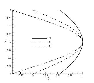
Figure 1: Vorticity profiles within the interval $-1\leq y\leq 1$. Profile 2 ( $\xi=\cos(\pi y/2)$, dashed) is neutrally stable, while profile 1 ($\xi=\cos(y)$, solid) and profile 3 ($\xi=\cos(2y)$, dash doted) are stable and unstable, respectively.

Moreover, the stabile criterion for the parallel inviscid flows can be applied to the barotropic geophysical flows in $\beta$ plane, like Kuo did Kuo (1949). This is a generalized stable criterion, we state it as a new theorem.

Theorem 2: The flow is stable, if the velocity profile satisfies either $-\mu_{1}<\frac{U^{\prime\prime}-\beta}{U-U_{s}}<0$ or $0<\frac{U^{\prime\prime}-\beta}{U-U_{s}}$ in the flow, where $U_{s}$ is the velocity at the point $U^{\prime\prime}=\beta$.

The criteria proved above may shed light on the investigation of vortex dynamics. Both Theorem 1 and Fig.1 show that it is the vorticity profile rather than the velocity profile that dominates the stability of the flow. This means that the distribution of vorticity dominates the shear instability in parallel inviscid flow, which is essential to understanding the role of vorticity in fluid. So an unstable flow might be controlled just by adjusting the vorticity distribution according to present results. This is an very fascinating problem, but can not be discussed in detail here.

To show the power of the criteria obtained above, we consider the stability of velocity profile $U=\tanh(\alpha y)$ within the interval $-1\leq y\leq 1$, where $\alpha$ is a constant. This velocity profile is an classical model of mixing layer, and has been investigated by many researchers (see Huerre and Rossi (1998); Schmid and Henningson (2000); Criminale et al. (2003) and references therein). Since $U^{\prime\prime}(U-U_{s})=-2\alpha^{2}\tanh^{2}(\alpha y)/\cosh^{2}(\alpha y)<0$ for $-1\leq y\leq 1$, it might be unstable for any $\alpha$ according to both Rayleigh’s and Fjørtoft’s criteria. But it can be derived from Theorem 1 that the flow is stable for $\alpha^{2}<\pi^{2}/8$. For example, we choose $\alpha_{1}=1.1$ and $\alpha_{2}=1.3$ for velocity profiles $U_{1}(y)$ and $U_{2}(y)$. The growth rate of the profiles can be obtained by Chebyshev spectral collocation method Schmid and Henningson (2000) with 100 collocation points, as shown in Fig.2. It is obvious that $c_{i}=0$ for $U_{1}$ and $c_{i}>0$ for $U_{2}$, which agrees well with the criteria obtained above. This is also a counterexample that Fjørtoft’s criterion is not sufficient for instability. So this new criterion for stability is more useful in real applications.

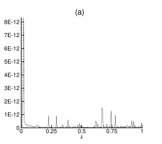
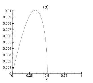
Figure 2: Growth rate $\omega_{i}$ as an function of wavenumber $k$, (a) for $U_{1}=\tanh(1.1y)$, (b) for $U_{2}=\tanh(1.3y)$, both within the interval $-1\leq y\leq 1$.

The present stable criteria give a affirmative answer to the questions at the beginning, i.e., there are some stable flows if $U^{\prime\prime}(U-U_{s})<0$. Based on the former criteria, the velocity profiles can be categorized as follows: (i) without inflection point (Reyleigh’s criterion), (ii) $f(y)>0$ (Fjørtoft’s criterion), and (iii) $\mu_{1}<f(y)<0$ (present criterion). Then the flow might be unstable only for $f(y)<\mu_{1}$ and $f(y)$ changing sign within the interval. However, if $f(y)$ changes sign somewhere within the interval $[a,b]$, then the flow is stable. For that $f(y)$ changing sign implies $U^{\prime\prime\prime}_{s}=0$ but $U^{\prime\prime\prime\prime}_{s}\neq 0$, so $U^{\prime\prime}$ does not change sign near the inflection point. Thus $c_{i}$ must vanish in Eq.(4), i.e., the flow is stable for $f(y)$ changing sign within the interval. In this way, the flow might be unstable only for $f(y)<\mu_{1}$ somewhere, which will intrigue further studies on this problem. In fact, there are still stable flows if $\mu_{1}<f(y)$ is violated.

Recall the proof of theorem 1, it is found that the following Rayleigh’s quotient $I(f)$ plays a key role in determination the stability of the flows.

$$I(f)=\min_{\phi}\frac{\int_{a}^{b}[\,\|\phi^{\prime}\|^{2}+f(y)\|\phi\|^{2}\,]\,dy}{\int_{a}^{b}\|\phi\|^{2}}$$ (11)

Noting that the proof of theorem 1 is still valid in the case of $I(f)>0$. We have such result: the flows are stable if $I(f)>0$. Though this criterion is more restrictive than that in theorem 1, it is inconvenient for the real applications due to unknown value of Rayleigh’s quotient $I(f)$. Theorem 1 is more convenient for the real applications in different research fields.

The idea of categorization the velocity profiles of the flows may simplify the investigation of stability problem. It can be seen from Rayleigh’s equation Eq.(1) that the stability of profile $U(y)$ is not only Galilean invariant, but also independent from the the magnitude of $U(y)$ due to linearity. So the stability of $U(y)$ is the same as that of $AU(y)+B$, where $A$ and $B$ are any arbitrary nonzero real numbers. As the value of $U^{\prime\prime}(U-U_{s})$ in Fjørtoft’s criterion is only Galilean invariant but not magnitude free, it satisfies only part of the Rayleigh’s equation’s properties. On the other hand the value of $U^{\prime\prime}/(U-U_{s})$ satisfies both conditions, this is the reason why the criteria in both Arnol’d’s theorems and present theorems are the functions of $U^{\prime\prime}/(U-U_{s})$. Since the stability of inviscid parallel flow depends only on the velocity profile’s geometry shape, namely $f(y)$, and the magnitude of the velocity profile can be free, then the instability of inviscid parallel flow could be called ”geometry shape instability” of the velocity profile. As the above investigation shows that the inviscid shear instability is only associated with the geometry of velocity profile. The concept of ”geometry shape instability” would be help in further investigations. This distinguishes from the viscous instability, which is also associated with the magnitude of the velocity profile.

As mentioned above, we have investigated the stability of the flows via Rayleigh’s equation, while Arnol’d Arnold (1969) considered the hydrodynamic stability in a totally different way. He studied the conservation law of the inviscid flow via Euler’s equations and found two nonlinear stability conditions by means of variational principle. So what is the relationship between the linear criteria and the nonlinear ones?

It is very interesting that the linear stability criteria match Arnol’d’s nonlinear stability theorems very well. Applying Arnol’d’s First Stability Theorem to parallel flow, the stable criterion is $0<C_{1}<(U-U_{s})/U^{\prime\prime}<C_{2}<\infty$ everywhere in the flow, where $C_{1}$ and $C_{2}$ are constants. This corresponds to Fjørtoft’s criterion for linear stability, and is well known Drazin and Reid (1981); Dowling (1995). Here we find that Theorem 1 proved above corresponds to Arnol’d’s Second Stability Theorem, i.e., the stable criterion is $0<C_{1}<-(U-U_{s})/U^{\prime\prime}<C_{2}<\infty$ everywhere in the flow. Given $C_{1}=1/\mu_{1}$, Arnol’d’s Second Stability Theorem is equivalent to Theorem 1. Moreover, the proofs here are similar to Arnol’d’s variational principle method. For the arbitrary real number $U_{t}$, which is like a Lagrange multiplier in variational principle method, plays a key role in the proofs. So that the above Theorem 1 is similar to Arnol’d’s theorems.

Unfortunately, Arnol’d’s nonlinear stability theorems, though quite useful in the geophysical flows Dowling (1995), are seldom known by the scientists in other fields. The main reason is that the proofs of Arnol’d’s theorems are very advanced and complex in mathematics for most general scientists in different fields to understand. Although Dowling Dowling (1995) suggested that Arnol’d’s idea need to be added to the general fluid-dynamics curriculum, his suggestion has not been followed even 10 years later. Compare with Arnol’d’s theorems, the theorems proved here are equivalent in some sense but much simpler and easier to understand, therefore it is more convenient to use our new results in applications.

In summary, the general stability criteria are obtained for inviscid parallel flow. These results, which are equivalent to Arnol’d’s nonlinear theorems, extend the former theorems proved by Rayleigh, Tollmien and Fjørtoft. Based on the criteria, the velocity profiles are divided into different categories, which may simplify the further investigations. In general, these criteria would intrigue future research on the mechanism of hydrodynamic instability and to understand the mechanism of turbulence. And it also sheds light on the flow control and investigation of the vortex dynamics.

The author thanks Prof. Sun D-J at USTC, Dr. Yue P-T at UBC (Canada) and two anonymous referees for their useful comments. This work was original from author’s dream of understanding the mechanism of instability in the year 2000, when the author was a graduated student and learned the course of hydrodynamic stability by Prof. Yin X-Y at USTC.

References

- Rayleigh (1880) L. Rayleigh, Proc. London Math. Soc. 11, 57 (1880).
- Fjørtoft (1950) R. Fjørtoft, Geofysiske Publikasjoner 17, 1 (1950).
- Criminale et al. (2003) W. O. Criminale, T. L. Jackson, and R. D. Joslin, Theory and computation of hydrodynamic stability (Cambridge University Press, Cambridge, U.K., 2003).
- Huerre and Rossi (1998) P. Huerre and M. Rossi, in Hydrodynamics and nonlinear instabilities, edited by C. Godrèche and P. Manneville (Cambridge University Press, Cambridge, 1998).
- Drazin and Reid (1981) P. G. Drazin and W. H. Reid, Hydrodynamic Stability (Cambridge University Press, 1981).
- Tollmien (1936) W. Tollmien, Tech. Rep. NACA TM-792, NACA (1936).
- Schmid and Henningson (2000) P. J. Schmid and D. S. Henningson, Stability and Transition in Shear Flows (Springer-Verlag, 2000).
- Kuo (1949) H. L. Kuo, J. Meteorology, 6, 105 (1949).
- Arnold (1969) V. I. Arnold, Amer. Math. Soc. Transl. 19, 267 (1969).
- Dowling (1995) T. E. Dowling, Ann. Rev. Fluid Mech. 27, 293 (1995).