Resonant coupling between localized plasmons and anisotropic molecular coatings in ellipsoidal metal nanoparticles

Abstract

We present an analytic theory for the optical properties of ellipsoidal plasmonic particles covered by anisotropic molecular layers. The theory is applied to the case of a prolate spheroid covered by chromophores oriented parallel and perpendicular to the metal surface. For the case that the molecular layer resonance frequency is close to being degenerate with one of the particle plasmon resonances strong hybridization between the two resonances occur. Approximate analytic expressions for the hybridized resonance frequencies, their extinction cross section peak heights and widths are derived. The strength of the molecular - plasmon interaction is found to be strongly dependent on molecular orientation and suggest that this sensitivity could be the basis for novel nanoparticle based bio/chemo-sensing applications.

I Introduction

The recent decade has witnessed extensive research efforts directed at localized surface plasmons (LSP’s), i.e resonant charge-density oscillations confined to sub-wavelength metal structures, such as particlesKreibig , holesPrikulis04 , shellsHalasScience or rodsElSayed1999 . LSP’s are important because they lead to strongly enhanced optical absorption and scattering cross-sections, and because they readily couple to optical far-fields, unlike the ordinary surface plasmons of extended metal surfaces. In the small particle regime, the LSP resonance wavelengths of a single nanostructure are uniquely determined by its shape and dielectric function, and by the optical constants of the embedding medium. Thus, the color of the nanostructure can be tuned over an extended wavelength-range, including most of the visible and infrared regions in the case of silver or gold structures, through a variation in shape. Moreover, the color can be used to ”sense” the optical properties of the surrounding. In addition, excitation of LSP’s leads to strongly enhanced and localized fields in certain regions near the metal surface, and these fields can be used to amplify various molecular cross-sections. A bi-sphere system, for example, support resonances for which the field is concentrated to the gap between the spheres, which is crucial for single-molecule surface-enhanced Raman scattering (SERS) XuPRB2000 , and a sharp point or protrusion support LSP-enhanced fields at its apex, which can be utilized for various types of near-field microscopy BouhelierPRL2003 . Sensing applications rely on the fact that it is only the optical properties of the material within the zone of high field-enhancement that strongly affect the LSP resonance condition.HaesJPCB2004 The LSP spectrum, which can be measured through far-field extinction or Rayleigh scattering spectroscopy, can therefore be used for ultrasensitive sensing applications aimed, for example, at quantifying various biomolecular recognition reactions.HaesNL2004 ; DahlinJACS2005

As is known from a range of experiments and calculations on nanostructured or flat metal surfaces covered with chromophores, such as dye molecules, the interaction between a plasmonic structure and its dielectric environment can be very strong if the dielectric possesses an optical resonance that is degenerate with a surface plasmon resonance mode.Pockrand1978 ; Glass1980 ; Craighead1981 ; Wang1982 ; Kotler1982 ; Bellessa2004 ; Wiederrecht_Wurtz_etal ; Dintinger2005 This strong coupling also forms the basis for important applications in molecular spectroscopy, in particular surface-enhanced resonance Raman scattering (SERRS) and surface-enhanced fluorescence.Moskovits1985 ; Itoh2003 ; Xu2004 For atoms and molecules confined in microcavities similar strong coupling can occur.Agarwal ; Armitage_Skolnick In many applications, it is advantageous to bind the molecular layer to the metal via specific functional groups, for example thiols, in which case the molecular transition dipole moment will have a more or less well-defined orientation relative to the local fields generated at plasmon resonance. This will in turn affect the degree of coupling between a molecular resonance and a plasmon.

In this work, we present an analytical theory for calculating the optical properties of a sub-wavelength metallic ellipsoid, the prototypical example of a nanostructure supporting tunable LSP’s, covered by an optically anisotropic molecular layer. We then utilize this formalism for investigating strong coupling effects in nano-plasmonics. The quasi-static theory of dipolar plasmons for ellipsoids has played an important role in nano-optics, as it can be used to model a wide range of nanoparticle shapes of practical interest, including rods, spheres, oblate and prolate particles, accessing a broad range of frequencies. The extension of this theory to ellipsoidal cores with anisotropic coatings means that it is now possible to also investigate the effect of molecular orientation relative to the core surface.

II Theory

While the polarizability of a metallic particle with and without coating has been studied in the past, and can be found in text books, to our knowledge, the effect of anisotropy, i.e., molecular orientation, has not been analyzed earlier in the context of plasmonics. Here, we recapitulate recent analytic resultsAmbjornsson_Mukhopadhyay ; Ambjornsson_Apell_Mukhopadhyay for the dipolar polarizability of an ellipsoid with an anisotropic coating (the coating dielectric function being different parallel and perpendicular to the coating normal, see Fig. 1a), and combine these results with realistic microscopic dielectric functions for the metallic nanoparticle and the coating.

The system we have in mind is depicted in Fig. 1a: We consider a coated ellipsoidal particle in an external electric field $\vec{E}_{0}$, with field-component $E_{0v}$ in the $v$-direction ($v=x,y,z$). The frequency of the external field is $\omega=2\pi c/\lambda$, where $c$ is the speed of light and $\lambda$ is the wavelength. The principal semiaxes of the inner and outer ellipsoids are $a_{v}$ and $b_{v}$ with $a_{x}\geq a_{y}\geq a_{z}$ and $b_{x}\geq b_{y}\geq b_{z}$. The shape of the coated particle is completely specified by the ellipticity of the inner surface $e_{i}^{2}\equiv 1-a_{z}^{2}/a_{x}^{2}$, the ellipticity of the outer surface $e_{o}^{2}\equiv 1-b_{z}^{2}/b_{x}^{2}$ ($e_{i}^{2}=e_{o}^{2}=0$ for a sphere) and $s\equiv(a_{x}^{2}-a_{y}^{2})/(a_{x}^{2}-a_{z}^{2})$; $e_{i}^{2}$, $e_{o}^{2}$ and $s$ are all in the range [0,1]. The coating thickness is determined by the relative coating volume $\Delta_{V}=V_{\rm coat}/V_{o}$, where $V_{o}=4\pi b_{x}b_{y}b_{z}/3$ is the total ellipsoidal volume and $V_{\rm coat}=V_{o}-V_{i}$ is the coating volume ($V_{i}=4\pi a_{x}a_{y}a_{z}/3$ is the volume of the inner ellipsoid). For the case of a thin coating the ellipticities are related: $e_{i}^{2}=e_{o}^{2}(1+\bar{\delta})$, where $\bar{\delta}$ is the relative coating thickness parameter (see Refs. Ambjornsson_Mukhopadhyay, ; Ambjornsson_Apell_Mukhopadhyay, ); the relative coating volume (a dimensionless entity) introduced above can be written in terms of the parameter $\bar{\delta}$ according to $\Delta_{V}=F_{o}\bar{\delta}/2$, where $F_{o}=1+(1-se_{o}^{2})^{-1}+(1-e_{o}^{2})^{-1}$ (see Ref. Ambjornsson_Apell_Mukhopadhyay, ). The “material” properties of the coated nanoparticle enters through the relevant dielectric functions: We denote the dielectric function of the inner ellipsoid by $\varepsilon_{{\rm in}}(\omega)$. The coating has dielectric function $\varepsilon_{{\rm c}\parallel}(\omega)$ in the normal direction and $\varepsilon_{{\rm c}\perp}(\omega)$ in the tangential direction. The dielectric function of the surrounding medium is assumed to be real and frequency independent and is denoted by $\varepsilon_{{\rm m}}$. The entities above completely determine the electromagnetic response of a coated ellipsoidal particle, i.e., determine, for instance, the particle polarizability $\alpha_{vv}$ and the electric field distribution in and around the coated ellipsoid.Ambjornsson_Mukhopadhyay ; Ambjornsson_Apell_Mukhopadhyay

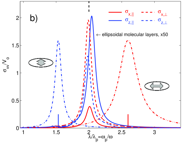
Figure 1: a) A cut through a coated ellipsoidal nanoparticle. The principal semiaxes perpendicular to the paper are $a_{y}$ and $b_{y}$ respectively. The relevant dielectric functions $\epsilon_{in}(\omega)$, $\varepsilon_{c\|}(\omega)$, $\varepsilon_{c\perp}(\omega)$ and $\varepsilon_{m}$ are also indicated. b) Extinction spectrum, where $\sigma_{vv}=\omega\Im[\alpha_{vv}]$, $v=x,y,z$. The dash-dotted curves are for an uncoated metallic ellipsoid, where the red (blue) curve is for the external field along the $x$-axis ($z$-axis). The red solid ($x$-direction) and blue solid ($z$-direction) curves correspond to the case of an ellipsoidal molecular layer (without an interior metallic region, i.e. we set $\epsilon_{i}=1$) with a resonance parallel to the layer normal. Here, this situation is modeled by taking $\gamma_{0\|}/v_{0}=0.2$, $\gamma_{\infty\|}/v_{0}=0.02$, and $\gamma_{0\perp}/v_{0}=\gamma_{\infty\perp}/v_{0}=0.01$ (corresponding to effective oscillator strength $c_{0\|}\approx 2.26$, and large frequency refractive index ${\rm n}_{\|}\approx 1.06$, see text). The red dashed ($x$-direction) and blue dashed ($z$-direction) curves are for the case that the molecular layer has a resonance perpendicular to the layer normal. We take $\gamma_{0\perp}/v_{0}=0.1$ and $\gamma_{\infty\perp}/v_{0}=\gamma_{0\|}/v_{0}=\gamma_{\infty\|}/v_{0}=0.01$ (so that $c_{0\perp}\approx 1.13$ and ${\rm n}_{\perp}\approx 1.07$). The following parameters were used: $e_{o}^{2}=0.8$, $s=1$, $\Delta_{V}=0.08$, $\Gamma_{p}/\omega_{p}=0.05$, $\omega_{0\|}/\omega_{p}=\omega_{0\perp}/\omega_{p}=0.5$, $\Gamma_{\|}/\omega_{p}=\Gamma_{\perp}/\omega_{p}=0.03$ and $\varepsilon_{m}=1$. The extinction cross-sections are shown in units of the total volume $V_{o}$. The solid and dashed vertical bars indicate the plasmon and molecular resonance frequencies, respectively. Notice the small peak heights of the molecular layer resonances (here enlarged by a factor 50) compared with the plasmon resonance heights.

The full expression for the dipolar polarizability $\alpha_{vv}$ (defined through $p_{v}=4\pi\varepsilon_{0}\varepsilon_{m}\alpha_{vv}E_{0v}$, where $p_{v}$ is the $v$-component, $v=x,y$ or $z$, of the induced dipole moment and $\varepsilon_{0}$ is the permittivity of free space) in terms of the geometric and dielectric entities above is given in Refs. Ambjornsson_Mukhopadhyay, and Ambjornsson_Apell_Mukhopadhyay, : A knowledge of $\alpha_{vv}$ requires a function $H_{v}(u,s;q)$, satisfying Heun’s equation Ronveaux ; Slavyanov_Lay , evaluated at the inner, $q=e_{i}^{2}$, and the outer, $q=e_{o}^{2}$, surfaces. The shape parameter $s$ was introduced above. The anisotropy in the dielectric function of the coating ($\varepsilon_{c\|}$ and $\varepsilon_{c\perp}$) enters through $u$ defined as

$$u=u_{\pm}=-\frac{1}{2}\pm\frac{1}{2}(1+8\varepsilon_{\perp}\varepsilon_{\parallel}^{-1})^{1/2},$$ (1)

where $\varepsilon_{\mu}(\omega)=\varepsilon_{c\mu}(\omega)/\varepsilon_{m}$ ($\mu=\perp$ or $\|$). For the case of spheroids (two of the principal axes are equal) $H_{v}(u,s;q)$ is expressible in terms of hypergeometric functions, which are available in standard mathematical numerical packages, such as MatLab or Mathematica. For general ellipsoids $H_{v}(u,s;q)$ is straightforwardly generated using a recurrence relation, explicitly given in Ref. Ambjornsson_Mukhopadhyay, . Introducing a second function $r_{v}(u,s;q)$ ($v$=$x$, $y$ or $z$), required while implementing the boundary conditions and defined in terms of $H_{v}(u,s;q)$ according to

$$r_{v}(u,s;q)=1-f_{v}(s;q)\{1-u+2q\frac{\partial}{\partial q}\ln{[}H_{v}(u,s;q){]}\},$$ (2)

where $f_{x}(s;q)=1$, $f_{y}(s;q)=1-sq$ and $f_{z}(s;q)=1-q$, the polarizability of an ellipsoid with an anisotropic coating is

$$\alpha_{vv}=\frac{V_{o}}{4\pi n_{v}^{o}}\frac{I_{v}(\kappa=-1)}{I_{v}(\kappa=1/n_{v}^{o}-1)},$$ (3)

where

$$I_{v}(\kappa) = {[}r^{o}_{v}(u_{+})+\kappa\varepsilon_{\parallel}^{-1}{]}{[}r^{i}_{v}(u_{-})-\varepsilon_{i}\varepsilon_{\parallel}^{-1}{]}$$ (4)

$$-\rho_{v}{[}r^{o}_{v}(u_{-})+\kappa\varepsilon_{\parallel}^{-1}{]}{[}r^{i}_{v}(u_{+})-\varepsilon_{i}\varepsilon_{\parallel}^{-1}{]}.$$

where $\varepsilon_{i}=\varepsilon_{\rm in}/\varepsilon_{m}$, and we have above introduced the short-hand notation $r_{v}^{i}(u_{\pm})\equiv r_{v}(u_{\pm},s;e_{i}^{2})$ and $r_{v}^{o}(u_{\pm})\equiv r_{v}(u_{\pm},s;e_{o}^{2})$. $n^{o}_{v}$ is the standard depolarization factor for the $v$-direction for the outer surface and satisfies the sum ruleLandau_Lifshitz_ecm ; Ambjornsson_Mukhopadhyay ; Ambjornsson_Apell_Mukhopadhyay : $n_{x}^{o}+n_{y}^{o}+n_{z}^{o}=1$. We have also introduced

$$\rho_{v}\equiv(\frac{e_{o}}{e_{i}})^{(u_{+}-u_{-})}\frac{H_{v}^{o}(u_{-})H_{v}^{i}(u_{+})}{H_{v}^{o}(u_{+})H_{v}^{i}(u_{-})},$$ (5)

where $H_{v}^{o}(u_{\pm})\equiv H_{v}(u_{\pm},s;e_{o}^{2})$ and $H_{v}^{i}(u_{\pm})\equiv H_{v}(u_{\pm},s;e_{i}^{2})$. We note that the total volume $V_{o}$ only enters as a prefactor in the expression for $\alpha_{vv}$. The geometry of the particle enters through the geometric entities $n_{v}^{o}$, $r_{v}^{i}(u_{\pm})$ and $r_{v}^{o}(u_{\pm})$. The standard isotropic depolarization factor $n_{v}^{o}$ depends only on the shape ($s$ and $e_{o}^{2}$), whereas $r_{v}^{i}(u_{\pm})$ and $r_{v}^{o}(u_{\pm})$ couple the geometry to the dielectric asymmetry of the coating. For an anisotropic coated sphere the expression for the polarizability agrees with the result obtained in Ref. Lucas_Henrard_Lambin, . For an isotropic coating $\varepsilon_{\|}=\varepsilon_{\perp}$ the polarizability reduces to the standard result given in for instance Ref. Bohren_Huffman, . The imaginary part of $\alpha_{vv}$ is directly accessible through experimental extinction or absorption measurements. Explicitly, the extinction cross-section is $\sigma_{vv}=\omega\Im[\alpha_{vv}]$, where $\Im[\cdot]$ denotes the imaginary part of the entity within the square brackets []. In order to obtain the response of the coated metallic nanoparticle we must proceed by incorporating realistic microscopic dielectric functions for the coating and metal into the expression (3) for the dipolar particle polarizability.

Let us consider the interior metallic region. In a standard fashion we assume that the dielectric function of the metal is described by a Drude function:

$$\varepsilon_{\rm in}(\omega)=\varepsilon_{\infty}-\frac{\omega_{p}^{2}}{\omega(\omega+i\Gamma_{p})}$$ (6)

with $\omega_{p}$ being the plasmon frequency, $\Gamma_{p}$ is a phenomenological damping parameter and $\varepsilon_{\infty}$ is the dielectric function for large frequencies. We take $\varepsilon_{\infty}=1$ throughout this study. An uncoated metallic ellipsoidal particle in vacuum ($\epsilon_{m}=1$) has dipolar plasmon resonance frequencies

$$\omega_{pv}=\omega_{p}\sqrt{n_{v}^{i}},$$ (7)

where $n_{v}^{i}$ is the (purely geometric) depolarization factor of the inner ellipsoidal surface Bohren_Huffman ; Landau_Lifshitz_ecm ; Ambjornsson_Mukhopadhyay (see also appendix A).

We now give the dielectric function of the coating; we assume that the coating consists of molecules with dipolar polarizabilities which are diagonal but with different components in normal and tangential directions; we denote the polarizabilities by $\gamma_{\|}$ ($\gamma_{\perp}$), [where a subscript $\perp$ ($\|$) denotes polarizability component perpendicular (parallel) to the metallic surface normal]. Let us relate $\gamma_{\|}$ and $\gamma_{\perp}$ to the dielectric functions $\varepsilon_{{\rm c}\parallel}(\omega)$ and $\varepsilon_{{\rm c}\perp}(\omega)$ appearing in coated ellipsoid polarizability $\alpha_{vv}$: assuming that the surface is locally flat, and imposing the conditions that the normal component of the total macroscopic electric field and the tangential component of the displacements field are continuous across the surface separating the molecular coating from the surrounding, we straightforwardly arrive at the following relation between the molecular polarizabilities and the coating dielectric functions Bagchi_Barrera_Fuchs

$$\varepsilon_{\perp}(\omega) = 1+\frac{4\pi\gamma_{\perp}(\omega)}{v_{0}},$$

$$\varepsilon_{\|}(\omega)^{-1} = 1-\frac{4\pi\gamma_{\|}(\omega)}{v_{0}},$$ (8)

where $v_{0}$ is the unit cell volume per molecule.Ambjornsson_Apell_Mukhopadhyay Explicitly, we take the following form for the renormalized molecular polarizabilities

$$\gamma_{\mu}(\omega)=\gamma_{\infty\mu}+(\gamma_{0\mu}-\gamma_{\infty\mu})\frac{\omega_{0\mu}^{2}}{\omega_{0\mu}^{2}-\omega^{2}-i\omega\Gamma_{\mu}}$$ (9)

where $\gamma_{0\mu}$ is the static polarizability of the molecules, $\gamma_{\infty\mu}$ is the high frequency polarizability, $\omega_{0\mu}$ is a resonance frequency and $\Gamma_{\mu}$ is a damping parameter.Ambjornsson_Apell ; Bagchi_Barrera_Fuchs It is sometimes convenient to characterize the electromagnetic response properties of the coating by the effective oscillator strength (compare to Ref. Wiederrecht_Wurtz_etal, ) $c_{0\mu}=4\pi(\gamma_{0\mu}-\gamma_{\infty\mu})/v_{0}$, and the large frequency refractive indices ${\rm n}_{\perp}={\varepsilon_{c\perp}(\omega=\infty)}^{1/2}=(1+4\pi\gamma_{\infty\mu}/v_{0})^{1/2}$ and ${\rm n}_{\|}={\varepsilon_{c\|}(\omega=\infty)}^{1/2}=(1-4\pi\gamma_{\infty\mu}/v_{0})^{-1/2}$. We point out that the induced dipole coupling between molecules (and image dipoles in the metal) in general, introduce extra anisotropy by renormalizing the resonance frequencies, static polarizabilities, large frequency polarizabilities and damping parameters compared to their “bare” values, Bagchi_Barrera_Fuchs ; Ambjornsson_Apell ; Ambjornsson_Apell_Mukhopadhyay and all such anisotropies are included in the expression (9).

To summarize, the general procedure for obtaining the polarizability $\alpha_{vv}(\omega)$ ($v=x,y,z$) for an ellipsoidal metallic nanoparticle coated with an anisotropic molecular layer is: Consider a nanoparticle with principal semiaxes $a_{x}$, $a_{y}$, and $a_{z}$. The size of the molecules together with these nanoparticle principal semiaxes determine the outer principal semiaxes $b_{x}$, $b_{y}$ and $b_{z}$, see Fig. 1. From these six principal semiaxes one calculates the the total volume $V_{o}$, and the shape parameters $s$, $e_{i}^{2}$, $e_{o}^{2}$ (for small coating thickness $e_{i}^{2}$ and $e_{o}^{2}$ are related through the relative coating thickness $\Delta_{V}$). The problem is completed by specifying the metallic nanoparticle parameters in Eq. (6), and the renormalized polarizability parameters of Eq. (9); alternatively, one may use experimental results for the nanoparticle and coating dielectric functions. Finally, the parameters above are used in the expression for $\alpha_{vv}(\omega)$ explicitly given in Eq. (3).

For the case where the coating resonance frequency $\omega_{0\mu}$ is close to being degenerate with one of the particle plasmon resonances (i.e., $\omega_{pv}$ of Eq. (7)) one expect hybridization between the two resonances.HalasScience In order to address this point we proceed by finding an approximate expression for the resonance frequencies for $\alpha_{vv}(\omega)$. Assuming a thin coating $\Delta_{V}\ll 1$, and utilizing the near resonance approximation (the large $u$-result Ambjornsson_Mukhopadhyay ; Ambjornsson_Apell_Mukhopadhyay ) we obtain a simplified form for $\alpha_{vv}$, as detailed in appendix A. Below we use this $\alpha_{vv}$ for obtaining approximate expressions for the coupled (hybridized) resonance frequencies and for the extinction peak height at these resonances. The damping constants associated with the hybridized resonances are given in Eq. (46). We point out the the approximate expressions for $\alpha_{vv}$ given in appendix A are useful for investigating other quantities as well.

The resonance frequencies are obtained by finding the poles of $\alpha_{vv}$; using the results in the appendix we find that resonances occur at frequencies $\omega=\omega_{v\mu}^{\pm}$ given by (see Eqs. (30) (31), (36) and (37))

$$(\omega_{v\mu}^{\pm})^{2}=\omega_{a\mu}^{2}\pm\left(\omega_{d\mu}^{4}+\omega_{0\mu}^{4}D_{v\mu}^{2}\right)^{1/2},$$ (10)

where for brevity, we have introduced the notations $\omega_{a\mu}^{2}=[(\omega^{o}_{pv})^{2}+\omega_{0\mu}^{2}]/2$ and $\omega_{d\mu}^{2}=[(\omega^{o}_{pv})^{2}-\omega_{0\mu}^{2}]/2$, with $\omega^{o}_{pv}=\omega_{p}\sqrt{n_{v}^{o}}$; we have also introduced above a (dimensionless) parallel coupling strength

$$D_{v\|}=\left[\Delta_{V}g_{v\|}c_{0\|}(1-n_{v}^{o})\frac{\omega_{p}^{2}-\omega_{a\|}^{2}}{\omega_{0\|}^{2}}\right]^{1/2},$$ (11)

and a perpendicular coupling strength

$$D_{v\perp}=\left[\Delta_{V}g_{v\perp}c_{0\perp}n_{v}^{o}\frac{\omega_{a\perp}^{2}}{\omega_{0\perp}^{2}}\right]^{1/2}.$$ (12)

with the effective oscillator strength $c_{0\mu}=4\pi(\gamma_{0\mu}-\gamma_{\infty\mu})/v_{0}$ as defined before, and the geometric factors defined as

$$g_{v\perp}=1-\frac{1}{F_{o}f_{v}^{o}},\quad{\rm and}\quad g_{v\|}=\frac{1}{F_{o}f_{v}^{o}}.$$ (13)

where $f_{v}^{o}=f_{v}(s;e_{o}^{2})$ so that, $f_{x}^{o}=1$, $f_{y}^{o}=1-se_{o}^{2}$, $f_{z}^{o}=1-e_{o}^{2}$ and $F_{o}=1+(1-se_{o}^{2})^{-1}+(1-e_{o}^{2})^{-1}$. The quantities $g_{v\mu}$ appear also in the polarizability for an anisotropic shell Ambjornsson_Apell_Mukhopadhyay and satisfies the three sum rules $g_{x\|}+g_{y\|}+g_{z\|}=1$, $g_{x\perp}+g_{y\perp}+g_{z\perp}=2$ and $g_{v\perp}+g_{v\|}=1$. Eq. (10) has the same form as that for two dipole coupled oscillators, see for instance Ref. Pippard, (also compare with Ref. HalasScience, ). The strength of the molecular-plasmon interaction is characterized by the polarization and molecular orientation dependent coupling strength $D_{v\mu}$, which depend on the relative coating volume parameter $\Delta_{V}$, on the molecular response properties through $c_{0\mu}$, as well as on different geometric quantities.

For a sphere ($e_{o}^{2}\rightarrow 0$) we have that $g_{v\|}=1/3$, $g_{v\perp}=2/3$, and $n_{v}^{o}=1/3$ and Eqs. (11) and (12) become

$$D_{v\|}|_{\rm sph} = \left[\Delta_{V}\frac{c_{0\|}}{27}\left(5\frac{\omega_{p}^{2}}{\omega_{0\|}^{2}}-3\right)\right]^{1/2},$$

$$D_{v\perp}|_{\rm sph} = \left[\Delta_{V}\frac{c_{0\perp}}{27}\left(\frac{\omega_{p}^{2}}{\omega_{0\perp}^{2}}+3\right)\right]^{1/2}.$$ (14)

The equations above quantify the degree of hybridization and its dependence on molecular orientation for a coated metallic sphere. cylindrical_case

We notice from Eq. (10) that if the coating and particle plasmon resonance frequencies are well separated, in the sense $D_{v\mu}^{2}\ll\omega_{d\mu}^{4}/\omega_{0\mu}^{4}$, then the resonance frequencies are the uncoupled ones: $\omega_{pv}$ and $\omega_{0\mu}$.

In contrast, for $D_{v\mu}^{2}\gg\omega_{d\mu}^{4}/\omega_{0\mu}^{4}$, we have resonances approximately at

$$\omega_{v\mu}^{\pm}\approx\omega^{o}_{pv}(1\pm D_{v\mu})^{1/2}\quad{\rm for}\quad\omega^{o}_{pv}=\omega_{0\mu},$$ (15)

and

$$D_{v\|} \approx (1-n_{v}^{o})(\Delta_{V}g_{v\|}c_{0\|}/n_{v}^{o})^{1/2},$$

$$D_{v\perp} \approx (\Delta_{V}g_{v\perp}c_{0\perp}n_{v}^{o})^{1/2}.$$ (16)

Thus, for $\omega^{o}_{pv}\approx\omega_{0\mu}$, we get $D_{v\mu}\propto\sqrt{\Delta_{V}}$ and we have strong hybridization between the nanoparticle and coating resonance frequencies, as will be illustrated in more detail in the next section. We also notice from Eq. (16) that for small $n_{v}^{o}$, $D_{v\|}$ can be substantially larger than $D_{v\perp}$, which can give a wider separation between $\omega_{v\|}^{+}$ and $\omega_{v\|}^{-}$ compared with that for $\omega_{v\perp}^{\pm}$.

The extinction peak height at one of the resonance frequency $\omega_{v\mu}^{\pm}$ is $\sigma_{vv}(\omega=\omega_{v\mu}^{\pm})$; using Eq. (25) we convert this quantity into a scaled peak height $T^{\pm}_{v\mu}=4\pi\sigma_{vv}(\omega^{\pm}_{v\mu})/(V_{o}(\omega^{\pm}_{v\mu})^{2})$ at the resonances. Employing the thin coating approximation and assuming that we are close to a resonance Eqs. (32) and (38) apply, i.e. we have the approximate result

$$T^{\pm}_{v\mu} = \frac{\omega_{p}^{2}}{(\omega_{v\mu}^{\pm})^{2}}$$ (17)

$$\times\frac{\big{(}\omega_{0\mu}^{2}-(\omega_{v\mu}^{\pm}\big{)}^{2})}{\Gamma_{p}\big{(}\omega_{0\mu}^{2}-(\omega_{v\mu}^{\pm})^{2}\big{)}+\Gamma_{\mu}\big{(}(\omega^{o}_{pv})^{2}-(\omega_{v\mu}^{\pm})^{2}\big{)}},$$

which for $\omega^{o}_{pv}\approx\omega_{0\mu}$ gives

$$T^{\pm}_{v\mu}=\frac{1}{n_{v}^{o}(\Gamma_{p}+\Gamma_{\mu})}\,\frac{1}{1\pm D_{v\mu}},$$ (18)

with $D_{v\mu}$ given by Eq. (16).

For the case of an uncoated metallic nanoparticle the scaled peak height takes the form $T_{vp}=1/(n_{v}^{o}\Gamma_{p})$ (see Eq. (26)). Eq. (18) shows that at strong coupling (i.e. for $\omega^{o}_{pv}\approx\omega_{0\mu}$), $T^{\pm}_{v\mu}$ are of the same order of magnitude as $T_{vp}$.

For a very thin coating without any interior metal we have: $T_{v\mu}(\varepsilon_{i}=1)\approx\Delta_{V}g_{v\mu}c_{0\mu}/\Gamma_{\mu}$ (see Eqs. (29) and (35), and Ref. Ambjornsson_Apell_Mukhopadhyay, ), which is much smaller than $T_{vp}$. Comparing with Eq. (17) we notice that $T^{\pm}_{v\mu}/T_{v\mu}(\varepsilon_{i}=1)\propto(\Delta_{V})^{-1}$ (note however that $\omega_{v\mu}^{\pm}$ depends on $\Delta_{V}$ ), revealing substantial surface enhancement (see next section).

III Results and Discussions.

In the following, we illustrate the electromagnetic response properties of a coated metallic nanoparticle via the extinction cross-section $\sigma_{vv}=\omega\Im[\alpha_{vv}]$ for the case of a prolate ($a_{y}=a_{z}$, i.e. $s=1$, “cigar-shaped”) spheroid. We consider two different situations: the case when the molecules in the coating have their “resonant” axes (i) parallel and (ii) perpendicular to the surface normal. The polarizability component along the resonant axis is $\alpha_{\|}$ in case (i) and $\alpha_{\perp}=\alpha_{\|}/2$ in case (ii), which corresponds to coatings with identical but differently oriented molecules. For each of the two cases, the external field $\vec{E}_{0}$ is applied either along the long axis ($x$-axis) or the short axis ($y$- or $z$-axis).

In Fig. 1b, the polarization averaged extinction cross-section for an uncoated metallic spheroid is shown together with the cross-section for an spheroidally shaped molecular layer without an interior nanoparticle and with the resonant transition dipole moments oriented in the parallel and perpendicular directions. There are two plasmon peaks, as expected for a spheroidal metal particle (two of the principal axes equal), with resonance wavelengths to the red ($\vec{E}_{0}\|x$-axis) and to the blue ($\vec{E}_{0}\|y,z$-axes) of the familiar LSP resonance of a sphere ($\lambda/\lambda_{p}=\sqrt{3}\approx 1.73$). The extinction peaks of the molecular layer is about 50 times weaker than the plasmons for both molecular orientations. Notice that, for geometric reasons, the extinction peak height for the molecular layer is smallest for the case where the external field is in the $x$-direction, with the molecules oriented in the parallel direction; see Ref. Ambjornsson_Apell_Mukhopadhyay, for a thorough discussion on geometric and molecular orientation dependent effects in the response of an ellipsoidal molecular layer. Also notice the small difference in peak position between case (i) and (ii); in Ref. Ambjornsson_Apell_Mukhopadhyay, it was shown that for $\Delta_{V}\ll 1$ there are no curvature induced shifts for the molecular layer resonance frequencies (see also appendix A). Here, $\Delta_{V}$ is not sufficiently small and there are some minor shifts of the resonance frequencies.

In Fig. 2, we show extinction spectra corresponding to the full coated spheroid response problem for the four distinct cases mentioned above, i.e molecular orientation perpendicular (a, b) or parallel (c, d) to the surface normal and incident field parallel to the short (a, c) or the long (b, d) spheroid axes. The different colors of the curves corresponds to different coating resonance frequencies $\omega_{0\mu}$. It is clear that there is strong hybridization between the coating and plasmon resonances whenever $\omega_{0\mu}\approx\omega_{pv}$ ($\mu=\|,\perp$ and $v=x,y,z$) in all cases. However, the degree of hybridization differs greatly between the different molecular orientations and polarization configurations.

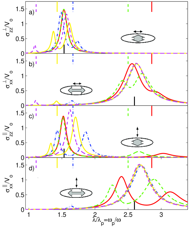
Figure 2: Extinction spectrum for a prolate coated spheroid with different orientations of the molecules on the surface. The spectrum is in units of the total volume $V_{o}$ of the coated spheroid. $\sigma^{\mu}_{vv}=\omega\Im[\alpha_{vv}]$, ($\mu=\|,\perp$ and $v=x,z$) and $\lambda=2\pi c/\omega$ is the wavelength of the external electromagnetic field. a) The external field is along the $z$-axis (short axis) of the spheroid. The molecules have their resonant axes perpendicular to the metallic particle normal; b) the external field along the $x$-axis (long axis), and the molecules are perpendicular to the layer normal; c) the field is along the $z$-axis, and the molecules have their resonant axis parallel to the layer normal; d) the field is along the $x$-axis, and the molecules are oriented parallel to the layer normal. The different colors are spectrum for different molecular resonant wavelengths; the upper vertical bars indicate these resonance wavelengths $\lambda_{0\mu}=2\pi c/\omega_{0\mu}$. Here, we chose the following values for $\omega_{0\mu}$: $0.35\omega_{p}$, $0.4\omega_{p}$, $0.6\omega_{p}$, $0.7\omega_{p}$, $0.9\omega_{p}$. The lower vertical bar is the particle plasmon resonance wavelengths $\lambda_{pv}=2\pi c/\omega_{pv}$ ($v=x,z$). The same parameters as in Fig. 1 were used. Notice the strong hybridization when $\lambda_{0\mu}\approx\lambda_{pv}$ and increased peak height (surface enhanced absorption) for the molecular resonance, compared with Fig. 1b.

In order to investigate the peak height of the resonances (see Fig. 2) Fig. 3 show the scaled peak height $T^{\pm}_{v\mu}$ (defined in Eq. (25)) compared to the scaled peak height $T_{v\mu}(\varepsilon_{i}=1)$ for a molecular layer (obtained from Fig. 1), for different coating resonance frequencies. A comparison to the result given in Eq. (17) is also made. We notice the two coupled resonances obtain similar peak height as $\omega_{0\mu}$ approaches the particle plasmon frequency $\omega_{pv}$. We also point out that the approximate expression Eq. (17) works surprisingly well, considering that it is based on a close to resonance and thin coating approximation, even far off the resonances.

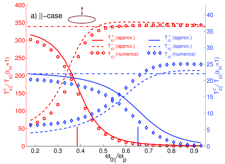
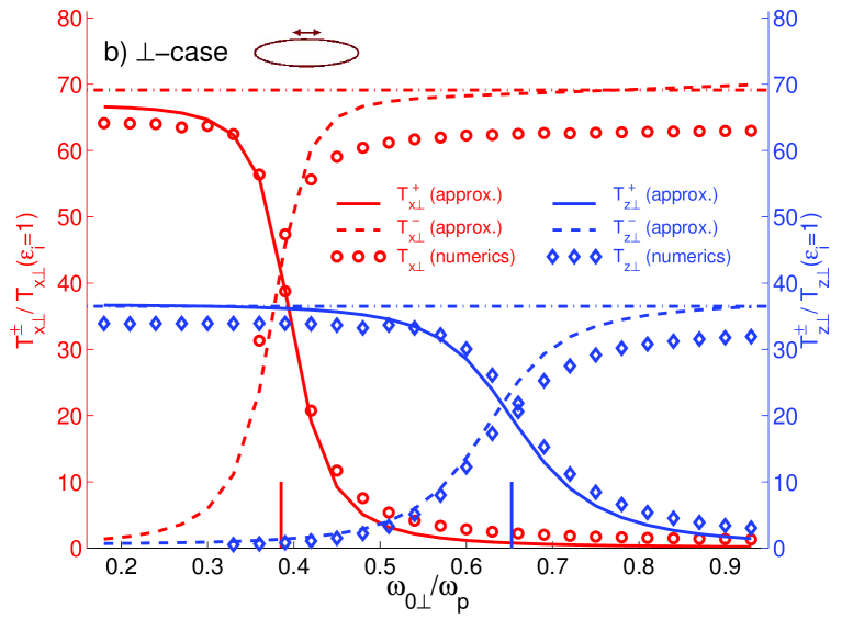
Figure 3: Scaled peak height for the coupled resonances in a coated prolate metal spheroid for the case a) when the coating molecules have their resonant axis parallel to the surface normal and b) for a perpendicular resonance. The resonance frequencies $\omega^{\pm}_{v\mu}$ of the extinction (see Figs. 2 and 4) for different $\omega_{0\mu}$ was numerically determined and used to calculate the scaled peak height $T^{\pm}_{v\mu}=4\pi\sigma_{vv}(\omega^{\pm}_{v\mu})/(V_{o}(\omega^{\pm}_{v\mu})^{2})$ ($v=x,z$ and $\mu=\|,\perp$), see Eq. (25). The peak heights were normalized by the molecular layer peak heights $T_{v\mu}(\varepsilon_{i}=1)$ obtained from Fig. 1. The vertical solid lines correspond to the two plasmon resonances, $\omega_{px}$ and $\omega_{pz}$, Eq. (7). The dashdotted horizontal lines correspond to the plasmon peak heights as given in the text right after Eq. (17). The solid and dashed curves are the approximate results given in Eq. (17). The same parameters as in Fig. 1 were used. Notice the different ranges of the ordinates, and that the abscissas are in frequency units.

When the molecular resonance is far above or far below a plasmon resonance, we have a situation that can best be described as surface-enhanced absorption from the molecular layer Moskovits1985 , i.e the magnitude of the molecular resonance peak is greatly enhanced but its position and width is not changed dramatically from the case of a ”free” molecular layer, see Figs 2 and 3. In this regime, the particle plasmons (at $\lambda_{pv}$, with $v=x,y,z$) become either red-shifted or blue-shifted relative to the uncoated metallic spheroid resonance wavelength depending on the molecular resonance wavelength $\lambda_{0}$. Interestingly, the enhanced absorption from the molecular layer is not symmetric on the two sides of the plasmon. This can be seen when comparing Fig. 2 a) and c) (see also Fig. 3), corresponding to polarization along the short axis of the spheroid. When the molecular resonance is far to the red of the plasmon, absorption enhancement is seen for the case when the molecular resonance axis is parallel to the surface normal (Fig. 2 c), but not for the perpendicular case (Fig. 2 a). The situation is reversed (although less pronounced) when the molecular resonance is to the blue of the plasmon, i.e absorption enhancement occurs for the perpendicular but not for the parallel case. Similar effects are seen in Fig. 2 b) and d), corresponding to polarization along the long axis. From Fig. 3a) we notice that particularly strong surface enhancement (roughly a factor 50 for the extinction cross section for the parameters used here) occur to the red of the plasmon for the parallel case with the incident field along the x-axis.

The differences above can be understood as follows: To the red of a plasmon resonance, the induced field from the particle is in phase with the applied field and normal to the surface at the poles of the particle (where the poles are defined by the direction of the induced dipole), resulting in enhanced absorption from molecules oriented parallel the surface normal. Molecules with the perpendicular orientation instead couple mainly to the total field around the equator of the particle, where the field is perpendicular to the surface normal. But to the red this field is weak, because here the induced field is out-of-phase with the applied field. Hence, there is very little enhanced absorption to the red of the plasmon in Fig 2 a) but a large enhancement in Fig. 2 c). The same type of arguments apply to the case when the molecular resonance is to the blue of the plasmon, but here the situation becomes reversed because the induced particle dipole is out-of-phase with the incident field.Kottman

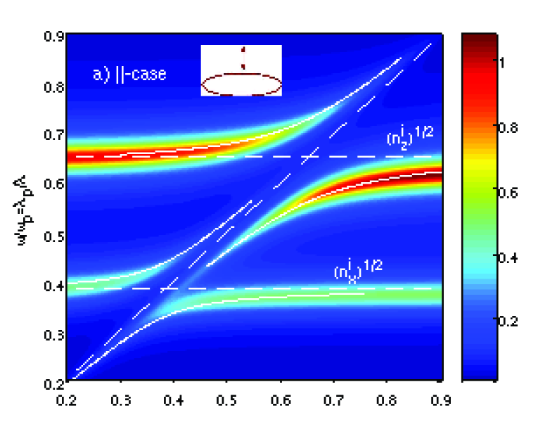
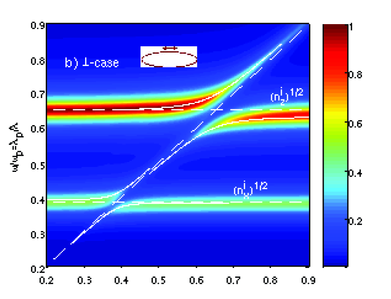
Figure 4: Illustration of strong coupling and ”avoided crossing” between the plasmonic and molecular resonances of a coated prolate metal spheroid for the case a) when the molecules have their resonant axis parallel to the surface normal and b) for a perpendicular resonance. The horizontal dashed lines correspond to the two plasmon resonances, $\omega_{px}$ and $\omega_{pz}$, and the diagonal dashed lines denotes $\omega=\omega_{0\mu}$. The solid white curves are the approximate results for the coupled resonances as given in Eq. (10). The same parameters as in Fig. 1 were used. Notice that the axes are in frequency units.

The case when the molecular resonance is degenerate with one of the plasmons corresponds to a regime that can not be described in terms of enhanced absorption. Instead, we have two completely hybridized resonances that exhibit ”avoided crossing”, analogous to the case of two strongly coupled (quantum or classical) harmonic oscillators, as is seen in Eq. (10). Fig. 4 illustrates this behavior for the two molecular orientations considered. In the vocabulary of Ref. HalasScience, , the high frequency modes $\omega_{v\mu}^{+}$ in Eq. (10) correspond to ”anti-bonding” combinations, i.e. the case where the induced dipole on the particle is out-of-phase with the molecular transition dipoles, while the ”bonding” modes $\omega_{v\mu}^{-}$ corresponds to the case when the excitations are in phase. In a diabatic representation, this corresponds to Rabi oscillations in which the excitation energy oscillates back and forth between the plasmonic particle and the molecular layer. As can be seen in Fig. 4, the mode splitting is much more significant when the molecular resonance is oriented parallel to the surface normal (Fig. 4a) than for the perpendicular case (Fig. 4b). This difference simply reflects the predominant polarization of the local field at the surface (the field would be strictly parallel to the surface normal for a perfect conductor at zero frequency). We also note that the splitting (expressed in frequency units) is larger for the plasmon that corresponds to polarization along the short axis of the prolate spheroid for both molecular orientations, which is somewhat surprising considering that the field enhancement is highest at the sharp ends of the spheroid. Kottman However, the coupling strength is determined by the surface integrated local field at the two plasmon resonance frequencies, and for geometric reasons this quantity is higher for the doubly-degenerate short-axis plasmon in the present case.

To the best of our knowledge, there are no experimental studies that have directly probed the orientation dependent plasmon-molecule coupling discussed here. However, the advanced nanofabrication and molecular functionalization technologies of today clearly make such studies a realistic possibility. One of the most interesting options could be to use a plasmonic nanoparticle covered by an ordered layer of chromophores as a nanoscopic bio/chemo sensor. For example, it can be expected that the exact orientation of the chromophores on the surface will be sensitive to pH and to the interaction with molecules in solution. The chromophores might also be incorporated as functional groups into larger biomacromolecules that change orientation/conformation upon biorecognition reaction with an analyte. Such sensing reactions would then affect the coupling between the surface plasmons and the chromophores, giving rice to pronounced changes in the extinction or scattering spectrum of the composite nanoparticle. To illustrate this possibility, Fig. 5 shows the difference spectra between the parallel and perpendicular orientations discussed above. As expected, the difference is largest for molecular resonance wavelengths that overlap the LSP modes. However, a noticeable difference is observed even far off the plasmon resonances, indicating that molecular orientation effects needs to be taken into account also in classical nanoparticle refractive index sensing experiments.

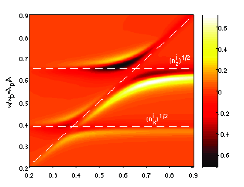
Figure 5: Difference in averaged extinction cross-section $\Delta\sigma/V_{o}=(\sigma^{\|}-\sigma^{\perp})/V_{o}$ (indicated by the different colors) between the parallel and perpendicular cases as shown in Fig. 4 a) and b), as a function molecular resonance frequency $\omega_{0}=\omega_{0\|}=\omega_{0\perp}$ and external field frequency $\omega$. Note that the axes are in frequency units.

IV Summary

We have described an analytic method for calculating the optical response of arbitrary ellipsoidal nanoparticles with anisotropic molecular coatings in the small particle limit and applied this theory to the case of a prolate metal spheroid covered with chromophores. The results show that the hybridization between the molecular resonance and the localized plasmon resonances of the nanoparticle is highly anisotropic. It is suggested that this sensitivity can be utilized for novel bio/chemo sensing applications that are based on molecular orientation rather than refractive index contrast.

Appendix A Approximate expression for coupled resonances and peak heights and widths

In this appendix we use the large $u$ (close to a resonance) and thin coating approximations for the coated ellipsoid polarizability given in Eq. (3) in order to derive approximate expressions for the coupled resonance frequencies as well as for the peak heights and widths of these excitations.

Close to a resonance ($u$ large) and for a thin coating ($\Delta_{V}\ll 1$) we have that Eq. (3) becomes

$$\alpha_{vv}=\frac{V_{o}}{4\pi n_{v}^{o}}\frac{J_{v}(\kappa=-1)}{J_{v}(\kappa=1/n_{v}^{o}-1)},$$ (19)

with

$$J_{v}(\kappa)=\varepsilon_{i}+\kappa+\Delta_{V}g_{v\perp}\varepsilon_{\perp}+\Delta_{V}\varepsilon_{i}g_{v\|}\varepsilon^{-1}_{\|}\kappa$$ (20)

in an identical fashion as the derivation given in Ref. Ambjornsson_Apell_Mukhopadhyay, . The geometric factors $g_{v\|}$ and $g_{v\perp}$ ($v=x,y,z$) are given in Eq. (13). Explicit expressions for the dielectric functions $\varepsilon_{i}$, $\varepsilon_{\perp}$ and $\varepsilon_{\|}$ appearing in Eq. (20) are given in Eqs. (6) and (8). Below we investigate $J_{v}(\kappa)$ in the limits of (1.) no coating $\Delta_{V}=0$; (2.) external field frequency close to the parallel resonance frequency, $\omega\approx\omega_{0\|}$; (3.) external field frequency close to the perpendicular resonance frequency, $\omega\approx\omega_{0\perp}$. In (4.) we derive expressions for the peak widths of the hybridized resonances.

A.1 No coating, $\Delta_{V}=0$

For the case of no coating, $\Delta_{V}=0$, we have that $J_{v}(\kappa)=\varepsilon_{i}+\kappa$ and therefore the polarizability, Eq. (19), can be written

$$\alpha_{vv}(\omega)=\frac{V_{o}}{4\pi n_{v}^{o}}\frac{K_{v}(\kappa=-1)}{K_{v}(\kappa=1/n_{v}^{o}-1)},$$ (21)

where $K_{v}$ equals $J_{v}$ multiplied a by a factor independent of $\kappa$, and explicitly,

$$\Re[K_{v}(\kappa)] = \omega_{p}^{2}-\omega^{2}(1+\kappa),$$

$$\Im[K_{v}(\kappa)] = -\omega\Gamma_{p}(1+\kappa),$$ (22)

with $\Re[\cdot]$ ($\Im[\cdot]$) denoting the real (imaginary) part of the entity inside []. The resonance criterion $\Re[K_{v}(\kappa=1/n_{v}^{o}-1)]=0$ gives, together with Eq. (22), the uncoated metallic ellipsoid resonance frequencies:

$$\omega_{{\rm res},v}^{2}=(\omega^{o}_{pv})^{2}=\omega_{p}^{2}n_{v}^{o}$$ (23)

in agreement with Eq. (7) as it should (note that when $\Delta_{V}=0$ then $n_{v}^{i}=n_{v}^{o}$). At one of the resonances the extinction peak height $\sigma_{vv}(\omega_{{\rm res},v})=\omega_{{\rm res},v}\Im[\alpha_{vv}(\omega_{{\rm res},v})]$ is:

$$\sigma_{vv}(\omega_{{\rm res},v}) = -\frac{V_{o}}{4\pi n_{v}^{o}}\frac{\omega\Re[K_{v}(\kappa=-1)]}{\Im[K_{v}(\kappa=1/n_{v}^{o}-1)]}|_{\omega=\omega_{{\rm res},v}}$$ (24)

$$= \frac{V_{o}}{4\pi n_{v}^{o}}\Gamma_{p}^{-1}\omega_{{\rm res},v}^{2},$$

where we have used Eq. (22) and $\omega_{{\rm res},v}$ is given in Eq. (23). It is convenient to define a scaled peak height

$$T_{v}\equiv\frac{4\pi}{V_{o}}\,\frac{\sigma_{vv}(\omega_{{\rm res},v})}{\omega_{{\rm res},v}^{2}},$$ (25)

so that, using Eq. (24), we have

$$T_{v}=T_{vp}=\frac{1}{n_{v}^{o}\Gamma_{p}}.$$ (26)

Thus, for an uncoated nanoparticle $T_{v}$ is a measure of the life time (inverse damping) of the plasmon excitation. We will below use the definition, Eq. (25), to compute approximate scaled peak heights of the coated metallic ellipsoid excitations.

A.2 $\omega\approx\omega_{0\|}$

For the case $\omega\approx\omega_{0\|}$ (and $\omega_{0\|}\neq\omega_{0\perp}$) we neglect the “perpendicular” term in Eq. (20), so that $J_{v}(\kappa)=\varepsilon_{i}+\kappa+\Delta_{V}\varepsilon_{i}g_{v\|}\varepsilon^{-1}_{\|}\kappa$. Using the explicit expressions for the dielectric functions described by Eqs. (6), and (8) along with (9) we find

$$K_{v}(\kappa) = \left[\omega(\omega+i\Gamma_{p})(\omega^{2}-\omega_{0\|}^{2}+i\omega\Gamma_{\|})\right]\times J_{v}(\kappa)$$ (27)

$$\approx (\omega^{2}+i\omega\Gamma_{p}-\omega_{p}^{2})(\omega^{2}-\omega_{0\|}^{2}+i\omega\Gamma_{\|})$$

$$+(\omega^{2}+i\omega\Gamma_{p}-\omega_{p}^{2})\Delta_{V}g_{v\|}c_{0\|}\omega_{0\|}^{2}\kappa$$

$$+(\omega^{2}+i\omega\Gamma_{p})(\omega^{2}-\omega_{0\|}^{2}+i\omega\Gamma_{\|})\kappa,$$

Assuming that $\Delta_{V}\ll 1$, and neglecting terms of order $\Gamma^{2}$ ($\Gamma=\Gamma_{p},\Gamma_{\|}$), and $\Gamma\Delta_{V}$ (the neglected term $\Delta_{V}g_{v\perp}\varepsilon_{\perp}$ is of the same order as the terms neglected here) we find that the polarizability can be written in the same form as in Eq. (21) now with

$$\Re[K_{v}(\kappa)] = (\omega_{0\|}^{2}-\omega^{2})[\omega_{p}^{2}-\omega^{2}(1+\kappa)]$$

$$-\Delta_{V}g_{v\|}c_{0\|}\omega_{0\|}^{2}(\omega_{p}^{2}-\omega^{2})\kappa,$$

$$\Im[K_{v}(\kappa)] = -\omega\Big{(}\Gamma_{p}\big{(}(\omega_{0\|}^{2}-\omega^{2})(1+\kappa)$$ (28)

$$+\Gamma_{\|}\big{(}(\omega_{p}^{2}-\omega^{2}(1+\kappa)\big{)}\Big{)}.$$

We notice that the second term in the expression for $\Re[K_{v}(\kappa)]$ cannot be discarded because the first term may be close to zero. In the limit $\Delta_{V},\Gamma_{\|}\rightarrow 0$ the polarizability reduces to the uncoated result from the previous subsection.

In the limit $\omega_{p},\Gamma_{p}\rightarrow 0$ (i.e. $\varepsilon_{i}=\varepsilon_{\infty}=1$) we recover, to lowest order in $\Delta_{V}$, the result in Ref. Ambjornsson_Apell_Mukhopadhyay, :

$$\alpha_{vv}(\omega)=\Delta_{V}\,\frac{V_{o}}{4\pi}g_{v\|}c_{0\|}\,\frac{\omega_{0\|}^{2}}{\omega_{0\|}^{2}-\omega^{2}-i\omega\Gamma_{\|}}$$ (29)

as it should.

Turning back to the general expression Eq. (28) we find that the resonance condition $\Re[K_{v}(\kappa=1/n_{v}^{o}-1)]=0$ gives resonance frequencies:

$$(\omega_{v\|}^{\pm})^{2} = \frac{\omega_{p}^{2}n_{v}^{o}+\omega_{0\|}^{2}}{2}$$ (30)

$$\pm\left[\Big{(}\frac{\omega_{p}^{2}n_{v}^{o}-\omega_{0\|}^{2}}{2}\Big{)}^{2}+\omega_{0\|}^{4}D_{v\|}^{2}\right]^{1/2}$$

with a dimensionless coupling strength $D_{v\|}$ defined by

$$D_{v\|}^{2}=\Delta_{V}g_{v\|}c_{0\|}(1-n_{v}^{o})\Big{(}\frac{\omega_{p}^{2}}{\omega_{0\|}^{2}}-\frac{\omega_{p}^{2}n_{v}^{o}+\omega_{0\|}^{2}}{2\omega_{0\|}^{2}}\Big{)}.$$ (31)

Using Eq. (25) we find that the scaled peak height $T^{+}_{v\|}$ ($T^{-}_{v\|}$) of the resonance characterized by resonance frequency $\omega_{v\|}^{+}$ ($\omega_{v\|}^{-}$) becomes (for $\omega_{p}\neq 0$)

$$T^{\pm}_{v\|} = \frac{\omega_{p}^{2}}{(\omega_{v\|}^{\pm})^{2}}$$ (32)

$$\times\frac{\big{(}\omega_{0\|}^{2}-(\omega_{v\|}^{\pm})^{2}\big{)}}{\Gamma_{p}\big{(}\omega_{0\|}^{2}-(\omega_{v\|}^{\pm})^{2}\big{)}+\Gamma_{\|}\big{(}\omega_{p}^{2}n_{v}^{o}-(\omega_{v\|}^{\pm})^{2}\big{)}},$$

where we have used the fact that $(\omega_{v\|}^{\pm})^{2}$ is of the order $(\Delta_{V})^{1/2}$, and neglected terms of order $\Delta_{V}$.

We notice from Eq. (30) that if $D_{v\|}\ll|[\omega_{p}^{2}n_{v}^{o}-\omega_{0\|}^{2}]/[2\omega_{0\|}^{2}]|$, then the resonance frequencies are the uncoupled ones: $\omega_{p}\sqrt{n_{v}^{o}}$ and $\omega_{0\|}$.

If instead $D_{v\|}\gg|[\omega_{p}^{2}n_{v}^{o}-\omega_{0\|}^{2}]/[2\omega_{0\|}^{2}]|$, (i.e., for $\omega_{p}^{2}n_{v}^{o}\approx\omega_{0\|}^{2}$), we get $(\omega_{v\|}^{\pm})^{2}\approx\omega_{p}^{2}n_{v}^{o}[1\pm D_{v\|}]$, and

$$T^{\pm}_{v\|}=\frac{1}{n_{v}^{o}(\Gamma_{p}+\Gamma_{\|})}\,\frac{1}{1\pm D_{v\|}}$$ (33)

with $D_{v\|}=(\Delta_{V}g_{v\|}c_{0\|}(1-n_{v}^{o})^{2}/n_{v}^{o})^{1/2}$, showing strong hybridization of the plasmon and coating resonances.

A.3 $\omega\approx\omega_{0\perp}$

For the case $\omega\approx\omega_{0\perp}$ (and $\omega_{0\|}\neq\omega_{0\perp}$) we neglect the “parallel” term in Eq. (20), so that $J_{v}(\kappa)=\varepsilon_{i}++\kappa+\Delta_{V}g_{v\perp}\varepsilon_{\perp}$. Using the explicit expressions for the dielectric functions in Eqs. (6) and (8) along with (9) an identical analysis as in the preceding subsection shows that polarizability can be written in the same form as in Eq. (21) with

$$\Re[K_{v}(\kappa)] = (\omega_{0\perp}^{2}-\omega^{2})\big{(}\omega_{p}^{2}-\omega^{2}(1+\kappa)\big{)}$$

$$-\Delta_{V}g_{v\perp}c_{0\perp}\omega_{0\perp}^{2}\omega^{2},$$

$$\Im[K_{v}(\kappa)] = -\omega\Big{(}\Gamma_{p}(\omega_{0\perp}^{2}-\omega^{2})(1+\kappa)$$ (34)

$$+\Gamma_{\perp}\big{(}\omega_{p}^{2}-\omega^{2}(1+\kappa)\big{)}\Big{)}.$$

In the limit $\Delta_{V},\Gamma_{\perp}\rightarrow 0$ we recover the uncoated result.

In the limit $\omega_{p},\Gamma_{p}\rightarrow 0$ (i.e. $\varepsilon_{i}=\varepsilon_{\infty}=1$) we obtain, to lowest order in $\Delta_{V}$,

$$\alpha_{vv}=\Delta_{V}\,\frac{V_{o}}{4\pi}\,g_{v\perp}c_{0\perp}\,\frac{\omega_{0\perp}^{2}}{\omega_{0\perp}^{2}-\omega^{2}-i\omega\Gamma_{\perp}}$$ (35)

in agreement with the result in Ref. Ambjornsson_Apell_Mukhopadhyay, .

The resonance condition $\Re[K_{v}(\kappa=1/n_{v}^{o}-1)]=0$ gives resonance frequencies:

$$(\omega_{v\perp}^{\pm})^{2} = \frac{\omega_{p}^{2}n_{v}^{o}+\omega_{0\perp}^{2}}{2}$$ (36)

$$\pm\left[\Big{(}\frac{\omega_{p}^{2}n_{v}^{o}-\omega_{0\perp}^{2}}{2}\Big{)}^{2}+\omega_{0\perp}^{4}D_{v\perp}^{2}\right]^{1/2}$$

with the dimensionless coupling strength $D_{v\perp}$ defined by

$$D_{v\perp}^{2}=\Delta_{V}g_{v\perp}c_{0\perp}n_{v}^{o}\left(\frac{\omega_{p}^{2}n_{v}^{o}+\omega_{0\perp}^{2}}{2\omega_{0\perp}^{2}}\right),$$ (37)

compare to Eq. (31).

The scaled peak height $T^{+}_{v\perp}$ ($T^{-}_{v\perp}$) of the resonance characterized by resonance frequency $\omega_{v\perp}^{+}$ ($\omega_{v\perp}^{-}$) are obtained from Eq. (25). We find (for $\omega_{p}\neq 0$)

$$T^{\pm}_{v\perp} = \frac{\omega_{p}^{2}}{(\omega_{v\perp}^{\pm})^{2}}$$ (38)

$$\times\frac{\big{(}\omega_{0\perp}^{2}-(\omega_{v\perp}^{\pm})^{2}\big{)}}{\Gamma_{p}\big{(}\omega_{0\perp}^{2}-(\omega_{v\perp}^{\pm})^{2}\big{)}+\Gamma_{\perp}\big{(}\omega_{p}^{2}n_{v}^{o}-(\omega_{v\perp}^{\pm})^{2}\big{)}}$$

in the same manner as in the preceding subsection.

We notice now from Eq. (36) that if $D_{v\perp}\ll|[\omega_{p}^{2}n_{v}^{o}-\omega_{0\perp}^{2}]/[2\omega_{0\perp}^{2}]|$, then the resonance frequencies are the uncoupled ones: $\omega_{p}\sqrt{n_{v}^{o}}$ and $\omega_{0\perp}$.

If instead $D_{v\perp}\gg|[\omega_{p}^{2}n_{v}^{o}-\omega_{0\perp}^{2}]/[2\omega_{0\perp}^{2}]|$, (i.e., for $\omega_{p}^{2}n_{v}^{o}\approx\omega_{0\perp}^{2}$), we get $(\omega_{v\perp}^{\pm})^{2}\approx\omega_{p}^{2}n_{v}^{o}[1\pm D_{v\perp}]$, and

$$T^{\pm}_{v\perp}=\frac{1}{n_{v}^{o}(\Gamma_{p}+\Gamma_{\perp})}\,\frac{1}{1\pm D_{v\perp}}$$ (39)

with $D_{v\perp}=(\Delta_{V}g_{v\perp}c_{0\perp}n_{v}^{o})^{1/2}$, showing again strong hybridization of the plasmon and coating resonances.

A.4 Damping constants

In the preceding subsections we derived expression for the resonance frequencies and peak heights for the coating-nanoparticle hybridized resonances. We here proceed by also deriving expressions for the damping constants (inverse life times), which determine the peak widths. It is convenient to define

$$\Delta\omega^{2}\equiv(\omega_{v\mu}^{\pm})^{2}-\omega^{2},$$ (40)

where $\omega_{v\mu}^{\pm}$ are the resonance frequencies, see Eqs. (30) and (36). We can then expand $K_{v}(\kappa)$ in Eq. (21) according to:

$$K_{v}(\kappa)=K_{v}^{(0)}(\kappa)+\Delta\omega^{2}K_{v}^{(1)}(\kappa)+..,$$ (41)

where $K_{v}^{(0)}(\kappa)=K_{v}(\kappa)|_{\omega=\omega_{v\mu}^{\pm}}$. Inserting this expansion into the expression for the polarizability Eq. (21), using the resonance condition $\Re[K_{v}(\kappa=1/n_{v}^{o}-1)]=0$, and keeping only terms to lowest order in $\Delta\omega^{2}$ we find

$$\alpha_{vv}(\omega\sim\omega_{v\mu}^{\pm})\approx\frac{V_{o}}{4\pi n_{v}^{o}}$$ (42)

$$\times\frac{\Re[K_{v}^{(0)}(-1)]+i\Im[K_{v}^{(0)}(-1)]}{\Delta\omega^{2}\Re[K_{v}^{(1)}(1/n_{v}^{o}-1)]+i\Im[K_{v}^{(0)}(1/n_{v}^{o}-1)]}.$$

By furthermore neglecting the imaginary part in the numerator (i.e., assuming small damping) we find

$$\alpha_{vv}(\omega\sim\omega_{v\mu}^{\pm}) \approx \frac{V_{o}}{4\pi n_{v}^{o}}\frac{\Re[K_{v}^{(0)}(-1)]}{(\omega_{v\mu}^{\pm})^{2}\Re[K_{v}^{(1)}(1/n_{v}^{o}-1)]}$$ (43)

$$\times\frac{(\omega_{v\mu}^{\pm})^{2}}{(\omega_{v\mu}^{\pm})^{2}-\omega^{2}-i\omega\Gamma_{v\mu}^{\pm}},$$

where we introduced the damping constant

$$\Gamma_{v\mu}^{\pm}=\frac{\Re[K_{v}^{(0)}(1/n_{v}^{o}-1)]}{\omega_{v\mu}^{\pm}\Re[K_{v}^{(1)}(1/n_{v}^{o}-1)]}.$$ (44)

In order to obtain an explicit expression for the damping we proceed by expanding Eqs. (28) and (34) and obtain

$$\Re[K_{v}^{(1)}(1/n_{v}^{o}-1)]=\frac{2}{n_{v}^{o}}\Big{(}\omega_{a\mu}^{2}-(\omega_{v\mu}^{\pm})^{2}\Big{)},$$ (45)

where $\omega_{a\mu}^{2}=(\omega_{0\mu}^{2}+\omega_{p}^{2}n_{v}^{o})/2$, and we neglected terms of order $\Delta_{V}\Delta\omega^{2}$. Combining Eqs. (44) and (45) we finally find that the damping constant takes the form

$$\Gamma_{v\mu}^{\pm}=\frac{\Gamma_{p}\big{(}\omega_{0\mu}^{2}-(\omega_{v\mu}^{\pm})^{2}\big{)}+\Gamma_{\mu}\big{(}\omega_{p}^{2}n_{v}^{o}-(\omega_{v\mu}^{\pm})^{2}\big{)}}{2\Big{(}\omega_{a\mu}^{2}-(\omega_{v\mu}^{\pm})^{2}\Big{)}}.$$ (46)

Concluding, we above showed that close to one of the resonances the polarizability can be approximated by a Lorentzian, see Eqs. (43), with a width determined by Eq. (46).

Using Eq. (42) and the definition Eq. (25) we find the following relation between the scaled peak height and the damping constant

$$T_{v\mu}^{\pm}=\frac{\omega_{p}^{2}}{2(\omega_{v\mu}^{\pm})^{2}}\frac{\omega_{0\mu}^{2}-(\omega_{v\mu}^{\pm})^{2}}{\omega_{a\mu}^{2}-(\omega_{v\mu}^{\pm})^{2}}\frac{1}{\Gamma_{v\mu}^{\pm}},$$ (47)

to lowest order in $\Delta_{V}$, compare Eq. (26). Inserting Eq. (46) into the equation above we recover the results in Eqs. (32) and (38) as it should.

References

• (1) U. Kreibig U and M. Vollmer, Optical properties of metal clusters, (Springer-Verlag, Berlin Heidelberg, 1995).
• (2) J. Prikulis, P. Hanarp, L. Olofsson, D. Sutherland and M. Käll, Nano Lett. 4, 1003 (2004).
• (3) E. Prodan, C. Radloff, N.J. Halas and P. Nordlander, Science 302, 419 (2003).
• (4) S. Link and M.A. El-Sayed, J. Phys. Chem. B 103, 8410 (1999).
• (5) H.X. Xu, J. Aizpurua, M. Käll and S.P. Apell, Phys. Rev. B 62, 4318 (2000).
• (6) See e.g. A. Bouhelier, M. Beversluis, A. Hartschuh and L. Novotny, Phys. Rev. Lett. 90, 013903 (2003).
• (7) A.J. Haes, S.L. Zou, G.C. Schatz and R.P Van Duyne, J. Phys. Chem. B 108, 6961 (2004).
• (8) A.J. Haes, W.P Hall, L. Chang, W.L. Klein, R.P. and Van Duyne, Nano Lett. 4, 1029 (2004).
• (9) A. Dahlin, M. Zäch, M. Rindzevicius, M. Käll, D. Sutherland and F. Höök, J. Am. Chem. Soc. 127, 5043 (2005).
• (10) I. Pockrand, J.D. Swalen, R. Santo, A. Brillante and M.R. Philpott, J. Chem. Phys. 69, 4001 (1978).
• (11) A.M. Glass, P.F. Liao, J.G. Bergman and D.H. Olson, Opt. Lett. 5, 368 (1980).
• (12) H.G. Craighead and A.M. Glass, Opt. Lett. 6, 248 (1981).
• (13) D.S. Wang and M. Kerker, Phys. Rev. B 25, 2433 (1982).
• (14) Z. Kotler and A. Nitzan, J. Phys. Chem. 86, 2011 (1982).
• (15) J. Bellessa, C. Bonnand, J.C. Plenet and J. Mugnier, Phys. Rev. Lett. 93, 036404 (2004).
• (16) G.P Wiederrecht, G.A. Wurtz and J. Hranisavljevic, Nano Lett. 4, 2121 (2004).
• (17) J. Dintinger, S. Klein, F. Bustos, W.L. Barnes and T.W. Ebbesen, Phys. Rev. B 71, 035424 (2005).
• (18) M. Moskovits, Rev. Mod. Phys. 57, 783 (1985).
• (19) T. Itoh, K. Hashimoto, A. Ikehata and Y. Ozaki, Appl. Phys. Lett. 83, 5557 (2003).
• (20) H.X. Xu, X.H. Wang, M.P. Persson, H.Q. Xu, M. Käll and P. Johansson, Phys. Rev. Lett. 93, 243002 (2004).
• (21) G.S. Agarwal, J. Mod. Opt. 45, 449 (1998).
• (22) A. Armitage, M.S. Skolnick, A.V. Kavokin, D.M. Whittaker, V.N. Astratov, G.A. Gehring and J.S. Roberts, Phys. Rev. B 58, 15367 (1998).
• (23) T. Ambjörnsson and G. Mukhopadhyay, J. Phys. A 36, 10651 (2003).
• (24) T. Ambjörnsson, S.P. Apell and G. Mukhopadhyay, Phys. Rev. E 69, 031914 (2004).
• (25) A. Ronveaux, Heun’s Differential Equations (Oxford University Press, Oxford, 1995).
• (26) S.Y. Slavyanov and W. Lay, Special Functions : A Unified Theory based on Singularities (Oxford University Press, Oxford, 2000), Ch. 3.
• (27) L.D. Landau, E.M. Lifshitz E.M. and L.P Pitaevskii, Electrodynamics of Continuous Media, 2nd edition (Butterworth-Heinemann, Oxford, 1984).
• (28) A.A. Lucas, L. Henrard and Ph. Lambin, Phys. Rev. B 49, 2888 (1994).
• (29) C.F Bohren and D.R. Huffman, Absorption and Scattering of Light by Small Particles (John Wiley& Sons, New York, 1983).
• (30) A. Bagchi, R.G. Barrera and R. Fuchs, Phys. Rev. B 25, 7086 (1982).
• (31) T. Ambjörnsson and S.P Apell, J. Chem. Phys. 114, 3365 (2001).
• (32) A.B. Pippard, The physics of vibration, vol. 2 (Cambridge University Press, Cambridge, 1983), Ch. 16.
• (33) For the case of a coated cylinder ($s=1$ and $a_{x}\rightarrow\infty$) one could use the results for the polarizability given in Refs. Ambjornsson_Mukhopadhyay, or Henrard_Lambin, in order to derive a corresponding expression.
• (34) L. Henrard and Ph. Lambin, J. Phys B 29, 5127 (1996).
• (35) Some images of the local fields in and around metal ellipsoids are shown in: J.P. Kottman, O.J.F. Martin, D.R. Smith and S. Schultz, New Journal of Physics 2, 271 (2000).