A comparative study of density fluctuations on mm and Mpc scales

Abstract

We have in earlier work (Basse N P 2005 Phys. Lett. A 340 456) reported on intriguing similarities between density fluctuation power versus wavenumber on small (mm) and large (Mpc) scales.

In this paper we expand upon our previous studies of small and large scale measurements made in fusion plasmas and using cosmological data, respectively.

The measurements are compared to predictions from classical fluid turbulence theory. Both small and large scale data can be fitted to a functional form that is consistent with the dissipation range of turbulence.

The comparable dependency of density fluctuation power on wavenumber in fusion plasmas and cosmology might indicate a common origin of these fluctuations.

1 Introduction

Transport of particles and energy across the confining magnetic field of fusion devices is anomalous [1], i.e., it is much larger than the neoclassical transport level associated with binary collisions in a toroidal geometry [2]. It is thought that anomalous transport is caused by plasma turbulence, which in turn manifests itself as fluctuations in most plasma parameters. To understand anomalous transport, a two-pronged approach is being applied: (i) sophisticated diagnostics measure fluctuations and (ii) advanced simulations are being developed and compared to these measurements. Once our understanding of the relationship between fluctuation-induced anomalous transport and plasma confinement quality is more complete, we will be able to reduce transport due to the identified mechanism(s).

The fusion plasma measurements presented in this paper are of fluctuations in the electron density. Small-angle collective scattering [3, 4] was used in the Wendelstein 7-AS (W7-AS) stellarator [5] and phase-contrast imaging (PCI) [6] is being used in the Alcator C-Mod tokamak [7].

We specifically study density fluctuation power versus wavenumber (also known as the wavenumber spectrum) in W7-AS and C-Mod. These wavenumber spectra characterize the nonlinear interaction between turbulent modes having different length scales.

The second part of our measurements, wavenumber spectra (i) of galaxies from the Sloan Digital Sky Survey (SDSS) [8] and (ii) from a variety of sources (including the SDSS data) are published in Ref. [9] and have been made available to us [10].

The paper is organized as follows: In section 2 we review our initial results from Ref. [11]. Thereafter we analyze our expanded data set in section 3 and in response to the results revise our treatment of the original W7-AS measurements in section 4. A discussion follows in section 5 and we conclude in section 6.

2 Review of earlier findings

2.1 Stellarator fusion plasmas

In Ref. [11] we proposed that the density fluctuation power $P$ decreases exponentially with increasing wavenumber $k$ on mm scales in fusion plasmas according to

$$P(k)\propto\frac{1}{k}\times e^{-nk},$$ (1)

where $n>0$ is a constant having a dimension of length and $k=2\pi/\lambda$, where $\lambda$ is the corresponding wavelength. Initially we suggested the simplified form

$$P(k)\propto e^{-nk}$$ (2)

in Ref. [12]. Eq. (2) also holds for density fluctuations in the Tore Supra tokamak [13].

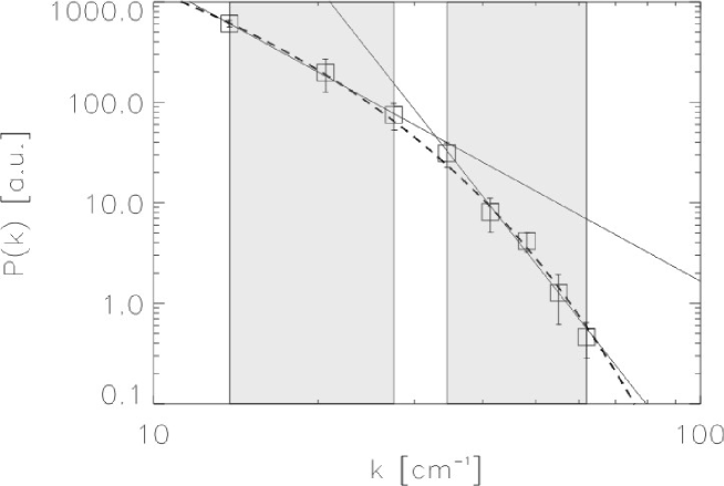
Figure 1: Wavenumber spectrum of broadband turbulence in W7-AS. Squares are measured points. Solid lines are power-law fits (Eq. (3)) and the dashed line is a fit to Eq. (1). The power-law fit grouping is indicated by the semi-transparent rectangles, the fit to Eq. (1) uses all data points.

A wavenumber spectrum of turbulence in W7-AS is shown in Fig. 1. The measured points are shown along with two power-law fits

$$P(k)\propto k^{-m},$$ (3)

where $m$ is a dimensionless constant. The power-law fits are shown as solid lines and an exponential fit to Eq. (1) is shown as a dashed line.

All fits shown in this paper have a normalized $\chi^{2}$ $\leq$ 1, ensuring the quality of the fits is good. The error bars are standard deviations and the semi-transparent rectangles indicate which points are included to make the fits.

The power-law fits are motivated by classical fluid turbulence theory where one expects wavenumber spectra to exhibit power-law behavior with exponents $m$ depending on the dimension of the observed turbulence:

• 3D: Energy is injected at a large scale and redistributed (cascaded) by nonlinear interactions down to a small dissipative scale. In this case, the energy spectrum in the inertial range $E(k)\propto k^{-5/3}$ [14].

• 2D: Here, two power-laws exist on either side of the energy injection scale. For smaller wavenumbers, the inverse energy cascade obeys $E(k)\propto k^{-5/3}$ and for larger wavenumbers, the enstrophy cascade follows $E(k)\propto k^{-3}$ [15].

• 1D: Energy is injected at a large scale and dissipated at a small scale; $E(k)\propto k^{-2}$ [16].

Our measured power is equivalent to the $d$-dimensional energy spectrum $F_{d}(k)$ [17, 14, 18]

$$P(k)=F_{d}(k)=\frac{E(k)}{A_{d}}$$

$$A_{1}=2\hskip 56.9055ptA_{2}=2\pi k\hskip 56.9055ptA_{3}=4\pi k^{2},$$ (4)

where $A_{d}$ is the surface area of a sphere having radius $k$ and dimension $d$. Usually on would assume that $d=2$ in fusion plasmas, since transport along magnetic field lines is nearly instantaneous. The fits to Eq. (3) in Fig. 1 yield exponents $m$ = 3.0 $\pm$ 0.4 (small wavenumbers) and 6.9 $\pm$ 0.7 (large wavenumbers). A similar behavior has previously been reported in Ref. [19] where it was speculated that the wavenumber value at the transition between the two power-laws should correspond to a characteristic spatial scale in the plasma. The only length scale close to the transitional value was found to be the ion Larmor radius $\rho_{i}$.

The spectrum at small wavenumbers is roughly consistent with the inverse energy cascade in 2D turbulence, $F_{2}(k)\propto k^{-8/3}$. The exponent at large wavenumbers does not fit into this framework. However, for very large wavenumbers one enters the dissipation range; here, it has been argued that the energy spectrum could have one of the following dependencies

$$E_{\rm Neumann}(k)\propto e^{-ak}\hskip 56.9055ptE_{\rm Heisenberg}(k)\propto k^{-7},$$ (5)

where $a>0$ is a constant having a dimension of length (see Ref. [16] and references therein). The energy spectrum proposed by J von Neumann was what initially inspired us to investigate an exponential decay of $P(k)$ in Ref. [12]. J von Neumann’s work on this topic is from 1949 and two years later, A A Townsend published a more generalized expression [20].

Fitting all wavenumbers to Eq. (1), $E_{\rm Neumann}(k)/A_{2}$, we find that $n$ = 0.11 $\pm$ 0.004 cm or a wavenumber of 57.1 cm^-1. Alternatively, the transitional wavenumber found at the intersection between the two power-laws is 32.8 cm^-1 (0.19 cm). The expression $E_{\rm Heisenberg}(k)/A_{2}$ yields $m$ = 8, which is close to the experimental value $m$ = 6.9 for large wavenumbers. Calculating the ion Larmor radius at the electron temperature $\rho_{s}$ for this case we find that it is 0.1 cm, i.e. the same order of magnitude as the spatial scales found above. We used $\rho_{s}$ instead of $\rho_{i}$ because ion temperature measurements were unavailable.

Currently we can think of three possible explanations for the behavior of the wavenumber spectrum:

1. We observe 2D turbulence and the transition between the two power-laws occurs at a spatial scale where the inverse energy cascade develops into the dissipation range. However, the enstrophy cascade is not accounted for in this case.

2. We observe 2D turbulence in the dissipation range described by Eq. (1) as proposed by J von Neumann.

3. Turbulence theory does not apply. The transition between two power-laws or the characteristic scale found using a single exponential function (Eq. (2)) indicates that one scale dominates the turbulent dynamics in the wavenumber range studied.

In measurements of 2D fluid turbulence, it has been demonstrated that the inverse energy and forward enstrophy cascades merge into a single power-law when the system transitions to being fully turbulent [21]. This might be the reason for the missing enstrophy cascade discussed in item (i) above.

2.2 Cosmology

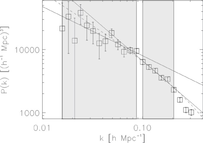
Figure 2: Wavenumber spectrum of galaxies measured by the SDSS Team. Squares are measured points. Solid lines are power-law fits (Eq. (3)), the dashed line is a fit to Eq. (1). The power-law fit grouping of points is chosen so the combined $\chi^{2}$ of the fits is minimized. The power-law fit grouping is indicated by the semi-transparent rectangles, the fit to Eq. (1) uses all data points up to $k$ = 0.2 h Mpc^-1. The data set is taken from Ref. [9].

The shape of the wavenumber spectrum shown in Fig. 1 bears a striking resemblance to measurements of fluctuations in the distribution of galaxies presented in Ref. [9], see Fig. 2. This motivates us to apply the analysis described in section 2.1 to the galaxy data. In section 2.2.1 we briefly put these measurements in context and then present an analysis of the galaxy wavenumber spectrum in section 2.2.2.

2.2.1 Inflation

Dramatic developments have taken place in cosmology over the last decade, lending increasing support to the paradigm of inflation as an explanation for what took place before the events described by the big bang theory [22]. Inflation solved the so-called horizon and flatness problems, but was at odds with earlier observations indicating that the ratio of the mass density of the universe to the critical value, the density parameter $\Omega$, was 0.2-0.3, while inflation predicted it should be 1:

$$\Omega=\frac{\rho}{\rho_{c}}$$

$$\Omega<1:{\rm open}\hskip 56.9055pt\Omega=1:{\rm flat}\hskip 56.9055pt\Omega>1:{\rm closed},$$ (6)

where $\rho_{c}=3H_{0}^{2}/8\pi G$ is the critical mass density, $H_{0}$ $\simeq$ 70 km/s/Mpc is the Hubble parameter observed today and $G$ is I Newton’s gravitational constant [23]. However, new measurements in the late 1990’s lead to a drastic modification of $\Omega$: Observations of type Ia supernovae (SN) showed that the separation velocity between galaxies was speeding up, not slowing down as would be expected for an open universe. The underlying explanation for this accelerated expansion is not understood, but it seems that the universe contains large quantities of negative pressure substance, creating a gravitational repulsion driving the expansion. This negative pressure material is called dark energy, the total density of dark energy $\Omega_{\Lambda}$ is 0.7. The existence of dark energy is equivalent to the cosmological constant $\Lambda$ introduced by A Einstein. The dark matter density $\Omega_{d}$ is 0.25 and the baryonic matter density $\Omega_{b}$ is 0.05, so the total density is very close (or equal) to the critical density. The SN Ia data is supported by measurements of nonuniformities in the cosmic microwave background (CMB) radiation. The CMB anisotropy is due to the presence of tiny primordial density fluctuations at the time of recombination, where atoms formed. At that point in time the age of the universe was about 400,000 years and the temperature was 3000 K. The structures observed in the CMB are called acoustic peaks, and the simplest versions of inflation all reproduce these structures quite accurately. The acoustic peaks can not be modelled by assuming that the universe is open.

2.2.2 SDSS wavenumber spectrum

A study of density fluctuations on large scales using 205,443 galaxies has been published by the SDSS Team in Ref. [9], see Fig. 2. 3D maps of the universe are provided by the SDSS galaxy redshift survey, observing about a quarter of the celestial sphere using a 2.5 m telescope and a charge-coupled device (CCD) camera. The galaxies had a mean redshift $z\approx$ 0.1, corresponding to light emitted 1-2 Gyr ago [23]. Fixing some cosmological parameters to Wilkinson Microwave Anisotropy Probe (WMAP) satellite values [24] one finds - using physics based models - that the wavenumber spectrum measurements were fitted by a matter density $\Omega_{m}=\Omega_{d}+\Omega_{b}=0.295\pm 0.0323$. In this case $h=H_{0}$/(100 km/s/Mpc) = 0.72 was assumed and it was observed that the wavenumber spectrum was not well characterized by a single power-law.

A follow-up paper by the SDSS Team, Ref. [25], combined non-CMB measurements (SDSS) with CMB measurements (WMAP) to constrain free parameters of cosmological models and break CMB degeneracies in parameter space. This resulted in $\Omega_{m}=0.30\pm 0.04$ and $h=0.70_{-0.03}^{+0.04}$. Adding the SDSS information more than halved WMAP-only error bars on some parameters, e.g. the Hubble parameter and matter density.

The data presented in Fig. 2 has been taken from M Tegmark’s homepage [26]. According to the recommendation by the SDSS Team [9], the three largest wavenumbers shown are not used in the fits described in this section.

As we did for the W7-AS data in Section 2.1, we fit the SDSS measurements to two power-laws (Eq. (3)) or the exponential function with an algebraic pre-factor (Eq. (1)). The power-law fits are shown as solid lines, the exponential fit as a dashed line.

The power-law fits yield exponents $m$ = 0.8 $\pm$ 0.03 (small wavenumbers) and 1.4 $\pm$ 0.1 (large wavenumbers). The wavenumber ranges were determined by minimizing the combined $\chi^{2}$ of the fits. As the SDSS Team found, a single power-law can not describe the observations. The exponents are not close to the ones governing fluid turbulence discussed in section 2.1. The transitional wavenumber (power-law intersection) is 0.07 h Mpc^-1, corresponding to a length of 89.8 h^-1 Mpc.

We find the characteristic length from Eq. (1) to be $n$ = 2.3 $\pm$ 0.5 h^-1 Mpc or a wavenumber of 2.7 h Mpc^-1.

3 Analysis of additional measurements

In Ref. [11] we noted that both fusion plasma and cosmological wavenumber spectra peak at small wavenumbers and decrease both above and below that peak. In this section we analyze supplemental measurements on a wider range of scales. The fusion plasma measurements were made in a tokamak, so our explicit assumption is that turbulence in stellarators and tokamaks is comparable.

We fit the data to a modified version of Eq. (1), namely

$$P(k)\propto\frac{1}{k^{\alpha}}\times e^{-nk},$$ (7)

where $\alpha$ is brought in as an additional fit parameter. The introduction of $\alpha$ is based on the assumed functional form of the energy spectrum in the dissipation range of fluid turbulence [27]. Further, since we have no clear criteria for choosing between Eqs. (1) and (2), leaving $\alpha$ to be fitted will test our biased opinion in Ref. [11] for Eq. (1). Using Eq. (4), Eq. (7) implies that $E(k)$ $\propto$ $k^{(d-1)-\alpha}\times e^{-nk}$.

3.1 Tokamak fusion plasma

We analyze density fluctuations at small wavenumbers in C-Mod using the PCI diagnostic. Measurements in the low confinement mode taken from Fig. 11 in Ref. [28] are shown in Fig. 3. The dashed line shows the fit made using Eq. (7) which yields $n$ = 0.11 $\pm$ 0.005 cm and $\alpha$ = 0.30 $\pm$ 0.02. The size of $n$ is close to the value of $\rho_{s}$ in the given plasma.

3.2 Cosmological wavenumber spectrum

The expanded cosmological data set shown in Fig. 38 of Ref. [9] is re-plotted in Fig. 4. These measurements have been provided by M Tegmark [10]. They are a combination of the measured density fluctuation power using several diagnostic techniques; the dashed line is a fit to a current model in cosmology, the so-called ”vanilla light” flat adiabatic $\Lambda$CDM model with negligible tilt, running tilt, tensor modes or massive neutrinos [9, 25].

During our analysis of the measurements it became obvious that Eq. (7) does not fit the entire range of wavenumbers above the peak of the spectrum. Therefore two fits were made:

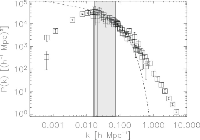
Figure 5: Wavenumber spectrum of the combined cosmological measurements. Squares are measured points. The dashed line is a fit to Eq. (7) using the data indicated by the semi-transparent rectangle. The measurements are taken from Ref. [9].

• A small wavenumber fit where the smallest wavenumber used is chosen to be the one closest to (but larger than) the peak of the $\Lambda$CDM model shown in Fig. 4. The largest wavenumber used is chosen so that $\chi^{2}$ of the fit is 1. In Fig. 5 the fit is displayed as a dashed line. The parameters found are $n$ = 13.3 $\pm$ 1.6 h^-1 Mpc and $\alpha$ = 0.24 $\pm$ 0.06. Note the interesting proximity of this $\alpha$ to the result in section 3.1.

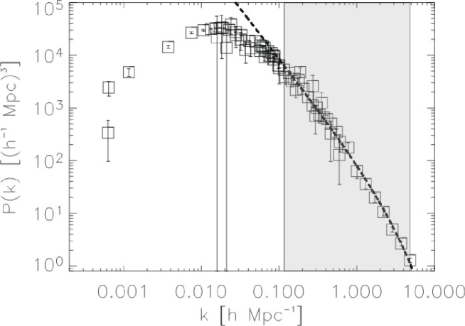
Figure 6: Wavenumber spectrum of the combined cosmological measurements. Squares are measured points. The dashed line is a fit to Eq. (7) using the data indicated by the semi-transparent rectangle. The measurements are taken from Ref. [9].

• A large wavenumber fit where the largest wavenumber used is the maximum of the data set and the smallest wavenumber is chosen so that $\chi^{2}$ of the fit is 1. In Fig. 6 the fit is displayed as a dashed line. The parameters found are $n$ = 0.33 $\pm$ 0.05 h^-1 Mpc and $\alpha$ = 1.90 $\pm$ 0.05.

The wavenumbers not being used in either fit define a transitional region: [0.08, 0.10] h Mpc^-1. This interval is in rough agreement with the transition found between the two power-law fits shown in Fig. 2.

4 Revised analysis of stellarator fusion plasmas

Based on the insights gained in section 3, we revisit the turbulence measurements made in W7-AS, see Fig. 1. Our approach is to make three fits, one for small, one for large and one for all wavenumbers:

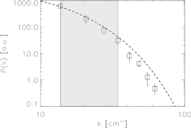
Figure 7: Wavenumber spectrum of broadband turbulence in W7-AS. Squares are measured points. The dashed line is a fit to Eq. (7) using the measurements indicated by the semi-transparent rectangle. Note that this is exclusively an amplitude fit, we use $n$ and $\alpha$ from the PCI fit, see section 3.1 and Fig. 3.

• For the fit to small wavenumbers we use $n$ and $\alpha$ found from the PCI measurements in section 3.1 and only allow the overall amplitude to vary. The largest wavenumber to be included in the fit is chosen so that $\chi^{2}$ of the fit is 1. Using this criterion the four smallest wavenumbers are utilized. In Fig. 7 the fit is shown as a dashed line.

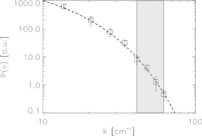
Figure 8: Wavenumber spectrum of broadband turbulence in W7-AS. Squares are measured points. The dashed line is a fit to Eq. (7) using the measurements indicated by the semi-transparent rectangle.

• We allow all fit parameters in Eq. (7) to vary for the fit to the four largest wavenumbers and show the resulting fit as a dashed line in Fig. 8. The fit yields $n$ = 0.14 $\pm$ 0.008 cm and $\alpha$ = 0.25 $\pm$ 0.1. This fit is also good for the entire wavenumber range: Using the found parameters, $\chi^{2}$ remains less than 1 for all eight wavenumbers.

• Fit to Eq. (7) using all eight wavenumbers and allowing every fit parameter to vary. The fit yields $n$ = 0.14 $\pm$ 0.007 cm and $\alpha$ = 0.11 $\pm$ 0.2, which is consistent with a pure exponential function (Eq. (2)).

The amplitude-only fit using PCI parameters indicates a transition at the center of the data set, whereas the two other fits suggest that the data is consistent with a continuous behavior. It is apparent that additional measurements at large wavenumbers in fusion plasmas are needed to gain confidence in the fits. Some of the existing points might be in a transitional region akin to the one found in the cosmological data.

5 Discussion

The fact that density fluctuations on small (fusion plasmas) and large (cosmological) scales can be described by an exponential function with an algebraic pre-factor, Eq. (7), might indicate that plasma turbulence at early times has been expanded to cosmological proportions. A natural consequence of that thought would be to investigate fluctuations in quark-gluon plasmas (QGPs) corresponding to even earlier times. However, experimental techniques to do this are not sufficiently developed at the moment due to the extreme nature of QGPs. It has been suggested that complex (or dusty) plasmas could be used as a model of QGPs [29].

It is fascinating that wavenumber spectra over wider scales peak at small wavenumbers and decrease both above and below that peak. This is seen both in fusion plasmas and on cosmological scales, compare Figs. 3 and 4. Turbulence theory in 1D or 3D would interpret the peak position as the scale where energy is injected.

Fitting wavenumber spectra to power-laws as we did in section 2 is based on fluid turbulence theories, but in general care must be taken when interpreting the outcome: We know that an exponential function can be Taylor expanded to a Maclaurin series

$$P(k)\propto e^{-nk}=\sum_{i=0}^{\infty}\frac{(-nk)^{i}}{i!}.$$ (8)

So locally, i.e. for a small range of wavenumbers, an exponential dependency can be masked as a power-law; the exponent would vary as a function of the wavenumber range selected. To some extent this objection also holds true for our results using Eq. (7) to identify two wavenumber intervals having different fit parameters. It is an open question whether an extension of the cosmological data to larger wavenumbers would necessitate further intervals. However, in fluid turbulence simulations a transition between near- and far-dissipation similar to the one we discuss has been identified [30]. This observation lends support to the interpretation that our dual fits describe different types of dissipation.

To sum up, we favor Eq. (7) as a descriptor of the data, both for fusion plasma and cosmological measurements. Perhaps forcing occurs at a large scale where the spectra peak and transitions directly to dissipation. The fact that we obtain $n\simeq\rho_{s}$ using Eq. (7) for fusion plasmas suggests that $n$ is the characteristic scale of turbulence.

We would like to point out that observations of electric field fluctuations in the solar wind are found to be proportional to exp($-k\rho_{i}$/12.5) for $k\rho_{i}$ $>$ 2.5 [31]. It should be noted that the electric field measurements at these large wavenumbers are noisy. Work on the solar wind data to analyze density fluctuations is in progress [32].

6 Conclusions

We have in this paper reported on suggestive similarities between density fluctuation power versus wavenumber on small (mm) and large (Mpc) scales.

The small scale measurements were made in fusion plasmas and compared to predictions from turbulence theory. The data sets fit Eq. (7), which has a functional form that can be explained as dissipation by turbulence theory. The large scale cosmological measurements can also be described by Eq. (7). In general, two wavenumber ranges separated by a transitional region are identified.

The similar dependency of density fluctuation power on wavenumber might indicate a common origin of these fluctuations, perhaps from fluctuations in QGPs at early stages in the formation of the universe. The value of $\alpha$ is almost identical for both fusion plasma and cosmological measurements at wavenumbers close to but above the peak of the spectra.

To progress further, it is essential that the quantity of wavenumber-resolved fusion plasma turbulence measurements is vastly increased.

References

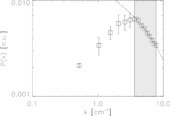
Figure 3: Wavenumber spectrum of broadband turbulence in C-Mod. Squares are measured points. The dashed line is a fit to Eq. (7) using the measurements indicated by the semi-transparent rectangle.

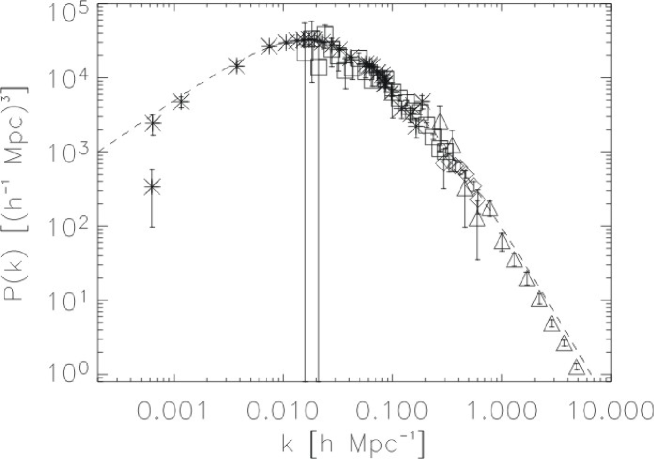
Figure 4: Wavenumber spectrum of the combined cosmological measurements. Asterisks are CMB radiation, squares are SDSS, plus is cluster abundance, diamonds are weak lensing and triangles are Lyman-$\alpha$ forest measurements. The dashed line is a fit to the $\Lambda$CDM model. The data sets are taken from Ref. [9].

References

- [1] Wootton A J et al 1990 Phys. Fluids B 2 2879
- [2] Hinton F L and Hazeltine R D 1976 Rev. Mod. Phys. 48 239
- [3] Saffman M et al 2001 Rev. Sci. Instrum. 72 2579
- [4] Basse N P 2002 Ph.D. Thesis, University of Copenhagen http://www.risoe.dk/rispubl/ofd/ris-r-1355.htm
- [5] Renner H et al 1989 Plasma Phys. Control. Fusion 31 1579
- [6] Mazurenko A et al 2002 Phys. Rev. Lett. 89 225004
- [7] Hutchinson I H et al 1994 Phys. Plasmas 1 1511
- [8] http://www.sdss.org/
- [9] Tegmark M et al 2004 Astrophys. J. 606 702
- [10] Tegmark M 2005 Private communication
- [11] Basse N P 2005 Phys. Lett. A 340 456
- [12] Basse N P et al 2002 Phys. Plasmas 9 3035
- [13] Hennequin P et al 2004 Plasma Phys. Control. Fusion 46 B121
- [14] Frisch U 1995 Turbulence (Cambridge: Cambridge University Press)
- [15] Antar G et al 1998 Plasma Phys. Control. Fusion 40 947
- [16] von Neumann J 1963 Collected works VI: Theory of games, astrophysics, hydrodynamics and meteorology, ed Taub A H (Oxford: Pergamon Press)
- [17] Tennekes H and Lumley J L 1972 A first course in turbulence (Cambridge: MIT Press)
- [18] Antar G 1996 Ph.D. Thesis, École Polytechnique
- [19] Honoré C et al 1998 Proc. 25th EPS Conf. on Controlled Fusion and Plasma Physics (Prague, Czech Republic) 22C 647
- [20] Townsend A A 1951 Proc. Royal Soc. London, Ser. A 208 534
- [21] Shats M G et al 2005 Phys. Rev. E 71 046409
- [22] Guth A H and Kaiser D I 2005 Science 307 884
- [23] Kinney W H 2004 arXiv:astro-ph/0301448
- [24] Spergel D N et al 2003 Astrophys. J., Suppl. Ser. 148 175
- [25] Tegmark M et al 2004 Phys. Rev. D 69 103501
- [26] M Tegmark’s homepage is http://space.mit.edu/home/tegmark/ and the SDSS data used is available from http://space.mit.edu/home/tegmark/sdsspower/sdss_measurements.txt
- [27] Chen S et al 1993 Phys. Rev. Lett. 70 3051
- [28] Basse N P et al 2005 Phys. Plasmas 12 052512
- [29] Thoma M H 2005 arXiv:hep-ph/0509154
- [30] Martínez D O et al 1997 J. Plasma Phys. 57 195
- [31] Bale S D et al 2005 Phys. Rev. Lett. 94 215002
- [32] Bale S D 2005 Private communication