Hydrodynamic flow patterns and synchronization of beating cilia

Abstract

We calculate the hydrodynamic flow field generated far from a cilium which is attached to a surface and beats periodically. In the case of two beating cilia, hydrodynamic interactions can lead to synchronization of the cilia, which are nonlinear oscillators. We present a state diagram where synchronized states occur as a function of distance of cilia and the relative orientation of their beat. Synchronized states occur with different relative phases. In addition, asynchronous solutions exist. Our work could be relevant for the synchronized motion of cilia generating hydrodynamic flows on the surface of cells.

Many eucaryotic cells possess cilia, which are motile, whip-like structures on the cell surface Bray (2001); Brennen and Winet (1977). While certain cells such as sperm swim using a single cilium (in this case called flagellum) other cells use several or a large number of cilia for propulsion in a fluid. Epithelial cells such as those in the respiratory tract use densely ciliated surfaces to transport fluids. Hydrodynamic flows generated by cilia also play a key role during the morphogenesis of higher organisms. In mammals, the left-right symmetry of the embryo is broken with the help of nodal cilia which generate a hydrodynamic flow to one side which transports signaling molecules and breaks the symmetry McGrath and Brueckner (2003); Cartwright et al. (2004); Okada et al. (2005). All these cilia are based on the same structure, called the axoneme, which is built of a very regular arrangement of protein filaments called microtubules in a cylindrical geometry. Motility is achieved by the action of a large number of dynein motor proteins which generate forces in the cilium while consuming a chemical fuel. As a consequence, the cilium produces periodic deformations in three dimensional space.

Cilia in different organisms differ mainly by their length and their pattern of beating. They typically measure few micrometers up to a few tens of micrometers in length and around $150-300\,\rm nm$ in diameter. While the beat of sperm tails is typically a planar, sometimes helical wave, more complex, three dimensional, asymmetric beating patterns occur typically in cells which propel fluids along surfaces. In this case, the working cycle of a cilium consists of a fast, upright, effective stroke and a recovery stroke which brings the cilium more slowly back to the original position on a path closer to the surface, see Fig. 1a. Nodal cilia break the left-right symmetry of developing embryos by generating rotatory motion in a plane tilted with respect to the surface to which they are attached Okada et al. (2005).

In this letter, we discuss the hydrodynamic flow field generated by a single cilium which beats in an asymmetric pattern while attached to a surface. While the near field of the hydrodynamic flow depends on the detailed beating pattern and the whip-like geometry of the cilium, the far field has general features which only depend on a few parameters characterizing the symmetry of the beat. Using the flow field generated by a beating cilium, we study the hydrodynamic interaction between two cilia. We discuss conditions that lead to synchronization of the two cilia by hydrodynamic interactions.

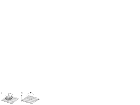
Figure 1: a) Beating pattern of a cilium. The effective stroke and the recovery stroke are different (arrows) and a net flow is generated. b) Simplified representation of the cilium by a small sphere, moving on a tilted elliptical trajectory.

Our minimal model of the ciliary beat (Fig. 1b) captures the essential features and symmetries - the difference between effective stroke and recovery stroke of whip-like beating as well as the tilted rotatory motion of nodal cilia. We replace the cilium by a small sphere of radius $a$ (essentially describing the center of mass position of the cilium), which moves on a fixed trajectory in the vicinity of a planar surface (defined as the plane $z=0$). The trajectory of the bead is elliptic, the phase of the oscillation (the position along the trajectory) is described by an angle $\phi$. The asymmetry of the ciliary beat is reflected in the fact that the two principal axes (denoted $A$ and $B$) are different, and that the ellipse is tilted with respect to the surface as described by the parameter $C$. The position of the sphere is given by

$$\mathbf{x}_{i}=\mathbf{x}_{i}^{0}+\mathbf{x}(\phi_{i})={\left(\begin{array}[]{c}x_{i}^{0}\\ y_{i}^{0}\\ 0\end{array}\right)}+\left(\begin{array}[]{c}A\cos\phi_{i}\\ B\sin\phi_{i}\\ D+C\cos\phi_{i}\end{array}\right)$$ (1)

here, $x_{i}^{0}$ and $y_{i}^{0}$ describes the position on the surface at which the cilium is attached. For more detailed descriptions of the ciliary beat see, e.g., refs. Brennen and Winet (1977); Gueron and Levit-Gurevich (1998).

The viscous, over damped fluid around the cilium can be described by the Stokes equation for the hydrodynamic flow field ${\bf v}$

$$\eta\nabla^{2}{\bf v}=\nabla P$$ (2)

where the pressure $P$ is a Lagrange multiplier to impose the constraint of incompressibility, $\nabla\cdot{\bf v}=0$. The far-field generated by a moving sphere in the vicinity of a surface can be calculated by studying the solution of the Stokes equation to a delta-distributed force ${\bf F}_{i}$ at position ${\bf x}_{i}=(x_{i},y_{i},z_{i})$ which is of the form $\mathbf{v}(\mathbf{x})=\tensor{G}(\mathbf{x}_{i},\mathbf{x})\mathbf{F}_{i}$. The tensor $\tensor{G}$ consists of a stokeslet $\tensor{G}^{S}$, which describes the velocity field around a small isolated particle, and an image, required to satisfy the no-slip boundary condition on the surface Blake (1971). The image is located at the particle position, mirrored over the boundary plane, $\mathbf{\bar{x}}_{i}=\mathbf{x}_{i}-2z_{i}\hat{e}_{z}$, and consists of an anti-stokeslet, a source-doublet $G^{D}$ and a stokes-doublet $G^{SD}$, so that $\tensor{G}(\mathbf{x}_{i},\mathbf{x})=\tensor{G}^{S}(\mathbf{x}-\mathbf{x}_{i})-\tensor{G}^{S}(\mathbf{x}-\mathbf{\bar{x}}_{i})+2z_{i}^{2}\tensor{G}^{D}(\mathbf{x}-\mathbf{\bar{x}}_{i})-2z_{i}\tensor{G}^{SD}(\mathbf{x}-\mathbf{\bar{x}}_{i})$ with

$$G_{\alpha\beta}^{S}(\mathbf{x}) =\frac{1}{8\pi\eta}\left(\frac{\delta_{\alpha\beta}}{\left|\mathbf{x}\right|}+\frac{\mathbf{x}_{\alpha}\mathbf{x}_{\beta}}{\left|\mathbf{x}\right|^{3}}\right)$$ (3)

$$G_{\alpha\beta}^{D}(\mathbf{x}) =\frac{1}{8\pi\eta}(1-2\delta_{\beta z})\frac{\partial}{\partial x_{\beta}}\left(\frac{x_{\alpha}}{\left|\mathbf{x}\right|^{3}}\right)$$ (4)

$$G_{\alpha\beta}^{SD}(\mathbf{x}) =(1-2\delta_{\beta z})\frac{\partial}{\partial x_{\beta}}G_{\alpha z}^{S}(\mathbf{x})\;.$$ (5)

The leading behavior of $G$ which describes the far-field (for $r\gg z_{i},z$) can be written as

$$\tensor{G}(\mathbf{x}_{i},\mathbf{x})\approx\frac{3}{2\pi\eta}\frac{z_{i}z}{r^{3}}\left(\begin{matrix}\cos^{2}\beta&\sin\beta\cos\beta&0\\ \sin\beta\cos\beta&\sin^{2}\beta&0\\ 0&0&0\end{matrix}\right)$$ (6)

where $\tan\beta=(y_{i}-y)/(x_{i}-x)$ and $r^{2}=(x_{i}-x)^{2}+(y_{i}-y)^{2}$. For constant height $z$, $G$ decays as as $G\propto r^{-3}$.

We assume that the active mechanism in the cilium generates a tangential force ${\bf f}_{i}=f_{i}\hat{\mathbf{t}}_{i}$. In a simplified model, it is a linear function of the velocity ${\bf v}_{i}=v_{i}\hat{\mathbf{t}}_{i}$ described by $f_{i}=f_{0}-\kappa v_{i}$. Here, $\hat{\mathbf{t}}_{i}$ is a normalized vector parallel to ${\bf t}_{i}=d{\bf x}_{i}/d\phi_{i}$. Note that the total force ${\bf F}_{i}$ acting on the sphere is in general not parallel to the direction of motion since normal forces arise to establish the constraint which keeps the sphere moving on the ellipsoidal track. The force ${\bf F}_{i}$ thus obeys

$$\hat{\mathbf{t}}_{i}\cdot{\bf F}_{i}=f_{0}-\kappa v_{i}\;.$$ (7)

This force is balanced by hydrodynamic friction $\mathbf{F}_{i}=\tensor{\gamma}_{i}\mathbf{v}_{i}$, where the friction matrix is given by Dufresne et al. (2000)

$$\tensor{\gamma}_{i}=\tensor{\gamma}(\mathbf{x}_{i})=\gamma_{0}\left(\tensor{I}+\frac{9}{16}\frac{a}{z_{i}}\left(\begin{array}[]{ccc}1&&\\ &1&\\ &&2\end{array}\right)\right)\;.$$ (8)

Here $\gamma_{0}=6\pi\eta a$ denotes the Stokes friction of a small sphere with radius $a$ and the second term the corrections due to proximity of the plane. The force-velocity relation (7), balanced by the friction force leads to the equation of motion for the phase of oscillation

$$\frac{d\phi_{i}}{dt}=f_{0}\left(\hat{\mathbf{t}}_{i}\cdot\tensor{\gamma}(\mathbf{x}_{i})\mathbf{t}_{i}+\kappa\hat{\mathbf{t}}_{i}\cdot\mathbf{t}_{i}\right)^{-1}$$ (9)

The resulting motion of the sphere is periodic in time. In the limit of small radius $a$, the friction coefficient becomes independent of the height over the surface and the period is $T=\frac{2\pi}{\omega}\simeq\frac{(\kappa+\gamma_{0})\ell}{f_{0}}$, where $\ell$ denotes the trajectory length. The phase $\phi_{0}$ of the sphere as a function of time can be written as

$$\phi_{0}(\omega t)=\omega t+K\sin(\omega t)+L\sin(2\omega t)+\ldots$$ (10)

The coefficient $L$ is related to the eccentricity of the ellipse (if the particle moves at a constant speed, the parameter $\phi$ has a variable time derivative) and thus depends on the geometry of the trajectory. The coefficient $K\propto aC/D^{2}$, describes variations of the velocity due to variations of the friction (8) resulting form varying distance of the particle from the surface.

We can now obtain the hydrodynamic far-field of a beating cilium ${\bf v}({\bf x},t)=\tensor{G}({\bf x}_{i}(t),{\bf x})\tensor{\gamma}_{i}(\mathbf{x}_{i}(t)){\mathbf{v}}_{i}(t)$. Averaging over one period, we define the net flow $\bar{\bf v}({\bf x})=\frac{1}{T}\int_{0}^{T}\mathbf{v}(\mathbf{x},t)dt=\frac{1}{T}\oint\tensor{G}({\bf x}_{i},{\bf x})\tensor{\gamma}_{i}(\mathbf{x}_{i})d\mathbf{x}_{i}$. It only depends on the period and the shape of the trajectory, but not on details in the phase $\phi_{0}(t)$. Because the sphere causes a stronger fluid motion when it is further away from the surface (during the working stroke) than when it is closer (recovery stroke), it causes a net fluid flow in $y$ direction. Examples of flux lines of the time-averaged fluid flow generated in this way are displayed in Fig. 2. Far from a sphere moving around the center at $x_{i}^{0}=0$, $y_{i}^{0}=0$, the average velocity field is given by

$$\bar{\mathbf{v}}=\frac{9\pi aBC}{T}\frac{yz}{\left|\mathbf{x}\right|^{5}}\left(\begin{array}[]{c}x\\ y\\ z\end{array}\right)$$ (11)

Note that it only depends on the sphere radius $a$, the period $T$ and the projected area of the trajectory to the $y$-$z$ plane, $\pi BC$. Corrections to this flow field can be neglected in the far field since they decay at least as ${\cal O}(|\mathbf{x}|^{3})$ Lenz et al. (2003).

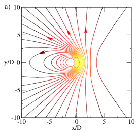
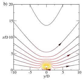
Figure 2: a) Flux lines describing the time averaged fluid flow generated by a sphere moving on a tilted elliptical path shown in the $x-y$ plane for $z/D=2$ (other parameters: $A/D=0.5$, $B/D=1$, $C/D=0.5$, $a/D=0.1$). The curves were obtained numerically using the flow field based on Eqns. (3)-(5). b) Same flow field displayed in the $y$-$z$ plane, for $x=0$. Black lines correspond to low fluid velocity, yellow lines to high velocity. The dashed lines indicate the projections of the sphere trajectory.

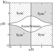
Figure 3: a) Top view of the arrangement of two elliptical trajectories which represent two beating cilia. The distance $r$ and the angle $\beta$ are indicated. b) The state diagram as a function of the distance vector $x=x_{2}^{0}-x_{1}^{0}$, $y=y_{2}^{0}-y_{1}^{0}$, determined from the numerical solution of the full model equations. Three different regions are indicated. In the region of asynchronous beat, two frequencies occur. Two synchronous states can be distinguished with equal (Sync⁺) and opposite (Sync^-) phase of both cilia in the limit of large separation $r$.

We now turn to the case of two beating cilia which interact hydrodynamically. The force ${\bf F}_{2}$ the second sphere exerts on the fluid at position ${\bf x}_{2}$ generates hydrodynamic flows at position ${\bf x_{1}}$ and thus influences the force ${\bf F}_{1}$ exerted by the first sphere:

$${\mathbf{F}}_{1}=\tensor{\gamma}_{1}\left(\mathbf{v}_{1}-\tensor{G}(\mathbf{x}_{2},\mathbf{x}_{1})\mathbf{F}_{2}\right)$$ (12)

This equation can be used to define the dynamics of motion of both spheres along their ellipsoidal trajectories in the following manner. We assume again that each sphere is driven by a force obeying Eq. (7). Eq. (12) together with the corresponding equation for ${\bf F}_{2}$ then uniquely determines the tangential velocities of both spheres $v_{i}=\hat{\mathbf{t}}_{i}\cdot{\bf v}_{i}$. This allows us to set up the equations of motion that determine the time derivatives $\dot{\phi}_{1}$ and $\dot{\phi}_{2}$ as functions of $\phi_{1}$ and $\phi_{2}$. The problem of two coupled phase oscillators is equivalent to the Kuramoto model Kuramoto (1984), a classical model for describing synchronization phenomena Pikovsky et al. (2001). Performing numerical solutions to these dynamic equations, we find that for certain parameter values, after long times the motion of both spheres becomes periodic with the same frequency and the oscillations thus synchronize. A synchronized state is characterized by the phase lag $\delta=\left<\phi_{2}-\phi_{1}\right>$, where the brackets denote a time average over one period. Regions of synchronous states and a region of asynchronous states are indicated in the state diagram of Fig. 3b. The two regions of synchronous states correspond to equal and opposite phases in the limit of infinite separation $r$. The values of $\delta$ are displayed in Fig. 4 as a function of the angle $\beta$ for different distances $r=|{\bf x}_{1}^{0}-{\bf x}_{2}^{0}|$ between the two cilia. For some intervals of $\beta$, no synchronized solution occurs and the spheres rotate in an asynchronous manner with two different frequencies. Note that even if both cilia have identical properties, the arrangement shown in Fig 3a breaks the symmetry and both cilia can have different preferred frequencies when they interact.

The existence and stability of synchronous states can be studied analytically. First, using Eq. (12), we find for large $r\gg a$

$$f_{0} = \hat{\mathbf{t}}_{1}\cdot(\tensor{\gamma}(\mathbf{x}_{1})+\kappa\tensor{I})\mathbf{v}_{1}-\hat{\mathbf{t}}_{1}\cdot\tensor{\gamma}(\mathbf{x}_{1})\tensor{G}(\mathbf{x}_{2},\mathbf{x}_{1})\tensor{\gamma}(\mathbf{x}_{2})\mathbf{v}_{2}$$ (13)

$$+\mathcal{O}\left(\frac{f_{0}a^{2}D^{4}}{r^{6}}\right)$$

Here, we have used the fact that for large $r\gg a$, the interactions decay as $G\propto r^{-3}$, while the friction terms scale with the sphere size, $\gamma\propto a$. Using this relation between the tangential velocities, we can study synchronization. For an isolated sphere, the phase as a function of time is denoted $\phi_{0}(t)$ (10). We denote by $\phi_{1}(t)$ the phase of a sphere 1 when interacting with sphere 2. The variation $\Delta T$ of the oscillation period $T$ of sphere 1 can then be written as

$$\Delta T = \int_{0}^{2\pi}\left(\frac{1}{\dot{\phi}_{1}(\phi)}-\frac{1}{\dot{\phi}_{0}(\phi)}\right)d\phi=\int_{0}^{T_{0}}\frac{v_{0}-v_{1}}{v_{0}}dt$$ (14)

$$\approx -\frac{1}{f_{0}}\int_{0}^{T_{0}}\hat{\mathbf{t}}_{1}\cdot\tensor{\gamma}(\mathbf{x}_{1})\tensor{G}(\mathbf{x}_{2},\mathbf{x}_{1})\tensor{\gamma}(\mathbf{x}_{2})\hat{\mathbf{t}}_{2}\,v_{2}\,dt$$

where the last expression becomes correct in the limit of large $r/a$. In this limit, the variation $\Delta T$ can be calculated using the Ansatz $\mathbf{x}_{1}=\mathbf{x}_{1}^{0}+\mathbf{x}(\phi_{0}(\omega t))$ and $\mathbf{x}_{2}=\mathbf{x}_{2}^{0}+\mathbf{x}(\phi_{0}(\omega t+\delta))$ resulting in a function $\Delta T(r,\beta,\delta)$. A synchronized steady state exists if the change in period due to interactions is the same for both spheres, i.e., $\Delta T(r,\beta,\delta)=\Delta T(r,\beta+\pi,-\delta)$, where we have taken into account that exchanging both spheres corresponds to $\beta\rightarrow\beta+\pi$ and $\delta\to-\delta$, see Fig. 3a. Furthermore, a synchronized steady state is locally stable if $\partial/\partial\delta[\Delta T(r,\beta,\delta)-\Delta T(r,\beta+\pi,-\delta)]<0$. In order to find explicit expressions for $\Delta T$, we perform a systematic expansion in the small parameter $K$. In the limit of vanishing radius $a$, the friction matrix $\tensor{\gamma}$ becomes independent of the height $z$. The velocity of a single sphere then becomes constant along the trajectory ($K=0$). As a consequence, the corresponding variation $\Delta T_{0}$ of the period, resulting from Eq. (14), becomes symmetric with respect to $\delta\to-\delta$ as well as with respect to $\beta\to\beta+\pi$ and the condition that both particles have the same period is satisfied trivially, regardless of the phase lag $\delta$. In order to find nontrivial synchronized states, we have to go to first order in $K$

Figure 4: The phase difference $\delta$ between two spheres on elliptic trajectories in the stable stationary state as a function of their relative position in polar coordinates (angle $\beta$, distance $r$) obtained by numerical solutions to the full dynamic equations. In the limit $r\to\infty$ analytic far-field calculations show that only equal and opposite phases ($\delta=0$ and $\pm\pi$, respectively) occur. For smaller $r$, nontrivial angles $\delta$ occur. Synchronous states become unstable where the lines end (black dots). Between these points motion is asynchronous.

where

$$\Delta T=\Delta T_{s}-T_{0}\frac{9\pi^{2}\gamma_{0}aABCDK}{{2(\gamma_{0}+\kappa)}\ell^{2}r^{3}}\sin 2\beta\sin\delta$$ (15)

($\Delta T_{s}(\delta)\equiv\Delta T_{s}(-\delta)$ represents symmetric terms that are irrelevant for synchronization). At this order in $a$ and $r$, the condition for a stable synchronized steady state is fulfilled with $\delta=0$ for $0<\beta<\pi/2$ and $\pi<\beta<3\pi/2$ and with $\delta=\pi$ for $\pi/2<\beta<\pi$ and $3\pi/2<\beta<2\pi$. This is consistent with our numerical solutions in the limit of large $r$, see Fig. 4. For smaller distance $r$, the contribution of terms proportional $r^{-4}$ becomes relevant.

To conclude, we have shown that the hydrodynamic far field around a periodically beating cilium has generic properties which do not depend on the detailed beating pattern. Its main features can thus be generated by a sphere moving on a tilted elliptical trajectory. This captures the asymmetry of the ciliary beat. As a consequence, the resulting flow is a time periodic pattern superimposed on a time-independent net flow. If the beating cilium is perturbed by external forces, this interferes with the internal force generating process and affects the instantaneous angular velocity of oscillations. We capture this effect by a linear relationship between external force and the velocity $v$ of the sphere. The force exerted on one cilium by the hydrodynamic flow generated by the other couples both oscillators. The resulting synchronization phenomena depend on the distance $r$ between cilia but also the parameters $a/D$ and $a/C$ which characterize the difference of effective and recovery strokes. No synchronization occurs if the motion is rotationally symmetric or helical Kim and Powers (2004); Reichert and Stark (2005).

A natural extension of our study is the generalization to a periodic lattice of cilia attached to a surface. Such situations correspond to some epithelial cells which generate fluid flows on their surface and to microorganisms such as paramecium. In all these cases, the ciliary beat is organized in metachronal waves which result from hydrodynamic and steric interactions between cilia. In different cells, these waves of ciliary strokes propagate along the surface in different directions relative to the one defined by the working stroke Machemer (1972); Gheber and Priel (1997). Other examples for hydrodynamically stirred surfaces are realized in experiments where bacteria are attached to a surface by their flagella which are driven by rotatory motors Darnton et al. (2004). Each bacterium in this system could be represented by a rotating sphere as in our description. In principle, the synchronization effects between two rotating elements discussed here could be studied in such experiments. The extension of our study to many hydrodynamically coupled cilia and the description of metachronal waves and other collective modes is left for future work.