A ring trap for ultracold atoms

Abstract

We propose a new kind of toroidal trap, designed for ultracold atoms. It relies on a combination of a magnetic trap for rf-dressed atoms, which creates a bubble-like trap, and a standing wave of light. This new trap is well suited for investigating questions of low dimensionality in a ring potential. We study the trap characteristics for a set of experimentally accessible parameters. A loading procedure from a conventional magnetic trap is also proposed. The flexible nature of this new ring trap, including an adjustable radius and adjustable transverse oscillation frequencies, will allow the study of superfluidity in variable geometries and dimensionalities.

I Introduction

In recent years, much work has been devoted to study theoretically and experimentally ultra cold neutral atoms in very elongated traps, where the atomic cloud approaches the one-dimensional regime Petrov ; Goerlitz01 ; Dettmer01 ; Richard03 ; Shvarchuck02 ; Moritz03 ; Laburthe04 ; Paredes04 . The situation under consideration is usually a one dimensional harmonic oscillator, either a single trap Goerlitz01 ; Dettmer01 ; Richard03 ; Shvarchuck02 or a series of such harmonic traps Moritz03 ; Laburthe04 ; Paredes04 . New physics appears if the trap is now closed onto itself, with periodic boundary conditions. Guiding a matter wave on a torus is now thoroughly investigated by several groups Sauer01 ; Arnold02 ; Wu04 ; Stamper05 ; Riis05 . The motivations are clearly towards the realization of inertial sensors and gyroscopes on one side even if a torus geometry is also of great advantage in the measurement of quantal phases. On the other side a torus trap filled with a degenerate atomic gas is also a source of inspiration for fundamental questions related to the coherence and superfluid properties of this trapped atomic wave BlochKavoulakis . Gupta et al. have produced a Bose-Einstein condensate in a ring-shaped magnetic waveguide Stamper05 for the purpose of observing persistent quantized circulation and related propagation phenomena. In a similar way Arnold et al. Riis05 successfully seeded an atomic storage ring of large diameter ($\sim 10\>\mathrm{cm}$). In the pursuit of tighter trapping potentials, other proposals investigate the use of optical dipole forces Dholakia00 or the conjunction of static magnetic and electric fields Mabuchi04 . The toroidal trap geometry and loading we propose here is based on an adiabatic transformation of a radio-frequency two-dimensional trapping potential Zobay01 by the addition of a standing optical wave in a vertical direction. The obtained toroidal trap will exhibit the shape of a Saturnian ring in the case where the optical trapping in the vertical direction provides a tighter confinement than the radial rf trapping. This hollow disk shape offers a new situation to study vortices since its internal diameter is orders of magnitude larger than the healing length of an atomic condensate. It may then exhibit a geometry that allows an irrotational motion without disruption inside the trap.

Our proposed ring trap has considerable flexibility allowing a variation of the dimensionality of the trap and several methods of control. A one-dimensional cold-atom regime can be reached with the trap in its tightest form. With a relaxation of the radial trapping (or increase in atom number) the trap allows a two-dimensional pancake ring of atoms. At this point we note that we can also create a vertical stack of such traps (utilizing the periodicity of the standing wave). This approach has proven to be of interest for detecting a small signal from each trap by increasing the signal to noise ratio compared to individual, identical, traps Moritz03 ; Laburthe04 . Finally, a three-dimensional regime can, of course, be reached with sufficient numbers of atoms, but in addition a more polodially symmetric potential can be formed by reducing the vertical confinement.

The paper is organized as follows: in section II the concept and construction of this trap is described and in section III we describe the dimensional characteristics of the trap. In sections IV and V we discuss factors that affect the feasibility of the trap, such as its finite lifetime, and we show that the trap is realisable with existing technology (section V) and that it is possible to load the trap efficiently (section VI). An outlook and conclusion are given in Section VII. Details of calculations of needed chemical potentials are presented in the appendixes A and B.

II Trap description

This new trap is the superposition of two different traps, an egg shell trap (ZG-trap) relying on a magnetic trapping field and rf coupling, combined with a standing wave of light. The principle of the rf-dressed potentials was explained elsewhere Zobay01 ; Zobay04 , but let us recall here the main features, for instance in the case of ⁸⁷Rb, $F=2$ ground state. An inhomogeneous magnetic field of norm $B(\mathbf{r})$ presenting a local minimum $B_{0}$ (the base of a magnetic trap) is used together with a rf coupling between $m_{F}$ Zeeman substates created by an oscillating magnetic field $B_{\rm rf}\cos(\omega_{\rm rf}t)$. This results in a dressing of the $m_{F}$ states, as represented on Figure 1, and the potential experienced by the upper adiabatic state reads:

$$V_{d}(\mathbf{r})=F\left((V_{B}(\mathbf{r})-V_{\rm min}-\hbar\Delta)^{2}+(\hbar\Omega)^{2}\right)^{1/2}.$$ (1)

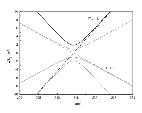
Figure 1: Energy of the dressed levels in the magnetic quadrupole trap described in the paper, plotted along the radial coordinate, in the vicinity of the potential minimum at $\rho=r_{0}$. The five dressed sub levels for a $F=2$ spin state are plotted, as well as two bare states for comparison (bare state $m_{F}=-1$ is shown dashed and $m_{F}=2$ dash-dotted). The ring trap we discuss in this paper is based on the upper dressed potential $m_{F}=F=2$, for the radial trapping (bold solid line). Values for the field gradient, and rf and Rabi frequencies are given in Table 1.

Here, $m_{F}=F=2$ for ⁸⁷Rb and $V_{B}(\mathbf{r})=g_{L}\mu_{B}B(\mathbf{r})$ is the potential created by the magnetic trap alone for $F=2,m_{F}=1$, where $g_{L}$ is the Landé factor and $\mu_{B}$ the Bohr magneton. The potential at the bottom of this magnetic trap is $V_{\rm min}=g_{L}\mu_{B}B_{0}=\hbar\omega_{0}$. The detuning $\Delta=\omega_{\rm rf}-\omega_{0}$ is the difference between the rf applied frequency and the resonant frequency at the magnetic potential minimum, and $\Omega=g_{L}\mu_{B}B_{\rm rf}/2\hbar$ is the Rabi frequency of rf coupling note1 . The potential minimum of this new trap sits on an iso-$B$ surface, as $V_{d}(\mathbf{r})$ has a minimum for $V_{B}(\mathbf{r})=\hbar\Delta$, that is on the surface defined by $g_{L}\mu_{B}B(\mathbf{r})=\hbar\Delta$. In the following, we will concentrate on the case of a quadrupolar trap with $z$ as symmetry axis note2 . Note that in this case the magnetic field in the center is zero, so that $\Delta=\omega_{\rm rf}$ and $V_{\rm min}=0$. Let $b^{\prime}$ be the field gradient in the radial direction, and let us define $\alpha$ as $\alpha=g_{L}\mu_{B}b^{\prime}/\hbar$. In this case, an atom is in a dressed state with potential

$$V_{d}(\rho,z)=F\hbar\left((\alpha\sqrt{\rho^{2}+4z^{2}}-\Delta)^{2}+\Omega^{2}\right)^{1/2}$$ (2)

and the relevant iso-$B$ surface is an ellipsoid of equation $\rho^{2}+4z^{2}=r_{0}^{2}$, where $\rho^{2}=x^{2}+y^{2}$ and the radius $r_{0}$ is related to $\Delta$ through $r_{0}=\Delta/\alpha$, typically much greater than a micrometer. In the presence of gravity, the atoms fall to the bottom of this shell: the resulting trapped cloud is in a quasi 2D geometry. This situation was recently demonstrated experimentally in a Ioffe-Pritchard type trap Colombe04 . It was also used in an atom chip experiment for producing a double well potential Schumm05 .

Let us now add an optical standing wave to this egg shell trap, along the vertical $z$ direction, blue detuned by $\delta>0$ with respect to an atomic dipolar transition note3 and with identical linear polarization for the two laser beams (Figure 4). The light shift creates a periodic potential of period $\lambda/2$ where $\lambda$ is the light wavelength. Along $z$, the atoms are then confined in a series of parallel planes. In a given plane, their altitude is fixed to $z=z_{0}$ better than a fraction of $\lambda$. As a result, if they also experience the adiabatic rf potential in a quadrupole trap, the atoms sit on a circle, the intersection of that plane and the iso-B ellipsoid, defined by $\rho=R$ of radius $R=\sqrt{r_{0}^{2}-4z_{0}^{2}}$ much greater than $\lambda$ (Figure 2). This is the circular trap we are interested in.

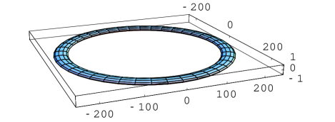
Figure 2: (Color online) A view of the ring trap. An iso-potential surface is plotted for the parameters of Table 1, in the harmonic approximation. The length unit is $1~{}\mu$m. The vertical direction was amplified 10 times for clarity. The overall trap shape is that of a Saturnian ring.

The total potential for the atoms may be written as

$$V(\rho,z)=V_{d}(\rho,z)+U_{0}(1-\cos(2kz))\,e^{-2\rho^{2}/w^{2}}+mgz$$ (3)

where $k=2\pi/\lambda$ is the wave vector of one of the counter-propagating light beams, $U_{0}$ is the mean light shift of the standing wave on axis and $w$ the $1/\sqrt{e}$ diameter. Gravity was taken into account by the last term. $U_{0}$ is assumed to be large enough for the tunnel effect between successive planes to be negligible (see section IV). Note that the potential does not depend on the azimuthal angle $\theta$. For the $D2$ transition of ⁸⁷Rb, the expression for $U_{0}$ is

$$U_{0}=\frac{2}{3}\frac{\Gamma}{\delta}\frac{2P}{8\pi w^{2}I_{s}}\,\hbar\Gamma$$ (4)

where $\Gamma=2\pi\times 5.89$ MHz is the natural linewidth of the transition, $P$ the total laser power and $I_{s}=1.6$ mW/cm² is the saturation intensity. The factor $2/3$ accounts for the transition coefficients of the $D2$ line for a linear polarization.

Let us focus on the plane situated around $z=0$, so that $z_{0}=0$ and $R=r_{0}$. In principle, the trapping potential mixes the radial ($\rho$) and axial ($z$) coordinates. However, the constraints on $\rho$ and $z$ are such that the potential may be written to a good approximation as a sum of independent potentials $V_{\rho}(\rho)$ and $V_{z}(z)$ for the radial and axial coordinates respectively. Indeed, due to the presence of the standing wave, $|z|$ is restricted to values less than $\lambda/4$, typically 100 nm. This is small as compared to $d=\Omega/\alpha$, the length scale associated with the rf coupling [see Eq. (2)] which is on the order of a few micrometers. The $z$ dependence may thus be omitted in $V_{d}$. In the same way, $\rho$ extends over $d$ which is small as compared to the waist $w$. This waist should be chosen of the order of the radius $r_{0}$ (see section V), that is a few hundred micrometers, and then $\rho$ may simply be replaced by $r_{0}$ in the expression of the light shift. Within these assumptions, the single particle hamiltonian becomes separable in $\rho$ and $z$ and one can calculate independently oscillation frequencies along $z$ and $\rho$ around $z=0$ and $\rho=r_{0}$ for an atom of mass $m$:

$$\omega_{\rho} = \alpha\sqrt{F\frac{\hbar}{m\Omega}}$$ (5)

$$\omega_{z} = \frac{2\pi}{\lambda}\sqrt{\frac{4U_{0}}{m}}\,e^{-r_{0}^{2}/w^{2}}.$$ (6)

Thus the total potential for the atoms, Eq. (3), can be written approximately as

$$V(\rho,z)=F\hbar\Omega+\frac{1}{2}m\omega_{\rho}^{2}(\rho-r_{0})^{2}+\frac{1}{2}m\omega_{z}^{2}z^{2},$$ (7)

which is illustrated for an iso-potential surface in Figure 2. (In Eq.(7) we neglect a slight vertical shift in the position of the minimum of the potential due to gravity. This does not significantly affect the vibrational frequency for typical parameters given below.) For the parameters proposed in Table 1 and used in the rest of the paper, we obtain oscillation frequencies of $\omega_{\rho}/2\pi=1.1$ kHz and $\omega_{z}/2\pi=43$ kHz, with a ring diameter of $430~{}\mu$m.

III Conditions for reaching the low dimensional regime

An interesting feature of this ring trap is its high oscillation frequency in the transverse direction. It is thus relevant to raise the question of dimensionality of a degenerate gas confined in this trap. This question has acquired a growing interest in the last 5 years, and is related for instance to the creation of anyons Paredes01 or the fermionization of the excitations in the bosonic cloud Girardeau60 . Already in a 3D elongated condensate, the coherence properties are affected by the geometry Petrov ; Richard03 ; Hugbart05 ; Hellweg03 . To estimate in which regime (1D, 2D or 3D) the gas has to be considered, we compare the chemical potential, calculated in the Thomas Fermi approximation under a given dimensionality assumption, to the trapping oscillation frequencies. The three regimes (3D, 2D or 1D) correspond respectively to $\mu>\hbar\omega_{z}$, $\hbar\omega_{\rho}<\mu<\hbar\omega_{z}$ and $\mu<\hbar\omega_{\rho}$. The cross-over between one regime and another may be given in terms of atom number in the trap. Detailed calculations of the chemical potential in the different regimes are given in appendix A.

Let us first estimate the 3D Thomas-Fermi chemical potential. It can be calculated from the normalization of the condensate wave function in the Thomas-Fermi approximation. The 3D interaction strength is $g_{3D}=4\pi\hbar^{2}a/m$, $a=5.4$ nm being the 3D scattering length. In the harmonic approximation for the toroidal potential, where Eq.(7) is valid, the chemical potential is given by the formula of Eq.(18) note4 :

$$\mu_{3D}=\hbar\bar{\omega}\sqrt{\displaystyle\frac{2Na}{\pi r_{0}}}$$ (8)

where $\bar{\omega}=\sqrt{\omega_{\rho}\omega_{z}}$ is the geometric mean of the oscillation frequencies and $N$ the atom number. This expression is meaningful if the gas is 3D, that is if $\mu_{3D}>\hbar\omega_{z}$. In terms of atom number, it can be expressed as $N>\frac{\pi r_{0}}{2a}\frac{\omega_{z}}{\omega_{\rho}}$, that is $N>2.4\times 10^{6}$ for the choice of the parameters given in Table 1. This number is sufficiently high that it is feasible to have a condensate which is at least in a two-dimensional regime, without any difficulty in imaging it. With $10^{5}$ atoms for instance, the chemical potential corresponds to $\mu_{3D}/h=8.9$ kHz, which is below the highest oscillation frequency of 43 kHz. The total energy per atom does not allow us to populate transverse ($z$) excitations, and the vertical degree of freedom is frozen. Such a degenerate gas would thus be at least in the 2D regime and the chemical potential has to be recalculated within a 2D hypothesis.

In the 2D case, the interaction strength is modified and reads $g_{2D}=g_{3D}/(\sqrt{2\pi}l_{z})=2\sqrt{2\pi}\hbar^{2}a/(ml_{z})$ where $l_{z}=\sqrt{\hbar/(m\omega_{z})}$ is the size of the ground state of the harmonic oscillator in the frozen direction ShlyapnikovQGLD . Again, the chemical potential in 2D is deduced from normalization of the integrated density to the atom number in the Thomas-Fermi regime, Eq.(21):

$$\mu_{2D}=\hbar\bar{\omega}\left(\frac{\omega_{\rho}}{\omega_{z}}\right)^{1/6}\left(\frac{3Na}{4\sqrt{\pi}r_{0}}\right)^{2/3}.$$ (9)

The gas would be in the 1D regime if the 2D chemical potential is of the order of, or less than the radial oscillation frequency $\omega_{\rho}$. This corresponds to an atom number $N<\frac{4\sqrt{\pi}r_{0}}{3a}\sqrt{\frac{\omega_{\rho}}{\omega_{z}}}$, that is $N<1.5\times 10^{4}$ for the proposed parameters. A uniform 1D gas of density $n_{1}=N/(2\pi r_{0})$ would have an interaction strength $g_{1D}=g_{3D}/(2\pi l_{z}l_{\rho})=2\hbar^{2}a/(ml_{z}l_{\rho})$ ShlyapnikovQGLD with $l_{\rho}=\sqrt{\hbar/(m\omega_{\rho})}$, and a chemical potential $\mu_{1D}$ in the trap, with

$$\mu_{1D}=\hbar\bar{\omega}\frac{Na}{\pi r_{0}}.$$ (10)

Again, this expression is valid if the kinetic energy is negligible as compared to the mean-field energy. However, even if this is the case, longitudinal excited states (along the ring) are likely to be populated as the excitation frequency is only of the order of 1 mHz. With such a 1D system, the gas could be in the Tonks-Girardeau regime Girardeau60 ; Tonks if the parameter $\gamma=mg_{1D}/(\hbar^{2}n_{1})$ is much larger than 1. For our parameters, this would correspond to very few atoms, i.e. much less than the $\gamma=1$ limit of 850 atoms. With a larger atom number (a few thousand), we should instead have a quasi-condensate with a fluctuating phase ShlyapnikovQGLD .

In conclusion to this section, let us stress that an atomic cloud confined in the ring trap proposed in this paper would easily be in the 2D regime, the vertical ($z$) degree of freedom being frozen. With the parameters of Table 1, it would be true for an atom number between $1.5\times 10^{4}$ and $2.4\times 10^{6}$. The 1D regime is achievable with a smaller number of atoms, but the Tonks-Girardeau regime would require a few hundred atoms only, and the detection of the atomic cloud would then be an issue.

IV Lifetime in the ring trap

In the ring trap, the lifetime may be limited by several processes, apart from the collisions with the background gas. In this section, we discuss these losses for the ground-state or for thermal atoms.

First, as the atoms are confined in a rf-dressed state, they may undergo non-adiabatic Landau-Zener transitions to an untrapped spin state due to motional coupling. This will happen along the radial axis, where the potential changes more rapidly. The transition rate $\Gamma_{LZ}$ may be estimated by averaging over the velocity distribution the transition probabilities $P_{LZ}$ for a given radial velocity $v_{\rho}$ Vitanov97 :

$$P_{LZ}(v_{\rho})=1-[1-\exp(-\frac{\pi\Omega^{2}}{2\alpha v_{\rho}})]^{2F}\simeq 2Fe^{-\frac{\pi\Omega^{2}}{2\alpha v_{\rho}}}$$ (11)

The loss rate to other spin states is deduced from this transition probability by multiplying by twice the radial oscillation frequency, as the transition may occur at each crossing. With the parameters given above, the transition rate is limited to $\Gamma_{LZ}=\langle P_{LZ}(v_{\rho})\rangle\omega_{\rho}/\pi\simeq 0.075$ s^-1 for a thermal cloud of temperature $3~{}\mu$K. For atoms in the vibrational ground-state of the dressed potential, the approach of Ref. Zobay04 and its Eq.(10), may be generalized to a $F$ spin state as done in Ref. Vitanov97 . The transition rate is then approximately $\Gamma_{gs}\simeq 2\,(F\omega_{\rho}/\pi)\exp[-\pi\Omega/(2\sqrt{2}\omega_{\rho})]$. This leakage is negligible for the parameters of Table 1.

Second, we shall consider the issue of tunneling of the atoms between the vertical lattice sites. For a horizontal lattice – that is, without the effect of gravity – the tunneling amplitude per atom $J$ is related to the lattice depth. In the tight binding limit, where the lattice depth $V_{0}=2U_{0}\,e^{-2r_{0}^{2}/w^{2}}$ is much higher than the recoil energy $E_{R}=h^{2}/(2m\lambda^{2})$, $J$ scales approximately as $(V_{0}/E_{R})^{1.05}e^{-2.12\sqrt{V_{0}/E_{R}}}$ ReyPhD . In the case discussed here, $V_{0}=32~{}E_{R}$ and the tunneling rate $J/h$ is only 1.3 Hz. This rate is even smaller when gravity is taken into account, as it splits the degeneracy between neighbouring ground states by a value $mg\lambda/2h=1/\tau_{B}=822$ Hz ($\tau_{B}$ is the Bloch period). For the given lattice depth, we are deeply in the adiabatic limit and the atoms remain in the ground state band and experience Bloch oscillations: if one starts with atoms in a single lattice well (a Wannier state), after a Bloch period they are all back in the same well. Moreover, the amplitude of these Bloch oscillations in space is very small (2 nm). Only finite size effects, lattice imperfections or excitations to the first excited band would prevent the exact return to initial condition. Tunneling should not be an issue for this trap, at least for the parameters mentioned above.

Finally, photon scattering may lead to heating and trap losses. These processes are quite small for blue detuned lattice light, because the atoms only significantly scatter photons when they leave the very center of a lattice well. In a given well, the scattering rate per atom is related to the cloud spreading $\langle z^{2}\rangle$ and can be expressed as

$$\Gamma_{\rm sc}=\frac{\Gamma}{2}\frac{m\omega_{z}^{2}\langle z^{2}\rangle}{\hbar\delta}.$$ (12)

This simplifies to $\Gamma_{\rm sc}=\Gamma\,\omega_{z}/4\delta$ in the ground state of the vertical motion, and to $\Gamma_{\rm sc}=\Gamma\,k_{B}T/2\hbar\delta$ for a thermal gas. The corresponding calculated values are $\Gamma_{\rm sc}=0.08~{}$s^-1 for the ground-state and $\Gamma_{\rm sc}=0.25~{}$s^-1 for a thermal gas at $3~{}\mu$K, or equivalently a heating rate of 30 nK/s and 90 nK/s respectively Grimm00 .

V Choice of the experimental parameters

In this section we propose a strategy for an optimal choice of the laser, magnetic field and rf field parameters. A correct choice of these experimental parameters should allow one to have a ring trap as large as possible, with high vertical and transverse oscillation frequencies, and reasonable values for magnetic, RF and optical fields, while minimizing the spontaneous photon scattering rate and tunneling between neighbouring wells. With this objective, it appears that the magnetic gradient and the laser power should be chosen as large as possible: only technical issues will limit this choice. We thus fix these parameters to values easily obtainable experimentally, that is a laser power of 0.5 W, available for instance from a Titanium Sapphire laser, and a magnetic gradient $b^{\prime}=150$ G/cm, corresponding to a gradient of 300 G/cm in the axis of the quadrupole coils, already realized in a previous experiment Colombe03 . $b^{\prime}$ is related directly to the parameter $\alpha$ introduced in section II.

An important remark concerns the choice of the beam waist $w$, for a desired ring radius $r_{0}$. There is an optimal choice, maximizing the lattice depth and consequently the vertical oscillation frequency. The waist should be equal to $w=\sqrt{2}\,r_{0}$, the $\sqrt{2}$ coefficient corresponding to the maximum of the function $\frac{1}{x}e^{-1/x^{2}}$, as can be deduced from Eq.(6). This fixes the relation between the light shift in the beam centre $U_{0}$ and the lattice depth: $V_{0}=2U_{0}/e$.

Once these values are fixed, we impose constraints on the possible losses or heating rates discussed in section IV, that is on the tunneling rate $J$, the scattering rate $\Gamma_{\rm sc}$, and the Landau-Zener transition rate $\Gamma_{LZ}$. We set these rates respectively to a given $J_{0}$, to some small fraction $\varepsilon$ of the natural linewidth ($\Gamma_{\rm sc}=\varepsilon\Gamma$) and to $\Gamma_{LZ}=\gamma$. Now, the choice of $J$ imposes the standing wave depth $V_{0}$ (see section IV), as well as the vertical oscillation frequency $\omega_{z}$, directly related to $V_{0}$ and $E_{R}$ through $\hbar\omega_{z}=2\sqrt{V_{0}E_{R}}$. This in turn gives the detuning to be chosen for limiting the photon scattering rate in the ground state to $\varepsilon\Gamma$: $\delta=\omega_{z}/4\varepsilon$ (see section IV). The light shift $U_{0}$ is known from its fixed relation with $V_{0}$, and as the laser power $P$ and the detuning $\delta$ have been chosen, the waist $w$ can be deduced from the knowledge of $U_{0}$. From $w$ one gets $r_{0}=w/\sqrt{2}$ and the rf detuning $\Delta=\alpha r_{0}$. The only remaining parameter is then the rf Rabi frequency $\Omega$, which is chosen to fit the desired value of $\gamma$.

We applied this procedure to desired values of $J/h=1$ Hz, $\Gamma_{\rm sc}=0.1$ s^-1 and $\gamma=0.1$ s^-1 at $3~{}\mu$K to obtain the typical parameter values suggested in Table 1.

Parameter	Value
Laser power $P$	0.5 W
Laser wavelength $\lambda$	771 nm
Beam waist $w$	$300~{}\mu$m
rf Rabi frequency $\Omega/2\pi$	20 kHz
rf frequency $\Delta/2\pi$	2250 kHz
Magnetic field gradient $b^{\prime}$	150 G/cm

Table 1: Typical set of parameters for the realization of the ring trap. The laser used for the standing wave may be a Titanium Sapphire laser.

VI Loading

A condensate in the proposed ring trap would cover quite a small volume spread over a relatively large area, and as a result the method used to load the atoms into the trap needs to be considered carefully. This is because of the mismatch between the starting point, a condensate in a magnetic trap, which may be spheroidal and localised, and the end-point, a condensate in a ring trap which has essentially no overlap with the starting point at all.

There may be several approaches to loading the proposed ring trap. Based on a previous experiment Colombe03 , which used a QUIC trap, our proposed loading method takes place in at least five stages [(i-v) below] and is illustrated in Figure 3. In the following we refer to a BEC for convenience. The steps are the same for a cold atom cloud, but a condensate has an advantage of compactness.

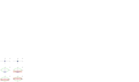
Figure 3: (Color online) Outline illustration of stages in the loading of the ring trap. The $z$-axis is in the vertical direction and we assume a cylindrical symmetry about this axis. In (b-f) the elliptical line indicates the location (in the $y$-$z$ plane) of the rf resonance. In (d-f) the horizontal bands indicate the presence of the standing light wave. Then: (a) We take as the starting point a BEC in a magnetic trap. (b) Shortly after transfer to the dressed rf trap the condensate fills a location around the rf resonance, but is not yet excluded from the trap centre. (c) After rf expansion (stage (ii)) the condensate lies at the bottom of the ‘egg-shell’. (d) The application of the optical standing wave results in a potential which confines the condensate to a couple of potential wells (corrugations). (e) The standing wave is moved upwards and the condensate ring is formed and expanded outwards and upwards. (f) Final position of the condensate ring at maximum radius. All three potentials, magnetic, dressed rf, and optical are required to maintain the ring.

(i) Dressed trap loading: Starting with the magnetic trap, Fig.3(a), the condensate is first transferred to the field-dressed atom trap (ZG-trap) by an established loading procedure Zobay01 ; Colombe04 in which a rf field is steadily increased in intensity at a fixed, negative, detuning (relative to the magnetic trap centre) and subsequently ramped up in frequency to positive detuning (see Fig.3(b)). This accomplishes a transfer to field-dressed potentials, like those in Eq. (2), which are subsequently expanded outwards from the trap centre as seen in Fig.3(c). (This rf expansion is discussed further in (ii), below.)

In the resulting trap the condensate lies in an electromagnetic potential which confines it to the surface of an ellipsoid, or egg-shell as in section II. This surface is represented by the ellipse in Fig.3(b-f). However, gravity, and the absence of the optical potential, ensures that the condensate occupies just the lower part of the ellipsoid surface, when the ellipsoid is sufficiently large, and as seen in Fig.3(c). As mentioned in section II the egg-shell is defined, for a particular rf frequency, by the surface of resonance between the magnetic sub-levels and the rf. Thus the size of the ellipsoid, or egg-shell, depends on the rf frequency; so as the rf frequency is increased, the part of the condensate at the the bottom of the egg shell moves downwards and becomes flatter. This is the rf expansion phase and is represented by the transition from Fig.3(b) to Fig.3(c).

(ii) RF expansion: During the rf expansion the pendulum frequency reduces considerably. Numerical simulations of this kind of expansion, as part of a loading process, were carried out in Ref. Zobay04 . To give an example for the current ring trap, we may consider $10^{5}$ atoms in the dressed trap. We will also have an underlying magnetic trap with the parameters given in section V and a rf intensity leading to the same dressed trapping frequency $\omega_{trans}=2\pi\times 2.26$ kHz at the final rf frequency. With the rf thus chosen the condensate would be at a distance of $z_{0}=$107 $\mu$m below the magnetic trap centre, and the final horizontal oscillation frequency (given in Appendix B) is $\omega_{1,2}=\sqrt{g/4z_{0}}$ with a value of approximately 24 Hz. Thus, since this is the lowest horizontal frequency during expansion, the timescale for the expansion needs to be considerably longer than the corresponding characteristic time-scale $1/24\sim 42$ ms. If it is not, there will be lateral excitations. Since the condition for adiabaticity is that $\dot{\omega_{1,2}}\ll\omega_{1,2}^{2}$ Zobay04 , we can make an estimate for the required expansion time by solving the equation $\dot{\omega_{1,2}}=-\epsilon\omega_{1,2}^{2}$, where $\epsilon$ represents an amount of non-adiabaticity that can be tolerated. Thus an overestimate of the expansion time is $1/(\epsilon\omega_{1,2})$ if the value of $\omega_{1,2}$ is the final horizontal oscillation frequency. (This neglects the initial horizontal oscillation frequency in comparison with the final value.) Then a tolerance of $\epsilon\sim 1\%$ leads to an expansion time of 0.7 s.

The condensate would thus be flattened. The aim is to flatten it sufficiently to be able to load it as efficiently as possible into a single corrugation of the optical potential created by the blue-detuned standing wave. The best case would be if the condensate could be flattened to match its width in the optical potential. In practice we would expect difficulties with this step. Physical constraints on the size of the magnetic coils and the fields they produce mean that it can be hard to make a condensate with many atoms sufficiently thin, without retaining some of the curvature of the egg-shell. Thus a curved standing wave would be ideal, since it would match better the shape of the curved condensate. However, from the experimental point-of-view this would be complicated to set up and adjust. Thus we will consider a planar standing wave in what follows. In this case it means that when the standing wave is applied the condensate may be sliced into a number of rings and a central disc. Fig.3(d) shows a disc and just one such ring as an example. Each ring would be formed from condensate collected within a distance given by the well separation of the optical potential (i.e. within a range of $\lambda/2$).

Since the aim is to study the condensate properties in one of the rings, it is important to estimate the fraction of condensate that might be lost from the principal ring in the loading process. An estimate can be formed by considering the Thomas-Fermi approximation for the condensate density in the egg-shell trap. A simple model of the trap consists of a radial potential $m\omega_{trans}{{}^{2}}(r-R)^{2}/2$ representing the shell with a local curvature $R$, a local oscillation frequency $\omega_{trans}$ in the ‘shell’, and a simplified gravitational potential (see Appendix B).

Again, as a numerical example, we consider $10^{5}$ atoms in the dressed trap with the rf at its final value so that the condensate lies at a distance of 107 $\mu$m below the magnetic trap centre. Then the Thomas-Fermi solution, see Appendix B, gives a condensate with a maximum total thickness of 0.60 $\mu$m, a horizontal full width of 56 $\mu$m and a height (from the resonance point) of 0.92 $\mu$m. The height and maximum thickness are in the region of twice the proposed optical well separation of $\lambda/2\sim 0.39~{}\mu$m. The number of atoms caught in the loading process can be estimated by integrating the Thomas-Fermi solution over a vertical distance of $\lambda/2$. In this example we numerically find that at best 60% of atoms could be loaded into a single well, and roughly 3 other rings are populated to a lesser extent.

In this example the condensate is already close to a two-dimensional regime. If we increase the displacement of the condensate, by increasing the rf frequency and keeping other parameters constant, we find that there is a slight reduction in thickness and height, but even at a displacement of 200 $\mu$m the thickness is 0.53 $\mu$m with the other parameters as given. Increasing the rf in this way also has side-effects, such as a reduction in the lateral oscillation frequency $\omega_{1,2}=\sqrt{g/z_{0}}/2$ and consequent increased loading time. We note that if curvature were more of a problem than thickness, the situation could be improved by the application of red-detuned light to attract the atoms, temporarily, into the centre. Such a horizontal confinement may cause some increase in (vertical) thickness, for a given number of atoms, and so there may still have to be a trade-off between the curvature of the condensate and its thickness. An increase in either thickness, or curvature, could result in atoms being spread amongst several other optical wells when the standing wave is applied.

(iii) Improve magnetic trap geometry: As soon as the condensate has moved away from the centre of the magnetic trap, it is advantageous to improve the magnetic configuration by removing any bias fields needed in the original magnetic trap. For example, with a QUIC trap configuration we can achieve a quadrupole field by turning off the Ioffe coil. This will result in a circularly symmetric ring trap at the final stage, and by doing this while the condensate is still fairly localised, we again reduce the demands of adiabaticity on the time-scales of the system. (As soon as the condensate has moved away from the centre of the trap there is no longer any need to worry about any Majorana transitions.)

(iv) Application of optical potential: Now the blue-detuned standing wave can be applied and as many atoms as possible are trapped in a single well, or corrugation, of the optical potential. Figure 3(d) shows a case where a single other well is also populated. The light is switched on relatively slowly so as not to cause any excitation of the condensate.

We note that the option exists, at this point in the loading sequence, to remove unwanted atoms from some of the optical wells by applying an rf ‘scalpel’. However, this procedure would require an adiabatic unloading and reloading of the dressed rf trap, which can be done, but adds to the overall loading time.

(v) Ring expansion: The final stage of the loading process is to form the condensate ring by changing the vertical position of the blue-detuned potential well relative to the rf resonance point, or egg-shell. If we consider the standing wave as comprised of two traveling waves, this can be done by simply changing the phase of one of the traveling wave components. When this is done the standing wave pattern can be moved upwards. As this happens, the confinement to the egg-shell of the rf trap ensures the formation of a ring of condensate. The ring expands outwards as it is raised upwards (Fig. 3(e)). During this expansion the orientation of the softer rf trapping changes from the vertical to the horizontal and the condensate will adopt the shape of a Saturnian ring which becomes narrower when the rf trapping is fully in the horizontal direction.

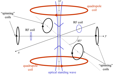
Figure 4: (Color online) Coils and laser configuration for producing and exciting the ring trap. The trap is the combination of a vertical light standing wave (blue beam on the figure) and an egg shell rf trap (see section II). This egg shell trap relies on a magnetic field gradient (produced by the quadrupole coils) and rf coupling between Zeeman sub levels (two rf coils in quadrature as described in section VI). The additional “spinning” coils could be used for exciting the rotation of the atoms inside the ring trap (see section VII).

Clearly, the ring reaches a point of maximum circular radius when its centre is at the centre of the quadrupole trap. However, we note that whilst the magnitude of the magnetic field remains constant, the orientation of the magnetic field changes as the ring is raised. Since the orientation of the magnetic field is important in the orientation of the antenna (see note note1 ) this would necessitate switching between different antennas at about the half-way point. A problem that then emerges is that the rf trapping becomes asymmetrical as soon as the ring starts to expand, and consequently, until the switching occurs, the ring is squeezed more tightly in one direction. A better solution to the problem of the orientation of the antenna avoids any switching by utilizing a rf magnetic field rotating in the horizontal plane. This field can be generated by two rf coils at right angles to each other (Figure 4). When the condensate is at the bottom of the egg-shell potential, the magnetic field is basically vertical and provided the rf field is rotating in the correct direction the rf dressed trapping is fully effective. When the condensate is at the horizontal extremum of the egg-shell, i.e. forming a ring, the magnetic field is horizontal and at each point on the ring the rotating field always has one ineffective component and an effective component perpendicular to the local static magnetic field. As a result the rf trapping is uniform around the ring without needing to switch. The reduced effective amplitude can be compensated by an increase in rf power as the ring expanded to its full radius.

Finally, we note that instead of raising the standing wave pattern, the ring could also be expanded by further increase of the rf detuning. This would force the ring outwards at the same vertical position, i.e. at 107 $\mu$m below the magnetic trap centre in the example given.

VII Conclusion

In this paper we have seen how a ring trap for cold atoms can be made from a combination of magnetic, rf and optical fields. It is the combination of these fields which makes possible a trap with sufficient tightness that it could hold 2D and even 1D condensates. Many of the physical parameters of the trap are the result of practical compromises which have been tested in this paper. For example, the leakage in the optical trap component is traded off against practical laser power and reduced photon scattering. The leakage of the rf trapping component is traded off against its tightness. The number of atoms should be sufficiently high that it can be easily imaged. Additional calculations have shown that a small tilting of the trap will not adversely affect it. The ring trap also has to have a loading scheme and a possibility has been presented in this paper which involves careful orientation of the rf antennae to maintain rf trapping as the atom ring is formed. A set of feasible parameters for the trap has been presented which still leaves room for later optimisation and yet would allow the demonstration of the ring trap and low-dimensional effects.

Once the atom ring is created it could be excited, or manipulated, with the application of a periodic perturbation. Optical ‘paddles’ can be used to good effect (see e.g. Ref. Madison99 ), but another way to do this would be with a rotating deformation of the ring. This can be achieved with the magnetic field from two pairs of coils, each of which is in an anti-Helmholtz configuration with its axis oriented in the horizontal plane and at a 45^∘ angle to the axis of the other pair (Figure 4). Each pair of coils can perturb the circular shape of the ring trap on its own. It can be shown that one pair of these coils results in an ellipse with a difference in radii of

$$\delta r_{0}\simeq\frac{3}{2}\frac{\delta b^{\prime}}{b^{\prime}}r_{0}\,,$$ (13)

where $\delta b^{\prime}$ is the magnetic field gradient produced along the axis of the coils. By applying a time-dependent function to the current of the pairs of coils the elliptical trap can be continuously rotated. This may initiate a collective movement, or excitation, of the trapped cloud or condensate as has been explored in some theoretical papers Javanainen98 ; Salasnich99 ; Brand01 ; Javanainen01 ; Nugent03 ; Bhattacherjee04 . As well as studying persistent currents the trap makes an interesting topology to study solitons in three and less dimensions Brand01 . Furthermore, it would be possible to study the implosion of an atom ring, and the effect of repulsive interactions, by switching off the rf coupling. The magnetic field would then cause some components of the BEC to be expelled, and some to be drawn into the centre where the atom ring would be turned inside-out after some effect of the interactions.

As mentioned in the Introduction the set-up for this ring trap also makes it possible to have multiple ring traps by utilizing the periodicity of the standing wave. Interferences between multiple rings could be obtained either by releasing the vertical confinement alone – and maintaining the rf shell – or by releasing both vertical and horizontal confinement to allow a full expansion of the degenerate gas. It would also make it possible to image vortices and phase fluctuations in a 2D ring (similarly to the imaging of sheets in Ref. Dalibard05 ). In the same way the sudden loss of just the vertical confinement can create some interesting dynamics in the shell as the rings overlap.

In this trap the rf dressed-state trapping and the tight optical confinement can be adjusted independently of each other. Thus our ability to convert between a ring trap and a pancake trap (without the rf) allows a study of the interplay between persistent currents and vortices as the restricted geometry of the trap is changed, as well as an exploration of how superfluidity is connected to BEC, and other quantum gases BlochKavoulakis , during such a geometric crossover.

Since this paper was submitted we have become aware of two other proposals for smaller ring traps Lesanovsky06 ; Fernholz05 which utilize dressed-state rf trapping in different ways.

We acknowledge fruitful discussions with Rudi Grimm. This work is supported by the Région Ile-de-France (contract number E1213) and by the European Community through the Research Training Network “FASTNet” under contract No. HPRN-CT-2002-00304 and Marie Curie Training Network “Atom Chips” under contract No. MRTN-CT-2003-505032. Laboratoire de physique des lasers is UMR 7538 of CNRS and Paris 13 University. The LPL group is a member of the Institut Francilien de Recherche sur les Atomes Froids. B. M. Garraway is a visiting professor at Paris 13 University.

Appendix A Thomas-Fermi solution for the ring trap in 3D, 2D and 1D

In this section, we give a detailed calculation of the chemical potential in the Thomas-Fermi approximation for the ring trap in the harmonic approximation, depending on the dimension. Let us first consider the 3D case. The 3D density is related to the ring trapping potential (7) through

$$n_{3D}(\rho,z)=\frac{\mu_{3D}-\frac{1}{2}m\omega_{\rho}^{2}(\rho-r_{0})^{2}-\frac{1}{2}m\omega_{z}^{2}z^{2}}{g_{3D}}$$ (14)

in the region of space where this quantity is positive. This region is defined by $(\rho-r_{0})^{2}/R_{\rho}^{2}+z^{2}/R_{z}^{2}<1$, where $R_{\rho}$ and $R_{z}$ are related to $\mu_{3D}$ through $\mu_{3D}=\frac{1}{2}m\omega_{\rho}^{2}R_{\rho}^{2}=\frac{1}{2}m\omega_{z}^{2}R_{z}^{2}$. Due to the trap rotational invariance, the atomic density does not depend on the polar angle $\theta$. The chemical potential is given by normalization of the integrated density to the atom number:

$$N=2\pi\int_{-R_{z}}^{R_{z}}\!\!\!dz\int_{r_{0}-R_{\rho}\sqrt{1-\frac{z^{2}}{R_{z}^{2}}}}^{r_{0}+R_{\rho}\sqrt{1-\frac{z^{2}}{R_{z}^{2}}}}\rho\,d\rho\,n_{3D}(\rho,z)$$ (15)

or, after a substitution $u=(\rho-r_{0})/R_{\rho}$, $v=z/R_{z}$

$$\frac{Ng_{3D}}{\mu_{3D}}=2\pi r_{0}R_{z}R_{\rho}\int_{-1}^{1}\!\!\!dv\int_{-\sqrt{1-v^{2}}}^{+\sqrt{1-v^{2}}}\!\!\!\!du\,(1+\frac{R_{\rho}}{r_{0}}u)(1-v^{2}-u^{2})$$ (16)

The term in $R_{\rho}/r_{0}$ cancels after integration over $u$ because of parity, while the leading term is doubled. After integration, one finds

$$Ng_{3D}=\pi^{2}r_{0}R_{\rho}R_{z}\mu_{3D}.$$ (17)

It leads to the following expression for the chemical potential for a degenerate cloud confined in the ring in the 3D regime:

$$\mu_{3D}=\hbar\bar{\omega}\sqrt{\displaystyle\frac{2Na}{\pi r_{0}}}.$$ (18)

Here, we have used the expressions for $R_{\rho}$ and $R_{z}$ given above, the 3D interaction coupling constant $g_{3D}=4\pi\hbar^{2}a/m$, and the geometric mean of the oscillation frequencies $\bar{\omega}=\sqrt{\omega_{\rho}\omega_{z}}$.

If now the vertical degree of freedom is frozen, the gas enters the 2D regime. The condensate wave function is the product of the harmonic oscillator ground state along $z$, of size $l_{z}=\sqrt{\hbar/(m\omega_{z})}$, and a 2D wave function in the plane, satisfying a 2D Thomas-Fermi equation. The expression for the chemical potential should be calculated from integration of the 2D density, deduced from this equation in the harmonic approximation:

$$n_{2D}(\rho)=\frac{\mu_{2D}-\frac{1}{2}m\omega_{\rho}^{2}(\rho-r_{0})^{2}}{g_{2D}}$$ (19)

for $\rho$ such that this expression is positive. Here, the 2D coupling constant is given by $g_{2D}=g_{3D}/(\sqrt{2\pi}l_{z})=2\sqrt{2\pi}\hbar^{2}a/(ml_{z})$ ShlyapnikovQGLD . Again, if $R_{\rho}$ is such that $\mu_{2D}=\frac{1}{2}m\omega_{\rho}^{2}R_{\rho}^{2}$, we can write

$$\frac{Ng_{2D}}{\mu_{2D}}=2\pi r_{0}R_{\rho}\int_{-1}^{1}\!\!\!\!du\,(1+\frac{R_{\rho}}{r_{0}}u)(1-u^{2}).$$ (20)

Only the leading term contributes for parity reasons and we have $Ng_{2D}=\frac{8\pi}{3}r_{0}R_{\rho}\mu_{2D}$. Using the relation between $R_{\rho}$ and $\mu_{2D}$ and the expression of the interaction coupling constant, the expression for the chemical potential in the 2D regime reads

$$\mu_{2D}=\hbar\bar{\omega}\left(\frac{\omega_{\rho}}{\omega_{z}}\right)^{1/6}\left(\frac{3Na}{4\sqrt{\pi}r_{0}}\right)^{2/3}.$$ (21)

For a 1D gas, both $z$ and $\rho$ degrees of freedom are frozen, with a respective size $l_{z}$ and $l_{\rho}=\sqrt{\hbar/(m\omega_{\rho})}$. The ground-state has a uniform density along the ring $n_{1D}=N/(2\pi r_{0})$, in the Thomas-Fermi approximation, and we have $g_{1D}n_{1D}=\mu_{1D}$. The interaction coupling constant is given by $g_{1D}=g_{3D}/(2\pi l_{z}l_{\rho})=2\hbar^{2}a/(ml_{z}l_{\rho})$ ShlyapnikovQGLD . We obtain directly the chemical potential from this set of equations, as

$$\mu_{1D}=\hbar\bar{\omega}\frac{Na}{\pi r_{0}}.$$ (22)

Appendix B Thomas-Fermi solution for the tight shell trap

Before the optical potential is applied in the loading process the trap potential is that of a dressed rf shell trap in the presence of gravity which results in the atoms collecting at the bottom of the shell. In order to estimate the capture efficiency when the optical potential is applied we utilize the density in the rf trap from the three-dimensional Thomas-Fermi solution. Thus positive densities satisfy $n(r,\theta)=(\mu-V(r,\theta))/g_{3D}$ where $g_{3D}=4\pi\hbar^{2}a/m$. We then approximate the potential for the atoms, Eq. (3) with $U_{0}=0$, by

$$V(r,\theta)=\frac{1}{2}m\omega_{trans}^{2}(r-R)^{2}+mgR(1-\cos\theta).$$ (23)

This potential assumes a tight binding to a shell with a local radius of curvature $R$. For the ellipsoid geometry of section II this means $R=4z_{0}=2r_{0}$. The shell binding frequency $\omega_{trans}$ also has the value local to the bottom of the shell and is assumed independent of radial distance $r$ and angle $\theta$. This independence is not strictly true because the effective rf amplitude and field gradient vary with angle. For a given effective rf amplitude, and for the ellipsoidal geometry of section II the frequency $\omega_{trans}$ at the bottom of the trap is twice radial rf trapping frequency $\omega_{\rho}$ in the ring [Eq. (5)]. The gravitational sag of the shell is also neglected, and varies with position, but this is expected to be small for realistic parameters.

To find the chemical potential we may use a 3D harmonic approximation since the shell approximation is already a radial harmonic potential and the maximum value for $\theta$, for parameters given, is 0.07 radians, allowing the angular part to be harmonic, too. The angular frequency $\omega_{1,2}$ is the same as the pendulum frequency, i.e. $\omega_{1,2}=\sqrt{g/R}=\sqrt{g/(4z_{0})}$. Thus we may use the standard 3D harmonic result Dalfovo99

$$\mu=\frac{\hbar\tilde{\omega}}{2}\left(\frac{15Na}{a_{0}}\right)^{2/5},$$ (24)

with the geometric mean of the oscillation frequencies $\tilde{\omega}=(\omega_{trans}g/R)^{1/3}$, and $a_{0}=\sqrt{\hbar/m\tilde{\omega}}$. The chemical potential found from all the approximations given above agrees well with a numerical integration and is used, with the Thomas-Fermi solution, to estimate the number of atoms loaded into the optical potential.

References

- (1) D.S. Petrov, G.V. Shlyapnikov, and J.T.M. Walraven, Phys. Rev. Lett. 85, 3745 (2000); ibid. 87, 050404 (2001).
- (2) A. Görlitz, J.M. Vogels, A. E. Leanhardt, C. Raman, T.L. Gustavson, J.R. Abo-Shaeer, A.P. Chikkatur, S. Gupta, S. Inouye, T. Rosenband, and W. Ketterle, Phys. Rev. Lett. 87, 130402 (2001).
- (3) S. Dettmer, D. Hellweg, P. Ryytty, J.J. Arlt, W. Ertmer, K. Sengstock, D.S. Petrov, G.V. Shlyapnikov, H. Kreutzmann, L. Santos, and M. Lewenstein, Phys. Rev. Lett. 87, 160406 (2001).
- (4) S. Richard, F. Gerbier, J. H. Thywissen, M. Hugbart, P. Bouyer, and A. Aspect, Phys. Rev. Lett. 91, 010405 (2003).
- (5) I. Shvarchuck, Ch. Buggle, D.S. Petrov, K. Dieckmann, M. Zielonkowski, M. Kemmann, T.G. Tiecke, W. von Klitzing, G.V. Shlyapnikov, and J.T.M. Walraven, Phys. Rev. Lett. 89, 270404 (2002).
- (6) H. Moritz, T. Stöferle, M. Köhl, and T. Esslinger, Phys. Rev. Lett. 91, 250402 (2003).
- (7) B. Laburthe Tolra, K.M. O’Hara, J.H. Huckans, W.D. Phillips, S.L. Rolston, and J.V. Porto, Phys. Rev. Lett. 92, 190401 (2004).
- (8) B. Paredes, A. Widera, V. Murg, O. Mandel, S. Fölling, I. Cirac, G. V. Shlyapnikov, T. W. Hänsch and I. Bloch, Nature 429, 277-281 (2004).
- (9) J.A. Sauer, M.D. Barrett and M.S. Chapman, Phys. Rev. Lett. 87, 270401 (2001).
- (10) A.S. Arnold and E. Riis, J. Mod. Opt. 49, 959 (2002); A.S. Arnold, J. Phys. B: Adv. Mol. Opt. Phys. 37, L29 (2004).
- (11) S. Wu, W. Rooijakkers, P. Striehl, and M. Prentiss, Phys. Rev. A 70, 013409 (2004).
- (12) S. Gupta, K.W. Murch, K.L. Moore, T.P. Purdy, and D.M. Stamper-Kurn, Phys. Rev. Lett. 95 143201 (2005).
- (13) A.S. Arnold, C.S. Garvie, and E. Riis, Phys. Rev. A 73, 041606 (2006).
- (14) F. Bloch, Phys. Rev. A 7, 2187 (1973); and see G.M. Kavoulakis, Y. Yu, M. Ögren, and S.M. Reimann, eprint cond-mat/0510315, and references therein.
- (15) E.M. Wright, J. Arlt, and K. Dholakia, Phys. Rev. A 63, 013608 (2000).
- (16) A. Hopkins, B. Lev, and H. Mabuchi, Phys. Rev. A 70, 053616 (2004).
- (17) O. Zobay and B.M. Garraway, Phys. Rev. Lett. 86, 1195 (2001).
- (18) O. Zobay and B.M. Garraway, Phys. Rev. A 69, 023605 (2004).
- (19) This expression for is valid if the field is orthogonal to the local static magnetic field; if this is not the case, only its orthogonal component contributes to . See e.g. Yves Colombe, PhD thesis, Université Paris 13 (2004).
- (20) The principle of the circular trap is also valid with other kinds of magnetic traps, in particular Ioffe-Pritchard traps. Depending on the axis chosen for the standing wave, the trap may be elliptical instead of circular.
- (21) Y. Colombe, E. Knyazchyan, O. Morizot, B. Mercier, V. Lorent, and H. Perrin, Europhys. Lett. 67, 593 (2004).
- (22) T. Schumm, S. Hofferberth, L. M. Andersson, S. Wildermuth, S. Groth, I. Bar-Joseph, J. Schmiedmayer and P. Krüger, Nature Physics 1, 57 (2005).
- (23) A red detuned light would also be a possible choice. However, the photon scattering rate would be higher in this case.
- (24) B. Paredes, P. Fedichev, J. I. Cirac, and P. Zoller, Phys. Rev. Lett. 87, 10402 (2001).
- (25) M. D. Girardeau, J. Math. Phys. 1, 516 (1960).
- (26) M. Hugbart, J.A. Retter, F. Gerbier, A.F. Varón, S. Richard, J.H. Thywissen, D. Clément, P. Bouyer, and A. Aspect, Eur. Phys. J. D 35, 155 (2005).
- (27) D. Hellweg, L. Cacciapuoti, M. Kottke, T. Schulte, K. Sengstock, W. Ertmer, and J.J. Arlt, Phys. Rev. Lett. 91, 010406 (2003).
- (28) We neglect here the radius variation, which would give a correction of order .
- (29) See e.g. D. S. Petrov, D. M. Gangardt, and G. V. Shlyapnikov, Low-dimensional trapped gases, in Proceedings of Quantum Gases in Low Dimensions, L. Pricoupenko, H. Perrin, and M. Olshanii eds., Journal de Physique IV 116, p.3 (2004), and references therein. Note that the expression for on p.11 should be corrected by a factor of so that it reads: .
- (30) L. Tonks, Phys. Rev. 50, 955 (1936); M. D. Girardeau, Phys. Rev. 139, B500 (1965); M. Olshanii, Phys. Rev. Lett. 81, 938 (1998).
- (31) N. V. Vitanov and K.-A. Suominen, Phys. Rev. A 56, R4377 (1997).
- (32) A. M. Rey, PhD thesis, University of Maryland (2004).
- (33) R. Grimm, M. Weidemüller, and Yu. B. Ovchinnikov, Adv. At. Mol. Opt. Phys. 42, 95 (2000).
- (34) Y. Colombe, D. Kadio, M. Olshanii, B. Mercier, V. Lorent, and H. Perrin, J. Opt. B: Quantum Semiclass. Opt. 5, S155 (2003).
- (35) K.W. Madison, F. Chevy, W. Wohlleben, and J. Dalibard, Phys. Rev. Lett. 84, 806 (2000).
- (36) J. Javanainen, S.M. Paik, and S.M. Yoo, Phys. Rev. A 58, 580 (1998).
- (37) L. Salasnich, A. Parola, and L. Reatto, Phys. Rev. A 59, 2990 (1999).
- (38) J. Brand and W.P. Reinhardt, J. Phys. B: At. Mol. Opt. Phys. 34, L113 (2001).
- (39) J. Javanainen, Y. Zheng, Phys. Rev. A 63, 063610 (2001).
- (40) E. Nugent, D. McPeake, and J.F. McCann, Phys. Rev. A 68, 063606 (2003).
- (41) A.B. Bhattacherjee, E. Courtade, and E. Arimondo J. Phys. B: At. Mol. Opt. Phys. 37, 4397 (2004).
- (42) S. Stock, Z. Hadzibabic, B. Battelier, M. Cheneau, and J. Dalibard, Phys. Rev. Lett. 95 190403 (2005).
- (43) I. Lesanovsky, T. Schumm, S. Hofferberth, L.M. Andersson, P. Krüger, and J. Schmiedmayer, Phys. Rev. A 73, 033619 (2006).
- (44) T. Fernholz, R. Gerritsma, P. Krüger, and R.J.C. Spreeuw, eprint physics/0512017.
- (45) F. Dalfovo, S. Giorgini, L. P. Pitaevskii, and S. Stringari, Rev. Mod. Phys. 71, 463 (1999).