Multifractal analysis of the long-range correlations in the cardiac dynamics of Drosophila melanogaster

Abstract

Time series of heartbeat activity of humans can exhibit long-range correlations. In this paper we show that such kind of correlations can exist for the heartbeat activity of much simpler species like Drosophila melanogaster. By means of the method of multifractal detrended fluctuation analysis (MFDFA) we calculate fractal spectra $f(\alpha)$ and $h(q)$ and investigate the correlation properties of heartbeat activity of Drosophila with genetic hearth defects for three consequent generations of species. We observe that opposite to the case of humans the time series of the heartbeat activity of healtly Drosophila do not have scaling properties. Time series from flies with genetic defects can be long-range correllated and can have multifractal properties. The fractal heartbeat dynamics of Drosophila is transferred from generation to generation.

1 Introduction

The irregular and complex structure of the time series (ECG) of human heartbeat dynamics is an object of considerable clinical and research interest [1], [2], [3]. This structure is connected not only to the external and internal perturbations but also depends on the synergetic action of muscle and nervous systems which influences the correlation properties of the time series. In many simple systems the correlation function of the measured time series usually decays exponentially with the time. In complex systems the correlations can decay with power law and because no characteristic scale is associated with the power law such systems are called scale-free. Their correlations are called long-range because at large time scales the power law function is always larger than the exponential function. Below we are interested in the presence of long-range correlations in the time series for heartbeat activity of Drosophila melanogaster - the classical object of Genetics. Due to the short reproduction cycle of Drosophila we can investigate the correlation properties of the heartbeat dynamics for three consequent generations. This allows us to study the relation between genetic properties of Drosophila and correlation properties of the time series of its heartbeat activity.

The paper is organized as follows. In Sect. 2 we describe the investigated system, recording of the time series and quantities used for their analysis. The analysis of the obtained fractal spectra is performed in Sect.3 . Some concluding remarcs are summarized in the last section.

2 System and methods

We investigate time series of the heart activity (ECG) of Drosophila melanogaster obtained from mutant flies and wild type controls provided by Bloomington Drosophila Stock Center, U.S.A. We crossed male Dopa decarboxilase (Ddc) mutant (FBgn 0000422 located in chromosome 2, locus 37C1) and female shibire (shi) (FBgn 0003392 located in chromosome 1, locus 13F7-12). The Ddc mutants’ heartbeat rate is about 60 % of the normal one. Ddc codes for an enzyme necessary for the synthesis of four neurotransmitters: norepinephrine, dopamine, octopamine, serotonin, related to learning and memory. The shibire (shi) mutants cause paralysis at high temperature. They code for the protein dynamin, necessary for the endocytosis. Its damaging at high temperature stops the transmission of the impulse through the synapses, causes paralysis, and eliminates the effect of the neurotransmitters on the heart [4]. ECGs were taken from three consequent generations of species. Drosophila heartbeat was recorded optically and digitalized. Optical ECG records were taken at a stage P1 (white puparium) of a Drosophila development when it is both immobile and transparent and the dorsal vessel is easily viewed. The object was placed on a glass slide in a drop of distilled water under a microscope (magnification 350 x). Fluctuation in light intensity due to movement of the dorsal vessel tissue was captured by photocells fitted to the one eyepiece of the microscope. The captured analogue signal was then digitized at 1 kHz sampling rate by data acquisition card and LabVIEW data capturing software supplied by National Instruments. 600000 data points were taken for each sample.

The obtained time series are analysed by the multifractal formalism which is widely used in mathematics, physics, and biology [1], [5], [6], [7], [8]. The investigation is based on the spectrum $h(q)$ of the local Hurst exponent and on the fractal spectrum $f(\alpha)$ [9, 10]. Let us consider a set of points which lies in an $N-$dimensional Cartesian space covered by a grid of $N$-dimensional cubes of edge length $\epsilon$. If for small $\epsilon$ we need $N^{*}(\epsilon)$ cubes to cover our set we can define the spectrum of generalized dimensions

$$D_{q}=\frac{1}{1-q}\lim_{\epsilon\to 0}\frac{\ln I(q,\epsilon)}{\ln(1/\epsilon)},\hskip 14.22636ptI(q,\epsilon)=\sum_{k=1}^{N^{*}(\epsilon)}\mu_{k}^{q},$$ (1)

where $q$ is a continuous index. $\mu_{k}$ is the natural measure, i.e., it is a measure of the frequency with which a typical orbit visits various cubes covering the investigated attracting set of points for the limit case when the length of the orbit goes to infinity (in addition the frequences have to be the same for all initial conditions in the basin of attraction of the attractor except for a set with Lebesque measure $0$). Thus for $\mu_{k}$ we have

$$\mu_{k}=\lim_{T\to\infty}\frac{\xi(c_{k},{\bf x}_{0},T)}{T},$$ (2)

where $\xi$ is the time the orbit originating from ${\bf x}_{0}$ spends in the cube $c_{k}$ in the time interval $0\leq t\leq T$. $D_{0}$ is called capacity of the set and it is not integer for some sets. From (1) by means of the L‘Hospital rule we can easily obtain

$$D_{1}=\lim_{\epsilon\to 0}\frac{\sum_{k=1}^{N^{*}}(\epsilon)\mu_{i}\ln\mu_{i}}{\ln\epsilon}$$ (3)

$D_{1}$ is called also information dimension (as it measures how the information is scaled with $\ln(1/\epsilon)$). In general $D_{0}\geq D_{1}\geq D_{2}\geq\dots$. If $D_{q}$ varies with $q$ the measure, associated with $D_{q}$ is called multifractal measure.

Let a set $S$ be covered with a grid of cubes of unit size $\epsilon$ and $\mu$ is the probability measure on $S$ ($\mu(S)=1$). Let $\mu(c_{k})=\mu_{k}$ where $c_{k}$ denotes again the $k-$th cube. We can assign a singularity measure $\alpha_{k}$ to each cube

$$\mu_{k}=\epsilon^{\alpha_{k}}$$ (4)

For small $\epsilon$ we can make continuous approximation for the number of cubes for which $\alpha_{k}$ is between $\alpha$ and $\alpha+d\alpha$, i.e., we can denote this number as $\rho(\alpha)\epsilon^{-f(\alpha)}d\alpha$. Substituting (4) in the relationship for $I(q,\epsilon)$ and after a transition from a sum over the cubes to an integration over the $\alpha$ we obtain

$$I(q,\epsilon)=\sum_{k=1}^{N^{*}(\epsilon)}\epsilon^{\alpha_{k}q}=\int d\alpha^{*}\rho(\alpha^{*})\epsilon^{-f(\alpha^{*})}\epsilon^{q\alpha^{*}}=$$

$$=\int d\alpha^{*}\rho(\alpha^{*})\exp\left\{[f(\alpha^{*})-q\alpha^{*}]\ln(1/\epsilon)\right\}$$ (5)

For small $\epsilon$   $\ln(1/\epsilon)$ is large and the main contribution to the above integral is from the neighborhood of the maximum value of the $f(\alpha^{*})-q\alpha^{*}$. Let $f(\alpha^{*})$ be smooth. The maximum is located at $\alpha^{*}=\alpha(q)$ given by

$$\frac{d}{d\alpha^{*}}[f(\alpha^{*})-q\alpha^{*}]\mid_{\alpha^{*}=\alpha(q)}=0\to\frac{df}{d\alpha^{*}}\mid_{\alpha^{*}=\alpha}=q$$ (6)

$$\frac{d^{2}}{d(\alpha^{*})^{2}}[f(\alpha^{*})-q\alpha^{*}]\mid_{\alpha^{*}=\alpha(q)}=0\to\frac{d^{2}f}{d(\alpha^{*})^{2}}\mid_{\alpha^{*}=\alpha}=q$$ (7)

Now we take the Taylor series representation of the function $F(\alpha^{*},q)=f(\alpha^{*})-q\alpha^{*}$ around the point $\alpha^{*}=\alpha(q)$ and substitute it in (2). The result is

$$I(q,\epsilon)=\exp\left\{\right[f(\alpha(q))-q\alpha]\ln(1/\epsilon)\}\times$$

$$\times\int d\alpha^{*}\rho(\alpha^{*})\epsilon^{-(1/2)f^{\prime\prime}(\alpha(q))(\alpha^{*}-\alpha(q))^{2}}$$

$$\approx\exp\left\{\right[f(\alpha(q))-q\alpha]\ln(1/\epsilon)\}$$ (8)

and a substitution of relationship (2) in (1) leads to

$$D_{q}=\frac{1}{q-1}\left[q\alpha(q)-f(\alpha(q))\right]$$ (9)

Using (6) we obtain

$$\frac{d}{dq}\left[(q-1)D_{q}\right]=\alpha(q)=\frac{d\tau}{dq}$$ (10)

Then

$$\tau(q)=(q-1)D_{q}\to D_{q}=\frac{\tau(q)}{q-1}$$ (11)

From (9)

$$f(\alpha(q))=q\frac{d\tau}{dq}-(q-1)D_{q}=q\frac{d\tau}{dq}-\tau(q)$$ (12)

For each $q$ from (11) and (12) we can obtain $\alpha(q)$ and $f(\alpha)$ thus parametrically specifying the function $f(\alpha)$. And $\alpha$ can be connected to the local Hurst exponent by means of the relationships

$$\alpha=h(q)+q\frac{dh}{dq},\hskip 14.22636ptf(\alpha)=q[\alpha-h(q)]+1$$ (13)

Thus obtaining the $h(q)$ spectrum we can obtain also $\alpha$ and $f(\alpha)$ spectra by means of (13).

For calculation of $h$ from the heartbeat time series we can use the method of multifractal detrended fluctuation analysis (MFDFA) or the more complex wavelet transform modulus maxima method (WTMM), initially developed for investigation of quasi-singularities of turbulent signals (for applications of this method see [11, 12], [13], [14], [15], [16]). In this paper we shall use the MFDFA method which realization is as follows [17]. First of all we have to calculate the profile function $Y_{i}$. For this we calculate the mean $\langle x\rangle$ of the investigated time series $\{x_{k}\}$ and use it to obtain the profile function

$$Y_{i}=\sum_{k=1}^{i}(x_{k}-\langle x\rangle),\hskip 14.22636pti=1,2,\dots,N.$$ (14)

The following step is to divide the time series into segments and to calculate the variation for each segment. The division is into $N_{s}=$int$(N/s)$ segments and because the obtained segments would not include some data at the end of the investigated time series, additional $N_{s}$ segments are added, which start from the last value of the sequence in the direction to the first value of sequence.

In order to calculate the variation we have to calculate the local trend (the fitting polynomial $y_{\nu}(i)$ for each segment of length $s$, where $s$ is between an appropriate minimum and maximum value). Then the variations are defined as

$$F^{2}(\nu,s)=\frac{1}{s}\sum_{i=1}^{s}\left\{Y[(\nu-1)s+i]-y_{\nu}(i)\right\}^{2}$$ (15)

for the first $N_{s}$ segments and

$$F^{2}(\nu,s)=\frac{1}{s}\sum_{i=1}^{s}\left\{Y[N-(\nu-N)s+i]-y_{\nu}(i)\right\}^{2}$$ (16)

for the second $N_{s}$ segments. Finally we construct the $q$-th order fluctuation function

$$F_{q}(s)=\{[1/(2N_{s})]\sum_{\nu=1}^{2N_{s}}[F^{2}(\nu,s)]^{q/2}\}^{1/q}.$$ (17)

The scaling properties of $F_{q}(s)$ determine the kind of fractal characteristics of the time series. For monofractal time series $F_{q}(s)$ scales as $s$ of constant power $h$ for each $q$. For sequences of random numbers this constant $h$ has the value $1/2$. Even in presence of local correlations extending up to a characteristic range $s^{*}$ the exponent $h=1/2$ would be unchanged when $s>>s^{*}$. If the correlations do not have characteristic lengths the exponent $h$ would be different from $1/2$.

The procedure described above is appopriate for determination of positive Hurst exponents which are not very close to zero. For close to zero or negative exponents we have to add a step after the calculation of the profile function namely to calculate the profile function of the profile function $Y$

$$Y^{*}_{i}=\sum_{k=1}^{i}[Y(k)-\langle Y\rangle]$$ (18)

and the function $Y^{*}_{i}$ should be used further in the MFDFA procedure. The result is that if there is a scaling in the fluctuation function this scaling is connected to the Hurst exponent as

$$F^{*}_{q}(s)\propto s^{h(q)+1}$$ (19)

In our investigation below we use MFDFA(1) i.e. the local trend for each segment is approximated by a straight line.

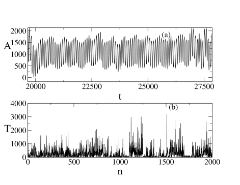
Figure 1: Panel (a): Typical time series of the heart activity of Drosophila melanogaster. The unit for time is $0.001$ s. Panel (b): Interbeat intervals for the time series of heart activity of Drosophila. As we can see the time series of the heart rate fluctuate irregularly from beat to beat.

3 Results

A part of typical time series for the heart activity of Drosophila melanogaster is presented in panel (a) of Fig. 1. From these time series we can construct time series for the interbeat intervals (presented in panel (b) of Fig. 1). Such time series are widely studied for humans [18], [19] because they can be easily measured in a noninvasive way and may have diagnostic and prognostic value. The interbeat time series of human heartbeat dynamics has (i) monofractal properties (constant $h$) for humans with heart diseases and (ii) multifractal properties (nonconstant $h$) for time series from healtly humans. As we shall see this is not the case for Drosophila.

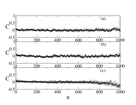
Figure 2: Autocorrelation function $C(n)$ for the time series of the heart activity of Drosophila. Panel (a) : autocorrelation for a healtly animal. Panels (b) and (c): autocorrelations for the two parents: female (panel (b)) and male (panel (c)).

The autocorrelation functions for a healtly control fly and for the parents with heart defects are shown in Fig. 2. In all three panels we observe that a significant degree of correlation exists even for large values of $n$. In addition in panel (c) we observe systematic decrease of the autocorrelation function and transition from predominantly correlated behavior for small $n$ to predominantly anticorrelated behavior for large $n$. Thus the dynamical consequences of the different genetic heart defects of Drosophila are clearly visible.

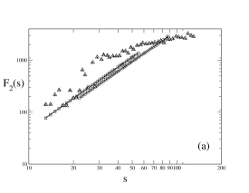
Figure 3: Panel (a): Typical forms of the fluctuation function for intermaxima time series with and without scaling properties. Fluctuation function $F_{2}(s)$ for the parents are as follows. Circles: female parent. Squares: male parent. For these time series r.m.s. fit of the power law is shown as a continuous straight line. The closeness to a straight line on the log-log scale means that the corresponding time series of the intermaxima intervals have scaling properties. For comparison typical time series for a healtly Drosophila (filled triangles) is presented. We do not observe scaling and thus we cannot calculate any fractal spectra. Panel (b): Fluctuation functions $F_{2}(s)$ and power-law r.m.s. fits (solid lines) for time series of the first generation of flies (the kids). As we see there is no drastic breaking of the scaling as it is for the healtly Drosophila of panel (a).

Panel (a) of Fig. 3 shows the fluctuation functions ( $q=2$) for a healtly Drosophila and for parent flies with heart defects. In the case of humans the normal sinus rhythm of the heartbeat activity has complex behavior similar to the behavior of a chaotic attractor [1]. The heart dynamics of humans with heart diseases may become more periodic in comparison to the heartbeat dynamics of the healtly individuals. The heartbeat dynamics of the investigated here Drosophila shows opposite behavior. We see that the fluctuation function for the healtly Drosophila does not exhibit scaling at least for small $s$ and this lack of scaling is observed for all values of the parameter $q$. The deviation from the scaling behavior for the fluctuation function means that we can not calculate any fractal spectra for the healtly Drosophila opposite to the case of the flies with genetic defects where the fluctuation function can show good scaling properties for the whole studied range of $s$. We note that the fluctuation functions for the parents seem to be very close to a straight line on a log-log scale. Thus we shall proceed with calculation of the fractal spectra. These spectra will have different properties for time series of Drosophila with different heart defects.

Figure 4: The fractal spectrum $h(q)$ for the time series of the parents. $q$ changes continuously from $-10$ to $10$. Panel (a): female parent. Panel (b): male parent

The Hurst exponent for the two parents is presented in Fig. 4. $h$ is not a constant and hence the two time series of the parents have multifractal properties. Thus multifractal cardiac dynamics can be observed not only for humans but also for much simpler animals like Drososphila.

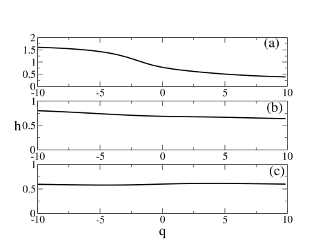
Figure 5: The fractal spectrum $h(q)$ for the time series of the first generation (the kids). From the top to the bottom the three characteristic shapes of this spectra are shown.

In figures 5 and 6 we see the kinds of spectra of the Hurst exponent characteristic for the first and second generations of flies obtained from the above-mentioned parents with genetically defect hearts. The spectra in panels (a) and (b) in Fig. 5 are of the same kinds as the spectra of the two parents. The spectrum in panel (c) has nontypical from the point of view of physics because in most physical systems $h$ decreases with increasing $q$.

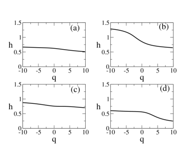
Figure 6: The fractal spectra $h(q)$ for the time series of the second generation (the kids of the kids).

For the second generation of flies we observe the two kinds of $h(q)$ spectra existing in the case of the parents plus an additional kind of spectrum with Hurst exponent which is systematically smaller than $0.5$ for positive $q$ i.e. the anticorrelations dominate the corresponding time series.

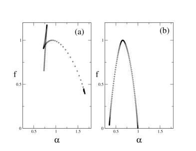
Figure 7: The fractal spectrum $f(\alpha)$ for the time series of the parents. Panel (a): female parent; Panel (b): male parent. Parameters of the spectrum in panel (b) are: $\alpha_{min}=0.35$, $\alpha_{max}=1.01$, $f_{max}=1.00$ at $\alpha=0.66$. $\alpha_{l}(0.9f_{max})=0.57$, $\alpha_{r}(0.9f_{max})=0.75$. Thus the width $\Delta(0.9f_{max})=0.18$.

The difference in the dynamical properties of the intermaxima time series for the heartbeat activity of Drosophila can be investigated by means of their $f(\alpha)$ spectra. Fig. 7 shows these spectra for the parents. For the spectra with parabolic form, the parts of elements of the time series with a given value of $\alpha$, build a partial fractal with a fractal dimension denoted by $f(\alpha)$. The top part of the spectrum which is located around some value $f(\alpha^{*})$ corresponds to the statistical most significant part of the spectrum (corresponding to the parts of the time series with the largest dimension). $f(\alpha^{*})$ gives the value of this largest dimension and we can distinguish the time series with respect to the value of $\alpha^{*}$ and the width of the spectrum around the maximum ( $\Delta=\alpha_{r}(f^{*})-\alpha_{l}(f^{*})$, where $f^{*}$ is characteristic which we shall take to be equal of $0.9f_{max}$ in order to compare the parameters of the $f(\alpha)$ spectra of all generations of Drosophila. $\alpha_{l}$ and $\alpha_{r}$ are the values of $\alpha$ corresponding to $f^{*}$ and positioned to the left and to the right with respect to the value $\alpha^{*}$ corresponding to the maximum of the $f(\alpha)$ spectrum). Wide $f(\alpha)$ spectrum corresponds to more distributed multifractal (the partial fractal dimensions are less concentrated around the maximum partial dimension $f_{max}$) and a narrow spectrum corresponds to more concentrated multifractal. Coming back to the spectra of parents in Fig. 7 we observe the typical parabolic form of the spectrum only for the male parent. Thus the form of the $f(\alpha)$ spectrum can help us to distinguish among the heart defects of Drosophila as some of these defects (and in particular the genetic defect of the female parent) can lead to nonparabolic form of the $f(\alpha)$ spectrum, i.e., to deviation from the ideal multifractal behaviour. $f_{max}=1$ for the spectrum of the male parent and its $0.9f_{max}$ width is $\Delta=0.18$. The result of the combination of the two kinds of dynamics leading to parabolic and nonparabolic $f(\alpha)$ spectra can be observed in the spectra of the two generation of flies following the parents. The characteristic spectra for the second generation are presented in Fig. 8. We observe two kinds of consequences from the form of the spectrum of the female parent (i) the nonparabolic kind of spectrum is reproduced as it can be seen in panel (b) of Fig. 8. and (ii) some (but not al) of the parameters of the parabolic spectra change. We note that for the parabolic spectra in panels (a), (c), (d) of Fig. 8 $f_{max}$ remains unchanged and equal to $1$ not only for this generation of flies but also for the parabolic spectra in the next generation shown in Fig. 9. For the second generation of flies $\alpha$ for $f_{max}$ is dispersed around $0.66$ - its value for the male parent.

Figure 8: The fractal spectra $f(\alpha)$ for the time series of the second generation (the kids). Four characteristic shapes of this spectra are shown. The parameters of the spectra of parabolic kinds are: Panel (a): $\alpha_{min}=0.24$, $\alpha_{max}=1.79$, $\alpha_{l}=0.61$, $\alpha_{r}=0.99$, $\Delta=0.28$. $f_{max}=1.00$ at $\alpha=0.80$. Panel (c): $\alpha_{min}=0.56$, $\alpha_{max}=0.72$, $\alpha_{l}=0.56$, $\alpha_{r}=0.65$, $\Delta=0.08$ $f_{max}=1.00$ at $\alpha=0.59$. Panel (d): $\alpha_{min}=0.41$, $\alpha_{max}=0.81$, $\alpha_{l}=0.54$, $\alpha_{r}=0.72$, $\Delta=0.18$. $f_{max}=1.00$ at $\alpha=0.65$.

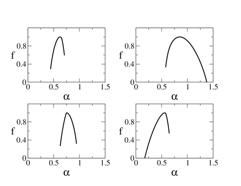
Figure 9: Parabolic fractal spectra $f(\alpha)$ for the time series of the third generation (the kids of the kids). Four characteristic shapes of this spectra are shown. Parameters of the spectra are as follows: Panel (a): $\alpha_{min}=0.44$, $\alpha_{max}=0.71$, $\alpha_{l}=0.55$, $\alpha_{r}=0.67$, $\Delta=0.12$. $f_{max}=1.00$ at $\alpha=0.65$. Panel (b): $\alpha_{min}=0.58$, $\alpha_{max}=1.40$, $\alpha_{l}=0.72$, $\alpha_{r}=1.01$, $\Delta=0.29$. $f_{max}=1.00$ at $\alpha=0.86$. Panel (c): $\alpha_{min}=0.63$, $\alpha_{max}=0.94$, $\alpha=0.72$, $\alpha_{r}=0.83$, $\Delta=0.13$.$f_{max}=1.00$ at $\alpha=0.78$. Panel (d): $\alpha_{min}=0.12$, $\alpha_{max}=0.65$, $\alpha_{l}=0.47$, $\alpha_{r}=0.60$, $\Delta=0.13$. $f_{max}=1.00$ at $\alpha=0.56$.

In the third generation of flies the nonparabolic form of the spectrum is reproduced again. From several characteristic examples of parabolic spectra of this generation which are shown in Fig.9 only one of the spectra has a wide basis. For all spectra $f_{max}=1$ and for the spectra from panels (a), (c), (d) $\Delta$ is almost the same.

4 Concluding remarks

In this paper we apply the multifractal detrended fluctuation analysis (MFDFA) to the study of Drosophila ECG time series. On the example of Drosophila we have shown that the presence of long-range correlations in the heartbeat activity is property not only of humans and complex animals and can be observed in much simpler animals as for example in Drosophila melanogaster. Opposite to the heartbeat dynamics of healtly humans which is described by broad range of Hurst exponents the intermaxima intervals of the time series of the heartbeat dynamics of healtly Drosophila do not have scaling properties and thus it cannot be described by means of scaling exponents and fractal spectra. We have shown that the presence of genetic defects can lead to long-range correlations of the heartbeat dynamics of Drosophila. The transfer of the multifractal properties from generation to generation and the similarity of the kinds and parameters of the multifractal spectra for different generations of Drosophila show that a correlation could exists between genetic properties and dynamic patterns in the heartbeat activity of simple animals like Drosophila. We can conjecture that the above correlation exists for the case of other simple animals and probably also for the case of more complex animals and ever humans.

References

- [1] Bassinngthwaighte J. B., Liebovitch L. S., West B. J. (1994). Fractal physiology. (Oxford University Press: New York).
- [2] Ivanov P. Ch. (2003). Long-range dependence in heartbeat dynamics, p.p. 339-368 in Ragarajan G. and Ding H (eds.) (2003). Processes with long-range correlations. Lecture Notes in Physics , vol. 621 (Springer: Berlin).
- [3] Skinner, J.E., Pratt, C.M., and Vybiral, T.A. (1993). A reduction in the correlation dimension of heart beat intervals proceeds imminent ventricular fibrillation in human subjects. American Heart Journal 125, 731-743.
- [4] Jonson, E., Ringo, J. and Dowse, H. (2001) Dynamin, encoded by shibire, is central to cardiac function. Journal of Experimental Zoology, 289, 81-89.
- [5] Mandelbrot B. B. (1982). The fractal geometry of the Nature. (Freeman: San Francisco).
- [6] Stanley H. E. (1999). Scaling, universality, and renormalization: Three pilars of the modern critical phenomena. Rev. Mod. Phys. 71 S358-S366.
- [7] Stanley H. E., Buldyrev S. V., Goldberger A. L., Goldberger Z. D., Havlin S., Mantegna R. N., Ossadnik S. M., Peng C.-K., Simons M. (1994). Statistical mechanics in biology: how ubiquitous are long-range correlations. Physica A 205, 214-253.
- [8] Tel T. (1988). Fractals, multifractals and thermodynamics. Zeitschrift für Naturforschung A 43, 1154-1174.
- [9] Everetsz C. J. G., Mandelbrot B. B. (1992). Multifractal measures. p.p. 921-953 in Peitgen H. -O., Jürgens, Saupe D. Chaos and fractals. New frontiers of science. Springer, New York.
- [10] Ott E. (1993). Chaos in dynamical systems. (Cambridge University Press: Cambridge).
- [11] Muzy J. F., Bacry E., Arneodo A. (1993). Multifractal formalism for fractal signals. The structure function approach versus the wavelet-transform modulus-maxima method. Physical Review E 47, 875-884.
- [12] Muzy J. F., Bacry E., Arneodo A. (1994). The multifractal formalism, revisited with wavelets. Interantional Journal of Bifurcations and Chaos. 4, 254-302.
- [13] Arneodo A., d’Aubenton-Garafa Y., Graves P. V., Muzy J. F., Thermes C. (1996) Wavelet based fractal analysis of DNA sequences. Physica D 96, 291-320.
- [14] Arneodo A., Manneville S., Muzy J. F., Roux S. G. (1999). Revealing a lognormal cascading process in turbulent velocity statistics with wavelet analysis. Philosophical Transactions of the Royal Society of London A 357, 2415-2438.
- [15] Arneodo A., Decoster N., Kestener P., Roux S. G. (2003). A Wavelet-based method for multifractal image analysis: From theoretical concepts to experimental applications. Advances in Imaging and Electron Physics 126, 1-92.
- [16] Dimitrova Z. I., Vitanov N. K. (2004). Chaotic pairwise competition. Theoretical Population Biology. 66, 1-12.
- [17] Kantelhardt J. W., Zschiegner S. A., Koscielny-Bunde E., Havlin S., Bunde A., Stanley H. E. (2002). Multifractal detrended fluctuation analysis of nonstationary time series. Physica A 316, 87-114.
- [18] Peng C. -K., Mietus J., Hausdorf J. M., Havlin S.,Stanley H. E., Goldberger A. L. (1993). Long-range anticorrelations and non-Gaussian behavior of the heartbeat. Phys. Rev. Lett. 70, 1343-1346.
- [19] Ivanov P. Ch., Amaral L. A. N., Goldberger A. L., Havlin S., Rosenblum M. G., Struzik Z. R., Stanley H. E. (1999). Multifractality in human heartbeat dynamics. Nature 399, 461-465.