Multilevel domain decomposition for electronic structure calculations

Abstract

We introduce a new multilevel domain decomposition method (MDD) for electronic structure calculations within semi-empirical and Density Functional Theory (DFT) frameworks. This method iterates between local fine solvers and global coarse solvers, in the spirit of domain decomposition methods. Using this approach, calculations have been successfully performed on several linear polymer chains containing up to 40,000 atoms and 200,000 atomic orbitals. Both the computational cost and the memory requirement scale linearly with the number of atoms. Additional speed-up can easily be obtained by parallelization. We show that this domain decomposition method outperforms the Density Matrix Minimization (DMM) method for poor initial guesses. Our method provides an efficient preconditioner for DMM and other linear scaling methods, variational in nature, such as the Orbital Minimization (OM) procedure.

1 Introduction and motivation

A central issue in computational quantum chemistry is the determination of the electronic ground state of a molecular system. For completeness and self-consistency, we now briefly introduce the problem. In particular, we present it in a mathematical way.

1.1 Standard electronic structure calculations

A molecular system is composed of $N$ electrons, modelled quantum mechanically, and a given number of nuclei, the latter being considered as classical point-like particles clamped at known positions (Born-Oppenheimer approximation). We refer to [7] for a general mathematical exposition and to [12, 19] for the chemical background. Determining the electronic ground state amounts to solving a time-independent Schrödinger equation in ${\rm IR}^{3N}$. This goal is out of reach for large values of $N$. In fact it is already infeasible for values of $N$ exceeding three or four, unless dedicated techniques are employed. Examples are stochastic-like techniques such as Diffusion Monte-Carlo approaches, or emerging techniques, such as sparse tensor products techniques [17]. Approximations of the Schrödinger equation have been developed, such as the widely used tight-binding, Hartree-Fock and Kohn-Sham models. For these three models, the numerical resolution of a problem of the following type is required: given $H$ and $S$, respectivement an $N_{b}\times N_{b}$ symmetric matrix and an $N_{b}\times N_{b}$ symmetric positive definite matrix (with $N_{b}>N$), compute a solution $D_{\star}$ of the problem

$$\left\{\begin{array}[]{l}\displaystyle Hc_{i}=\epsilon_{i}Sc_{i},\qquad\qquad\displaystyle\epsilon_{1}\leq\ldots\leq\epsilon_{N}\leq\epsilon_{N+1}\leq\ldots\leq\epsilon_{N_{b}},\\ \\ \displaystyle c_{i}^{t}Sc_{j}=\delta_{ij},\\ \\ D_{\star}=\displaystyle\sum_{i=1}^{N}c_{i}c_{i}^{t}.\end{array}\right.$$ (1.1)

Let us mention that most electronic structure calculations are performed with closed shell models [12], and that, consequently, the integer $N$ in (1.1) then is the number of electron pairs. We remark that when $S$ is the identity matrix, a solution $D_{\star}$ to (1.1) is a solution to the problem

$$\left\{\begin{array}[]{l}\hbox{\rm Find the {\em orthogonal projector} on the space spanned by the}\,N\,\hbox{\rm eigenvectors}\\ \hbox{\rm associated with the lowest}\,N\,\hbox{\rm eigenvalues of $H$.}\end{array}\right.$$ (1.2)

In (1.2), and throughout this article, the eigenvalues are counted with their multiplicities. The $N$ eigenvectors $c_{i}$, called generalized eigenvectors in order to emphasize the presence of the matrix $S$, represent the expansion in a given Galerkin basis $\left\{\chi_{i}\right\}_{1\leq i\leq N_{b}}$ of the $N$ one-electron wavefunctions. The matrix $H$ is a mean-field Hamiltonian matrix. For instance, for the Kohn-Sham model, we have

$$H_{ij}=\frac{1}{2}\int_{{\rm IR}^{3}}\nabla\chi_{i}\cdot\nabla\chi_{j}+\int_{{\rm IR}^{3}}V\chi_{i}\chi_{j}$$ (1.3)

where $V$ is a mean-field local potential. The matrix $S$ is the overlap matrix associated with the basis $\left\{\chi_{i}\right\}_{1\leq i\leq N_{b}}$:

$$S_{ij}=\displaystyle\int_{{\rm IR}^{3}}\chi_{i}\chi_{j}.$$ (1.4)

In this article, we focus on the Linear Combination of Atomic Orbitals (LCAO) approach. This is a very efficient discretization technique, using localized basis functions $\left\{\chi_{i}\right\}$, compactly supported [23] or exhibiting a gaussian fall-off [12].

It is important to emphasize what makes the electronic structure problem, discretized with the LCAO approach, specific as compared to other linear eigenvalue problems encountered in other fields of the engineering sciences (see [2, 13] for instance). First, $N_{b}$ is proportional to $N$, and not much larger than it (say $N_{b}\sim 2N$ to fix the ideas). Hence, the problem is not finding a few eigenvectors of the generalized eigenvalue problem (1.1). Second, although the matrices $H$ and $S$ are sparse for large molecular systems (see section 1.2 for details), they are not as sparse as the stiffness and mass matrices usually encountered when using finite difference or finite element methods. For example, the bandwith of $H$ and $S$ is of the order of $10^{2}$ in the numerical examples reported in section 4. Note that, in contrast, for plane wave basis set discretizations (which will not be discussed here), the parameter $N_{b}$ is much larger than $N$ (say $N_{b}\sim\,100\,N$), the matrix $S$ is the identity matrix and the matrix $H$ est full. Third, and this is a crucial point, the output of the calculation is the matrix $D_{\star}$ and not the generalized eigenvectors $c_{i}$ themselves. This is the fundamental remark allowing the construction of linear scaling methods (see section 1.2).

A solution $D_{\star}$ of (1.1) is

$$D_{\star}=C_{\star}C_{\star}^{t}$$ (1.5)

where $C_{\star}$ is a solution to the minimization problem

$$\inf\biggl{\{}\mbox{{Tr}}\Big{(}HCC^{t}\Big{)},\quad C\in{\mathcal{M}}^{N_{b},N}({\rm IR}),\;C^{t}SC=I_{N}\biggr{\}}.$$ (1.6)

Note that the energy functional $\mbox{{Tr}}\Big{(}HCC^{t}\Big{)}$ can be given the more symmetric form $\mbox{{Tr}}\Big{(}C^{t}HC\Big{)}$. Here and below, ${\mathcal{M}}^{k,l}$ denotes the vector space of the $k\times l$ real matrices. Notice that (1.6) has many minimizers: if $C_{\star}$ is a minimizer, so is $C_{\star}U$ for any orthogonal $N\times N$ matrix $U$. However, under the standard assumption that the $N$-th eigenvalue of $H$ is strictly lower than the $(N+1)$-th one, the matrix $D^{\ast}$ defined by (1.5) does not in fact depend on the choice of the minimizer $C_{\star}$ of (1.6). Notice also that (1.1) are not the Euler-Lagrange equations of (1.6) but that any critical point of (1.6) is obtained from a solution of (1.1) by an orthogonal transformation of the columns of $C_{\star}=\displaystyle\left(c_{1}|\cdots|c_{N}\right)$.

The standard approach to compute $D_{\star}$ is to solve the generalized eigenvalue problem (1.1) and then construct $C_{\star}$ thus $D_{\star}$ by collecting the lowest $N$ generalized eigenvectors of $H$. This approach is employed when the number $N$ of electrons (or electron pairs) is not too large, say smaller than $10^{3}$.

1.2 Linear scaling methods

One of the current challenges of Computational Chemistry is to lower the computational complexity $N^{3}$ of this solution procedure. A linear complexity $N$ is the holy grail. There are various existing methods designed for this purpose. Surveys on such methods are [6, 11]. Our purpose here is to introduce a new method, based on the domain decomposition paradigm. We remark that the method introduced here is not the first occurrence of a method based on a decomposition of the matrix $H$ [24], but a significant methodological improvement is fulfilled with the present method. To the best of our knowledge, such methods only consist of local solvers complemented by a crude global step. The method introduced below seems to be the first one really exhibiting the local/global paradigm in the spirit of methods used in other fields of the engineering sciences. Numerical obervations confirm the major practical interest methodological improvement.

Why is a linear scaling plausible for computing $D_{\star}$? To justify the fact that the cubic scaling is an estimate by excess of the computational task required to solve (1.1), we argue that the matrix does not need to be diagonalized. As mentioned above, only the orthogonal projector on the subspace generated by the lowest $N$ eigenvectors is to be determined and not the explicit values of these lowest $N$ eigenvectors. But in order to reach a linear complexity, appropriate assumptions are necessary, both on the form of the matrices $H$ and $S$, and on the matrix $D_{\star}$ solution to (1.1):

• (H1). The matrices $H$ and $S$ are assumed sparse, in the sense that, for large systems, the number of non-zero coefficients scales as $N$. This assumption is not restrictive. In particular, it follows from (1.3) and (1.4) that it is automatically satisfied for Kohn-Sham models as soon as the basis functions are localized in real space, which is in particular the case for the widely used atomic orbital basis sets [7];

• (H2). A second assumption is that the matrix $D_{\star}$ built from the solution to (1.1) is also sparse. This condition seems to be fulfilled as soon as the relative gap

  $$\gamma=\frac{\epsilon_{N+1}-\epsilon_{N}}{\epsilon_{N_{b}}-\epsilon_{1}}.$$ (1.7)

  deduced from the solution of (1.1) is large enough. As explained in section 2 below, this observation can be supported by qualitative physical arguments. On the other hand, we are not aware of any mathematical argument of linear algebra that would justify assumption (H2) in a general setting.

We assume (H1)-(H2) in the following. Current efforts aim at treating cases when the second assumption is not fulfilled, which in particular corresponds to the case of conducting materials. The problem (1.2) is then extremely difficult because the gap $\gamma$ in (1.7) being very small, the matrix $D$ is likely to be dense. Reaching linear complexity is then a challenging issue, unsatisfactorily solved to date. State of the art linear scaling methods presented in the literature experience tremendous difficulties (to say the least) in such cases. It is therefore reasonable to improve in a first step the existing methods in the setting of assumption (H2), before turning to more challenging issues.

Before we get to the heart of the matter, we would like to point out the following feature of the problem under consideration.

In practice, Problem (1.1) has to be solved repeatedly. For instance, it is the inner loop in a nonlinear minimization problem where $H$ depends self-consistently on $D_{\star}$. We refer to [8, 14] for efficient algorithms to iterate on this nonlinearity and to [7] for a review on the subject. Alternatively, or in addition to the above, problem (1.1) is parametrized by the positions of the nuclei (both the mean-field operator $H$ and the overlap matrix $S$ indeed depend on these positions), and these positions may vary. This is the case in molecular mechanics (find the optimal configuration of nuclei that gives the lowest possible energy to the molecular system), and in molecular dynamics as well (the positions of nuclei follow the Newton law of motion in the mean-field created by the electrons). In either case, problem (1.1) is not be solved from scratch. Because of previous calculations, we may consider we have at our disposal a good initial guess for the solution. The latter comes from e.g. previous positions of nuclei, or previous iterations in the outer loop of determination of $H$. In difficult cases it may even come from a previous computation with a coarse grained model. In other words, the question addressed reads solving Problem (1.1) for some $H+\delta H$ and $S+\delta S$ that are small perturbations of previous $H$ and $S$ for which the solution is known. This specific context allows for a speed up of the algorithm when the initial guess is sufficiently good. This is the reason why, in the following, we shall frequently make distinctions between bad and good initial guesses.

2 Localization in Quantum Chemistry

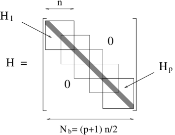
The physical system we consider is a long linear molecule (for instance a one-dimensional polymer or a nanotube). Let us emphasize that we do not claim a particular physical relevance of this system. This is for the purpose of illustration. We believe the system considered to be a good representative of a broad class of large molecular systems that may be encountered practically. Each atomic orbital $\chi_{i}$ is centered on one nucleus. Either it is supported in a ball of small radius [20] (in comparison to the size of the macromolecule under study), or it has a rapid exponential-like or Gaussian-like [10] fall-off. The atomic orbitals are numbered following the orientation of the molecule. Then, the mean-field Hamiltonian matrix $H$ whose entries are defined by (1.3) has the band structure shown in Figure 1.

Although the eigenvectors of $H$ are a priori delocalized (most of their coefficients do not vanish), it seems to be possible to build a $S$-orthonormal basis of the subspace generated by the lowest $N$ eigenvectors of $H$, consisting of localized vectors (only a few consecutive coefficients are non zero). This is motivated by a physical argument of locality of the interactions [16]. For periodic systems, the localized vectors correspond to the so-called Wannier orbitals [4]. It can be proven that in this case, the larger the band gap, the better the localization of the Wannier orbitals [15]. For insulators, the Wannier orbitals indeed enjoy an exponential fall-off rate proportional to the band gap. For conductors, the fall-off is only algebraic. As mentioned in the introduction, we only consider here the former case. This allows us to assume that there exists some integer $q\ll N_{b}$, such that $N_{b}/q$ is an integer, for which all of these localized functions can be essentially expanded on $q$ consecutive atomic orbitals. Denoting by $n=2q$, we can therefore assume a good approximation of a solution $C_{\star}$ to (1.6) exists, with the block structure displayed on Figure 2. Note that each block $C_{i}$ only overlaps with its nearest neighbors. Correspondingly, we introduce the block structure of $H$ displayed on Figure 3. The matrix $D$ constructed from a block matrix $C$ using (1.5) has the structure represented in Figure 4 and satisfies the constraints $D=D^{t}$, $D^{2}=D$, Tr($D)$ = $N$.

Let us point out that the integers $q$ and $n=2q$ depend on the band gap, not on the size of the molecule. The condition $n=2q$ is only valid for $S=I_{N_{b}}$. For $S\not=I_{N_{b}}$, it is replaced by $n=2q+nbs$ where $2\,nbs-1$ is the bandwidth of the matrix $S$.

The domain decomposition algorithm we propose aims at searching an approximate solution to (1.6) that has the block structure described above.

For simplicity, we now present our method assuming that $S=I_{N_{b}}$, i.e. that the Galerkin basis $\left\{\chi_{i}\right\}_{1\leq i\leq N_{b}}$ is orthonormal. The extension of the method to the case when $S\neq I_{N_{b}}$ is straightforward. Problem (1.6) then reads

$$\inf\biggl{\{}\mbox{{Tr}}\Big{(}HCC^{t}\Big{)},\quad C\in{\mathcal{M}}^{N_{b},N}({\rm IR}),\;C^{t}C=I_{N}\biggr{\}}.$$ (2.1)

Our approach consists in solving an approximation of problem (2.1) obtained by minimizing the exact energy $\displaystyle\mbox{{Tr}}\Big{(}HCC^{t}\Big{)}$ on the set of the matrices $C$ which have the block structure displayed on Figure 2 and satisfy the constraint $C^{t}C=I_{N}$. The resulting minimization problem can be recast as

$$\mbox{{inf}}\bigg{\{}\sum_{i=1}^{p}\mbox{{Tr}}\left(H_{i}C_{i}C_{i}^{t}\right), C_{i}\in{\mathcal{M}}^{n,m_{i}}({\rm IR}),\quad m_{i}\in{\rm IN},\quad C_{i}^{t}C_{i}=I_{m_{i}}\quad\forall\;1\leq i\leq p,$$ (2.2)

$$C_{i}^{t}TC_{i+1}=0\quad\forall\;1\leq i\leq p-1,\quad\sum_{i=1}^{p}m_{i}=N\bigg{\}}.$$

In the above formula, $T\in{\cal M}^{n,n}({\rm IR})$ is the matrix defined by

$$T_{kl}=\left\{\begin{array}[]{ll}1&\mbox{ if }k-l=q\\ 0&\mbox{ otherwise}\end{array}\right.$$ (2.3)

and $H_{i}\in{\cal M}^{n,n}({\rm IR})$ is a symmetric submatrix of $H$ (see Figure 3). Indeed,

and

In this way, we replace the $\frac{N(N+1)}{2}$ global scalar constraints $C^{t}C=I_{N}$ involving vectors of size $N_{b}$, by the $\sum_{i=1}^{p}\frac{m_{i}(m_{i}+1)}{2}$ local scalar constraints $C_{i}^{t}C_{i}=I_{m_{i}}$ and the $\sum_{i=1}^{p-1}m_{i}m_{i+1}$ local scalar constraints $C_{i}^{t}TC_{i+1}=0$, involving vectors of size $n$. We would like to emphasize that we can obtain in this way a basis of the vector space generated by the lowest $N$ eigenvectors of $H$, but not the eigenvectors themselves. This method is therefore not directly applicable to standard diagonalization problems.

Our algorithm searches for the solution to (2.2), not to (2.1). More rigorously stated, we search for the solution to the Euler-Lagrange equations of (2.2):

$$\left\{\begin{array}[]{ccll}\displaystyle H_{i}C_{i}&=&C_{i}E_{i}+T^{t}C_{i-1}\Lambda_{i-1,i}+TC_{i+1}\Lambda_{i,i+1}^{t}&\qquad 1\leq i\leq p,\\ \displaystyle C_{i}^{t}C_{i}&=&I_{m_{i}}&\qquad 1\leq i\leq p,\\ \displaystyle C_{i}^{t}TC_{i+1}&=&0&\qquad 1\leq i\leq p-1,\end{array}\right.$$ (2.4)

where by convention

$$C_{0}=C_{p+1}=0.$$ (2.5)

The matrices $(E_{i})_{1\leq i\leq p}$ and $(\Lambda_{i,i+1})_{1\leq i\leq p-1}$ respectively denote the matrices of Lagrange multipliers associated with the orthonormality constraints $C_{i}^{t}C_{i}=I_{m_{i}}$ and $C_{i}^{t}TC_{i+1}=0$. The $m_{i}\times m_{i}$ matrix $E_{i}$ is symmetric. The matrix $\Lambda_{i,i+1}$ is of size $m_{i}\times m_{i+1}$. The above equations can be easily derived by considering the Lagrangian

$${\cal L}\left(\left\{C_{i}\right\},\left\{E_{i}\right\},\left\{\Lambda_{i,i+1}\right\}\right) = \sum_{i=1}^{p}{\rm Tr}\left(H_{i}C_{i}C_{i}^{t}\right)+\sum_{i=1}^{p}{\rm Tr}\left(\left(C_{i}^{t}C_{i}-I_{m_{i}}\right)E_{i}\right)$$

$$+\sum_{i=1}^{p-1}{\rm Tr}\left(C_{i}^{t}TC_{i+1}\Lambda_{i,i+1}^{t}\right).$$

The block structure imposed on the matrices clearly lowers the dimension of the search space we have to explore. However, this simplification comes at a price. First, problem (2.2) only approximates problem (2.1). Second, (2.2) may have local, non global, minimizers, whereas all the local minimizers of (2.1) are global. There are thus a priori many spurious solutions of the Euler Lagrange equations (2.4) associated with (2.2).

A point is that the sizes $(m_{i})_{1\leq i\leq p}$ are not a priori prescribed. In our approach, they are ajusted during the iterations. We shall see how in the sequel.

3 Description of the domain decomposition algorithm

3.1 Description of a simplified form

For pedagogic purpose, we first consider the following problem

$$\inf\left\{\langle H_{1}Z_{1},Z_{1}\rangle+\langle H_{2}Z_{2},Z_{2}\rangle,\quad Z_{i}\in{{\rm IR}}^{N_{b}},\;\langle Z_{i},Z_{i}\rangle=1,\;\langle Z_{1},Z_{2}\rangle=0\right\}.$$ (3.1)

Problem (3.1) is a particular occurence of (2.2). We have denoted by $\langle\cdot,\cdot\rangle$ the standard Euclidean scalar product on ${{\rm IR}}^{N_{b}}$.

For (3.1), the algorithm is defined in the following simplified form. Choose $(Z_{1}^{0},Z_{2}^{0})$ satisfying the constraints and construct the sequence $(Z_{1}^{k},Z_{2}^{k})_{k\in{\rm IN}}$ by the following iteration procedure. Assume $(Z_{1}^{k},Z_{2}^{k})$ is known, then

• Local step. Solve

  $$\left\{\begin{array}[]{lll}\widetilde{Z}_{1}^{k}=\mbox{{arginf}}\big{\{}\langle H_{1}Z_{1},Z_{1}\rangle,\,\,Z_{1}\in{{\rm IR}}^{N_{b}},\,\,\,\langle Z_{1},Z_{1}\rangle=1\,\,\langle Z_{1},Z_{2}^{k}\rangle=0\big{\}},\\ \widetilde{Z}_{2}^{k}=\mbox{{arginf}}\big{\{}\langle H_{2}Z_{2},Z_{2}\rangle,\,\,Z_{2}\in{{\rm IR}}^{N_{b}},\,\,\,\langle Z_{2},Z_{2}\rangle=1\,\,\langle\widetilde{Z}_{1}^{k},Z_{2}\rangle=0\big{\}}\;;\end{array}\right.$$ (3.2)

• Global step. Solve

  $$\alpha^{\ast}=\mbox{{arginf}}\big{\{}\langle H_{1}Z_{1},Z_{1}\rangle+\langle H_{2}Z_{2},Z_{2}\rangle,\;\alpha\in{{\rm IR}}\big{\}}$$ (3.3)

  where

  $$Z_{1}=\frac{\widetilde{Z}_{1}^{k}+\alpha\widetilde{Z}_{2}^{k}}{\sqrt{1+\alpha^{2}}},\,\,Z_{2}=\frac{-\alpha\widetilde{Z}_{1}^{k}+\widetilde{Z}_{2}^{k}}{\sqrt{1+\alpha^{2}}},$$ (3.4)

  and set

  $$Z_{1}^{k+1}=\frac{\widetilde{Z}_{1}^{k}+\alpha^{\ast}\widetilde{Z}_{2}^{k}}{\sqrt{1+(\alpha^{\ast})^{2}}},\quad Z_{2}^{k+1}=\frac{-\alpha^{\ast}\widetilde{Z}_{1}^{k}+\widetilde{Z}_{2}^{k}}{\sqrt{1+(\alpha^{\ast})^{2}}}.$$ (3.5)

In the $k$-th iteration of the local step, we first fix $Z_{2}=Z_{2}^{k}$ and optimize over $Z_{1}$ to obtain $\tilde{Z}_{1}^{k}$. Then we fix $Z_{1}=\tilde{Z}_{1}^{k}$ and optimize over $Z_{2}$ to obtain $\tilde{Z}_{2}^{k}$. This local step monotonically reduces the objective function, however, it may not converge to the global optimum. The technical problem is that the Lagrange multipliers associated with the constraint $\langle Z_{1},Z_{2}\rangle=0$ may converge to different values in the two subproblems associated with the local step. In the global step, we optimize the sum $\langle H_{1}Z_{1},Z_{1}\rangle+\langle H_{2}Z_{2},Z_{2}\rangle$ over the subspace spanned by $\tilde{Z}_{1}^{k}$ and $\tilde{Z}_{2}^{k}$, subject to the constraints in (3.1). The global step again reduces the value of the objective function since $\tilde{Z}_{1}^{k}$ and $\tilde{Z}_{2}^{k}$ are feasible in the global step. It can be shown that the combined algorithm (local step + global step) monotonically decreases the objective function and globally converges to an optimal solution of (3.1).

This algorithm operates at two levels: a fine level where we solve two problems of dimension $N_{b}$ rather than one problem of dimension $2N_{b}$; a coarse level where we solve a problem of dimension $2$. Left by itself, the fine step converges to a suboptimal solution of (3.1). Combining the fine step with the global step yields convergence to a global optimum.

In addition to providing a pedagogic view on the general algorithm presented in the following section, the simplified form (3.2)-(3.5) has a theoretical interest. In contrast to the general algorithm for which we cannot provide a convergence analysis, the simplified form (3.2)-(3.5) may be analyzed mathematically, at least in the particular situation when $H_{1}=H_{2}=H$. Then solving (3.1) amounts to searching for the lowest two eigenelements of the matrix $H$. Notice that the global step (3.3)-(3.5) is then unnecessary because the functional to minimize in (3.3) does not depend on $\alpha$.

However, we can show that the iterations (3.2) converge in the following sense. The 2-dimensional vector space spanned by the lowest two eigenvalues of $H$ is reached asymptotically. This occurs under an appropriate condition on the matrix $H$. The latter is a condition of separation of the eigenvalues, namely $\displaystyle\epsilon_{2}-\epsilon_{1}<\epsilon_{3}-\epsilon_{2}$ with obvious notation. The gap $\epsilon_{3}-\epsilon_{2}$ gives the speed of convergence. For brevity, we do not detail the proof here (see [5]). Future work on the numerical analysis of more general cases is in progress.

3.2 Description of the algorithm

We define, for all $p$-tuple $(C_{i})_{1\leq i\leq p}$,

$${\mathcal{E}}\Big{(}(C_{i})_{1\leq i\leq p}\Big{)}=\sum_{i=1}^{p}\mbox{{Tr}}\Big{(}H_{i}C_{i}C_{i}^{t}\Big{)},$$ (3.6)

and set by convention

$$U_{0}=U_{p}=0.$$ (3.7)

We introduce an integer $\epsilon$, initialized to one, that will alternate between the values zero and one during the iterations.

At iteration $k$, we have at hand a set of block sizes $(m_{i}^{k})_{1\leq i\leq p}$ and a set of matrices $(C_{i}^{k})_{1\leq i\leq p}$ such that $C_{i}^{k}\in{\cal M}^{n,m_{i}^{k}}({\rm IR})$, $[C_{i}^{k}]^{t}C_{i}^{k}=I_{m_{i}^{k}}$, $[C_{i}^{k}]^{t}TC_{i+1}^{k}=0$. We now explain how to compute the new iterate $(m_{i}^{k+1})_{1\leq i\leq p}$, $(C_{i}^{k+1})_{1\leq i\leq p}$.

Multilevel Domain Decomposition (MDD) algorithm

1. $\bullet$ Step 1: Local fine solver.

   1. For each $i$, diagonalize the matrix $H_{2i+\epsilon}$ in the subspace

      $$V_{2i+\epsilon}^{k}=\left\{x\in{\rm IR}^{n},\quad\left[C_{2i+\epsilon-1}^{k}\right]^{t}Tx=0,\quad x^{t}TC_{2i+\epsilon+1}^{k}=0\right\},$$

      i.e. diagonalize $P_{2i+\epsilon}^{k}H_{2i+\epsilon}P_{2i+\epsilon}^{k}$ where $P_{2i+\epsilon}^{k}$ is the orthogonal projector on $V_{2i+\epsilon}^{k}$. This provides (at least) $n-m_{2i+\epsilon-1}^{k}-m_{2i+\epsilon+1}^{k}$ real eigenvalues $\lambda_{2i+\epsilon,1}^{k}\leq\lambda_{2i+\epsilon,2}^{k}\leq\cdots$ and associated orthonormal vectors $x_{2i+\epsilon,j}^{k}$. The latter are $T$-orthogonal to the column vectors of $C_{i-1}^{k}$ and $C_{i+1}^{k}$.

   2. Sort the eigenvalues $(\lambda_{2i+\epsilon,j}^{k})_{i,j}$ in increasing order, and select the lowest $\displaystyle\sum_{i}m_{2i+\epsilon}$ of them. For each $i$, collect in block $\#2i+\epsilon$ the eigenvalues $\lambda^{k}_{2i+\epsilon,j}$ selected. New intermediate block sizes $\bar{m}_{2i+\epsilon}^{k}$ are defined.

   3. For each $i$, collect the lowest $\bar{m}_{2i+\epsilon}^{k}$ vectors $x_{2i+\epsilon,j}^{k}$ in the $n\times\bar{m}_{2i+\epsilon}^{k}$ matrix $\overline{C}_{2i+\epsilon}^{k}$.

   4. For each $i$, diagonalize the matrix $H_{2i+\epsilon+1}$ in the subspace

      $$V_{2i+\epsilon+1}^{k}=\left\{x\in{\rm IR}^{n},\quad\left[\overline{C}_{2i+\epsilon}^{k}\right]^{t}Tx=0,\quad x^{t}T\overline{C}_{2i+\epsilon+2}^{k}=0\right\}$$

      in order to get eigenvalues $\lambda_{2i+\epsilon+1,1}^{k}\leq\lambda_{2i+\epsilon+1,2}^{k}\leq\cdots$ and associated orthonormal vectors $x_{2i+\epsilon+1,j}^{k}$. The latter are $T$-orthogonal to the column vectors of $\overline{C}_{2i+\epsilon}^{k}$ and $\overline{C}_{2i+\epsilon+2}^{k}$.

   5. Sort all the eigenvalues $\displaystyle\bigl{\{}(\lambda_{2i+\epsilon+1,j}^{k})_{i,j},(\lambda_{2i+\epsilon,j}^{k})_{i,j}\bigr{\}}$ in increasing order. Select the lowest $N$. For each $l$, collect in block $\#l$ the eigenvalues $\lambda^{k}_{l,j}$ selected. New intermediate block sizes $(m_{l}^{k+1})_{1\leq l\leq p}$ are thus defined.

   6. Set $\widetilde{C}_{l}^{k}=\displaystyle\left[x_{l,1}^{k}|\cdots|x_{l,m_{l}^{k+1}}^{k}\right]$.

   7. Replace $\epsilon$ by $1-\epsilon$ and proceed to step 2 below.

2. $\bullet$ Step 2: global coarse solver. Solve

   $${\mathcal{U}}^{\ast}=\mbox{{arginf}}\Big{\{}f({\mathcal{U}}),\;{\mathcal{U}}=(U_{i})_{i},\;\forall 1\leq i\leq p-1\;\;U_{i}\in{\mathcal{M}}^{m_{i+1},m_{i}}({\rm IR})\Big{\}},$$ (3.8)

   where

   $$f({\mathcal{U}})={\mathcal{E}}\bigg{(}\Big{(}C_{i}({\mathcal{U}})\big{(}C_{i}({\mathcal{U}})^{t}C_{i}({\mathcal{U}})\big{)}^{-\frac{1}{2}}\Big{)}_{i}\bigg{)},$$ (3.9)

   and

   $$C_{i}({\mathcal{U}})=\widetilde{C}_{i}^{k}+T\widetilde{C}_{i+1}^{k}U_{i}\Big{(}[\widetilde{C}_{i}^{k}]^{t}TT^{t}\widetilde{C}_{i}^{k}\Big{)}-T^{t}\widetilde{C}_{i-1}^{k}U_{i-1}^{t}\Big{(}[\widetilde{C}_{i}^{k}]^{t}T^{t}T\widetilde{C}_{i}^{k}\Big{)}.$$ (3.10)

   Next set, for all $1\leq i\leq p$,

   $$C_{i}^{k+1}=C_{i}\big{(}{\mathcal{U}}^{\ast}\big{)}\;\left(C_{i}\big{(}{\mathcal{U}}^{\ast}\big{)}^{t}\,C_{i}\big{(}{\mathcal{U}}^{\ast}\big{)}\right)^{-1/2}\;.$$ (3.11)

   Note that $\displaystyle\left[C_{i}^{k+1}\right]^{t}TC_{i+1}^{k+1}=0$ (this follows from $T^{2}=0$).

We think of the even indexed unknowns $C_{2i}$ as the black variables and the odd indexed unknowns $C_{2i+1}$ as the white variables. In the first phase of the local fine solver, we optimize over the white variables while holding the black variables fixed. In the second phase of the local fine solver, we optimize over the black variables while holding the white variables fixed. In the global step, we perturb each variable by a linear combination of the adjacent variables. The matrices ${{\mathcal{U}}}=(U_{i})_{i}$ in (3.8) play the same role as the real parameter $\alpha$ in (3.3). The perturbation is designed so that the constraints are satisfied. The optimization is performed over the matrices generating the linear combinations. In the next iteration, we interchange the order of the optimizations: first optimize over the black variables while holding the white variables fixed, then optimize over the white variables while holding the black variables fixed.

Let us point out that an accurate solution to (3.8) is not needed. In practice, we reduce the computational cost of the global step, by using again a domain decomposition method. The blocks $(C_{i})_{1\leq i\leq p}$ are collected in $r$ overlapping groups $(G_{l})_{1\leq l\leq r}$ as shown in Figure 5. Problem (3.8) is solved first for the blocks $(G_{2l+1})$, next for the blocks $(G_{2l})$. Possibly, this procedure is repeated a few times. The advantage of this strategy is that the computational time of the global step scales linearly with $N$. In addition, it is parallel in nature. The solution of (3.8) for a given group is performed by a few steps of a Newton-type algorithm. Other preconditioned iterative methods could also be considered.

3.3 Comments on the local step

The local step is based on a checkerboard iteration technique.

When $\epsilon=1$, steps 1a-1c search for a solution $(\bar{m}_{2i+1}^{k},\overline{C}_{2i+1}^{k})_{i}$ to the problem

$$\mbox{{inf}}\bigg{\{}\sum_{i}\mbox{{Tr}}\left(H_{2i+1}C_{2i+1}C_{2i+1}^{t}\right), C_{2i+1}\in{\mathcal{M}}^{n,m_{2i+1}}({\rm IR}),\quad C_{2i+1}^{t}C_{2i+1}=I_{m_{2i+1}},$$

$$[C_{2i}^{k}]^{t}TC_{2i+1}=0,\quad C_{2i+1}^{t}TC_{2i+2}^{k}=0,$$

$$m_{2i+1}\in{\rm IN},\quad\sum_{i}m_{2i+1}=\sum_{i}m_{2i+1}^{k}\bigg{\}}.$$

During steps 1a-1c, the “white” blocks $C_{2i}^{k}$ are kept fixed. The “black” blocks $C_{2i+1}^{k}$ are optimized under the orthogonality constraints imposed by the “white” blocks. A point is that most of the computational effort can be done in parallel. Indeed, for $p$ even, say, performing step 1a amounts to solving $p/2$ independent diagonalisation problems of size $n$.

Likewise, steps 1d-1f solve

$$\mbox{{inf}}\bigg{\{}\sum_{i=1}^{p}\mbox{{Tr}}\left(H_{i}C_{i}C_{i}^{t}\right), C_{i}\in{\mathcal{M}}^{n,m_{i}}({\rm IR}),\quad C_{i}^{t}C_{i}=I_{m_{i}},\quad m_{i}\in{\rm IN},\quad\sum_{i}m_{i}=N$$

$$[\overline{C}_{2j-1}^{k}]^{t}TC_{2j}=0,\quad[C_{2j}]^{t}T[\overline{C}_{2j+1}]^{k}=0,$$

$$0\leq m_{2j+1}\leq\bar{m}_{2j+1}^{k},\quad C_{2j+1}\subset\overline{C}_{2j+1}^{k}\bigg{\}},$$

where the notation $C_{2j+1}\subset\overline{C}_{2j+1}^{k}$ means that each column of $C_{2j+1}$ is a column of $\overline{C}_{2j+1}^{k}$. Here again, most of the computational effort can be performed in parallel.

When $\epsilon=1$, “black” vectors (i.e. vectors belonging to blocks with odd indices) are allowed to become “white” vectors, but the reverse is forbidden. In order to symmetrize the process, $\epsilon$ is replaced by $1-\epsilon$ in the next iteration.

We wish to emphasize that, although called local, this step already accounts for some global concern. Indeed, and it is a key point of the local step, substeps (b) and (e) sort the complete set of eigenvalues generated locally. This, together with the update of the size $m_{i}$ of the blocks, allows for a preliminary propagation of the information throughout the whole system. The global step will complement this.

Finally, let us mention that in the local steps, (approximate) $T$-orthogonality is obtained by a Householder orthonormalization process. The required orthonormality criterion is

$$\forall\;1\leq i\leq p-1,\quad\big{\|}[\tilde{C}^{k}_{i}]^{t}T\tilde{C}^{k}_{i+1}\big{\|}\leq\epsilon_{L},$$ (3.12)

where $\epsilon_{L}>0$ is a threshold to be chosen by the user.

3.4 Comments on the global step

Let us briefly illustrate the role played by the global step. For simplicity, we consider the case of two blocks of same initial size $m_{1}=m_{2}=m$ and we assume that $m_{1}$ and $m_{2}$ do not vary during the iterations. If only the local step is performed, then the new iterate

$$(C^{k+1}_{1},C_{2}^{k+1})=(\widetilde{C}_{1}^{k},\widetilde{C}_{2}^{k})$$

does not necessarily satisfies (2.4). Indeed, there is no reason why the Lagrange multipliers corresponding to the two contraints $C^{t}TC_{2}^{k}=0$ (step 1a when $\epsilon=1$) on the one hand and $[\widetilde{C}_{1}^{k}]^{t}TC=0$ (step 1d when $\epsilon=1$) on the other hand should be the same. The global step asymptotically enforces the equality of Lagrange multipliers. This is a way to account for a global feature of the problem.

Let us emphasize this specific point. Assume $U^{\ast}=0$ in the global step of the $k$-th iteration of the algorithm, or in other words that the global step is not effective at the $k$-th iteration. Then it implies that the output $(\widetilde{C}_{1},\widetilde{C}_{2})=(\widetilde{C}_{1}^{k},\widetilde{C}_{2}^{k})$ of the local step already satisfies (2.4). Indeed,

$$f(U)=\mbox{{Tr}}\Big{(}J_{1}(U)C_{1}(U)^{t}H_{1}C_{1}(U)\Big{)}+\mbox{{Tr}}\Big{(}J_{2}(U)C_{2}(U)^{t}H_{2}C_{2}(U)\Big{)}$$ (3.13)

with $J_{i}(U)=\Big{(}C_{i}(U)^{t}C_{i}(U)\Big{)}^{-1}$ for $i=1,2$. Since

$$\Big{(}J_{1}(U)\Big{)}^{-1} = I_{m}+\Big{(}\widetilde{C}_{1}^{t}TT^{t}\widetilde{C}_{1}\Big{)}U^{t}\Big{(}\widetilde{C}_{2}^{t}T^{t}T\widetilde{C}_{2}\Big{)}U\Big{(}\widetilde{C}_{1}^{t}TT^{t}\widetilde{C}_{1}\Big{)},$$

$$\Big{(}J_{2}(U)\Big{)}^{-1} = I_{m}+\Big{(}\widetilde{C}_{2}^{t}T^{t}T\widetilde{C}_{2}\Big{)}U\Big{(}\widetilde{C}_{1}^{t}TT^{t}\widetilde{C}_{1}\Big{)}U^{t}\Big{(}\widetilde{C}_{2}^{t}T^{t}T\widetilde{C}_{2}\Big{)},$$

we have $\nabla J_{1}(0)=\nabla J_{2}(0)=0$. The matrix $U$ being a square matrix of dimension $m$, for all $1\leq i,j\leq m$,

$$\displaystyle\frac{1}{2}\frac{\partial f}{\partial U_{ij}}(0) = \displaystyle\mbox{{Tr}}\bigg{(}\left[\frac{\partial C_{1}}{\partial U_{ij}}(0)\right]^{t}H_{1}\widetilde{C}_{1}\bigg{)}+\mbox{{Tr}}\bigg{(}\left[\frac{\partial C_{2}}{\partial U_{ij}}(0)\right]^{t}H_{2}\widetilde{C}_{2}\bigg{)}$$ (3.14)

$$= \displaystyle\bigg{(}\Big{(}\widetilde{C}_{1}^{t}TT^{t}\widetilde{C}_{1}\Big{)}\widetilde{C}_{1}^{t}H_{1}T\widetilde{C}_{2}\bigg{)}_{ji}-\bigg{(}\widetilde{C}_{1}^{t}TH_{2}\widetilde{C}_{2}\Big{(}\widetilde{C}_{2}^{t}T^{t}T\widetilde{C}_{2}\Big{)}\bigg{)}_{ji}$$

$$= \displaystyle\bigg{(}\Big{(}\widetilde{C}_{1}^{t}TT^{t}\widetilde{C}_{1}\Big{)}(\Lambda_{1}-\Lambda_{2})\Big{(}\widetilde{C}_{2}^{t}T^{t}T\widetilde{C}_{2}\Big{)}\bigg{)}_{ji},$$

where $\Lambda_{1}$ and $\Lambda_{2}$ are defined by

$$\left\{\begin{array}[]{ccc}\displaystyle H_{1}\widetilde{C}_{1}=\widetilde{C}_{1}E_{1}+T\widetilde{C}_{2}\Lambda_{1}^{t},\\ \displaystyle H_{2}\widetilde{C}_{2}=\widetilde{C}_{2}E_{2}+T^{t}\widetilde{C}_{1}\Lambda_{2}.\\ \end{array}\right.$$ (3.15)

As $U^{\ast}=0$ implies

$$\forall\;1\leq i,j\leq m\quad\frac{\partial f}{\partial U_{ij}}(0)=0,$$ (3.16)

we conclude that $\Lambda_{1}=\Lambda_{2}$ if the matrices $\Big{(}\widetilde{C}_{1}^{t}TT^{t}\widetilde{C}_{1}\Big{)}$ and $\Big{(}\widetilde{C}_{2}^{t}T^{t}T\widetilde{C}_{2}\Big{)}$ are invertible, which is generally the case when $n\gg 2m$. Consequently, (2.4) is satisfied by $(\widetilde{C}_{1},\widetilde{C}_{2})$.

On the other hand, when $n$ is not much larger that $2m$, the above matrices are not invertible and (2.4) is usually not satisfied. In this case, the global step is slightly modified in order to recover (2.4) and thus improve the efficiency of the global step. We replace (3.10) by

$$\forall\;1\leq i\leq p,\quad C_{i}({\mathcal{U}})=\tilde{C}_{i}^{k}+T\widehat{C}_{i+1}^{k}U_{i}\Big{(}[\widehat{C}_{i}^{k}]^{t}TT^{t}\widehat{C}_{i}^{k}\Big{)}-T^{t}\widehat{C}_{i-1}^{k}U_{i-1}^{t}\Big{(}[\widehat{C}_{i}^{k}]^{t}T^{t}T\widehat{C}_{i}^{k}\Big{)}$$ (3.17)

where $\widehat{C}_{i}^{k}$ is a block formed by vectors collected in the vector space defined by $\widetilde{C}_{i}^{k}$. These vectors are selected using a modified Gram-Schmidt orthonormalization process. The size of the blocks $\widehat{C}_{i}^{k}$ is appropriately chosen. The larger the blocks $\widehat{C}_{i}^{k}$, the more precise the global step but the worse the conditioning of the optimization problem. In addition, since the global step is the most demanding step of the algorithm, considerations both on the computational time and in terms of memory are accounted for when fixing the sizes of the blocks $\widehat{C}_{i}^{k}$.

Our numerical experiments show that when the global step is performed (using (3.10) or (3.17), depending on $n$ and $m$), the blocks $(C^{k+1}_{i})_{i}$ do not exactly satisfy the orthonormality constraint, owing to evident round-off errors. All the linear scaling algorithms have difficulties in ensuring this constraint and our MDD approach is no exception. The tests performed however show that the constraint remains satisfied throughout the iterations within a good degree of accuracy.

4 Numerical tests

An extensive set of numerical tests was performed to illustrate the important features of the domain decomposition algorithm introduced above, and to compare it with a standard scheme, commonly used in large scale electronic structure calculations.

4.1 Setting of the algorithm and of the tests

Molecular systems used for the tests

Numerical tests on the algorithm presented above were performed on three chemical systems. The first two systems both have formula COH-(CO)${}_{n_{m}}$-COH. They differ in their Carbon-Carbon interatomic distances. For system $\mathcal{P}_{1}$, this distance is fixed to 5 atomic units, while it is fixed to 4 for system $\mathcal{P}_{2}$. On the other hand, our third system, denoted by $\mathcal{P}_{3}$ has formula CH₃-(CH₂)${}_{n_{m}}$-CH₃.

For each of the three systems $\mathcal{P}_{1}$, $\mathcal{P}_{2}$, $\mathcal{P}_{3}$, several numbers $n_{m}$ of monomers were considered. A geometry optimization was performed using the GAUSSIAN package [26] in order to fix the internal geometrical parameters of the system. The only exception to this is the Carbon-Carbon distance for $\mathcal{P}_{1}$ and $\mathcal{P}_{2}$, which, as said above, is fixed a priori. Imposing the Carbon-Carbon distance allows to control the sparsity of the matrices $H$ and $S$ (the larger the distance, the sparser the matrices). Although not physically relevant, fixing the Carbon-Carbon distance is therefore useful for the purpose of numerical tests.

Data, parameters and initialization

For an extremely large number $n_{m}$ of monomers, the matrices $H$, $S$, and $D_{\star}$ cannot be generated directly with the GAUSSIAN package. We therefore make a periodicity assumption. For large values of $n_{m}$, these matrices approach a periodic pattern (leaving apart, of course, the “boundary layer”, that is the terms involving orbitals close to one end of the linear molecule). So, we first fix some $n_{m}$ sufficiently large, but for which a direct calculation with Gaussian is feasible, and construct $H$, $S$. The matrices $H$ and $S$, as well as the ground-state density matrix $D_{\star}$, and the ground-state energy $E_{0}$, are then obtained for arbitrary large $n_{m}$ assuming periodicity out of the “boundary layer”. Likewise, the gap $\gamma$ in the eigenvalues of $H$ is observed to be constant, for each system, irrespective of the number $n_{m}$ of polymers, supposedly large. Proceeding so, the gap for systems $\mathcal{P}_{1}$, $\mathcal{P}_{2}$, and $\mathcal{P}_{3}$ is respectively evaluated to 0.00104, 0.00357, and 0.0281.

For our MDD approach, localization parameters are needed. They are shown in Table 1 below. Additionally, we need to provide the algorithm with an initial guess on the size $m_{i}$ of the blocks. Based on physical considerations on the expected repartition of the electrons in the molecule and on the expected localization of the orbitals, the sizes were fixed to values indicated in Table 1. The specific block $C_{i}$ is then initialized in one of the following three manners:

• strategy ${\mathcal{I}}_{1}$: the entries of $C$ are generated randomly, which of course generically yields a bad initial guess way;

• strategy ${\mathcal{I}}_{2}$: each block $C_{i}$ consists of the lowest $m_{i}$ (generalized) eigenvectors associated to the corresponding block matrices $H_{i}$ and $S_{i}$ in the matrices $H$ and $S$, respectively. This provides with an initial guess, depending on the matrices $H$ and $S$, thus of better quality than the random one provided by strategy ${\mathcal{I}}_{1}$;

• strategy ${\mathcal{I}}_{3}$: the initial guess provided by ${\mathcal{I}}_{2}$ is optimized with the local fine solver described in section 3.2.

	$\mathcal{P}_{1}$	$\mathcal{P}_{2}$	$\mathcal{P}_{3}$
n	130	200	308
q	50	80	126
Bandwith of $S$	59	79	111
Bandwith of $H$	99	159	255
Cut-off for entries of $H$	$10^{-12}$	$10^{-12}$	$10^{-10}$
Cut-off for entries of $D$	$10^{-11}$	$10^{-11}$	$10^{-7}$
Size of first block	$m_{1}=67$	$m_{1}=105$	$m_{1}=136$
Size of last block	$m_{p}=67$	$m_{p}=106$	$m_{p}=137$
Size of a generic block	$m_{i}=56$	$m_{i}=84$	$m_{i}=104$

Table 1: Localization parameters and initial size of the blocks used in the tests

Implementation details

Exact diagonalizations in the local steps are performed with the routine dsbgv.f from the LAPACK package [1]. In the global step, the resolution of the linear system involving the Hessian matrix is performed iteratively, using SYMMLQ [25]. Diagonal preconditionning is used to speed up the resolution.

The calculations have been performed using only one processor of a bi-processor Intel Pentium IV-2.8 GHz.

Criteria for comparison of results

For assesment of the quality of the results, we have used two criteria, regarding the ground-state energy and the ground-state density matrix, respectively. For either quantity, the reference calculation is the calculation using the Gaussian package [26]. The quality of the energy is measured using the relative error $\displaystyle e_{E}=\frac{|E-E_{0}|}{|E_{0}|}$. For evaluation of the quality of the density matrix, we use the $L^{\infty}$ matrix norm

$$e_{\infty}=\sup_{(i,j)\,\hbox{\small\rm s.t.}\,|H_{ij}|\leq\varepsilon}\left|D_{ij}-\left[D_{\star}\right]_{ij}\right|,$$ (4.1)

where we fix $\varepsilon=10^{-10}$. The introduction of the norm (4.1) is consistent with the cut-off performed on the entries of $H$ (thus the exact value of $\varepsilon$ chosen). Indeed, in practice, the matrix $D$ is only used for the calculations of various observables (for instance electronic energy and Hellman-Feynman forces), all of the form ${\rm Tr}(AD)$ where the symmetric matrix $A$ shares the same pattern as the matrix $H$ (see [7] for details). The result is therefore not sensitive to entries with indices $(i,j)$ such that $|H_{ij}|$ is below the cut-off value.

4.2 Illustration of the role of the local and global steps

Our MDD method consists in three ingredients:

• the local optimization of each block performed in the local step;

• the transfer of vectors from some blocks to other blocks, along with the modification of the block sizes $m_{i}$, again in the local step;

• the optimization performed in the global step.

To highlight the necessity of each of the ingredients, and their impacts on the final result, we compare our MDD algorithm with three simplified variants. Let us denote by

• strategy ${\mathcal{S}}_{1}$: local optimization of the blocks, without allowing variations of the block sizes, and no global step;

• strategy ${\mathcal{S}}_{2}$: full local step (as defined in Section 3.2), no global step;

• strategy ${\mathcal{S}}_{3}$: local optimization of the blocks, without allowing for variations of the block sizes, and global step;

• strategy ${\mathcal{S}}_{4}$: full algorithm.

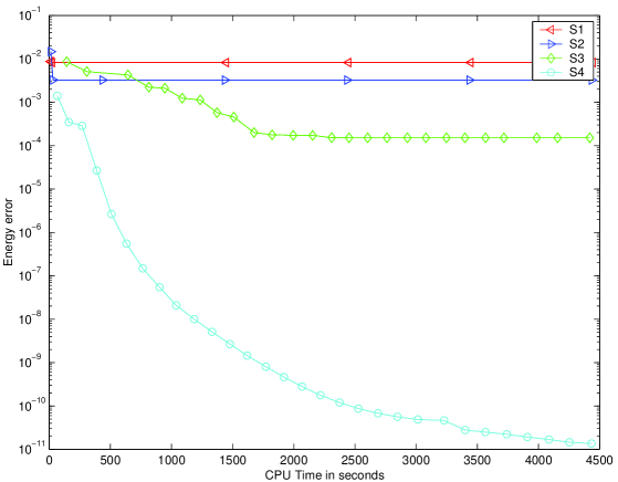
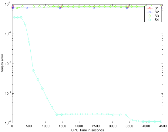
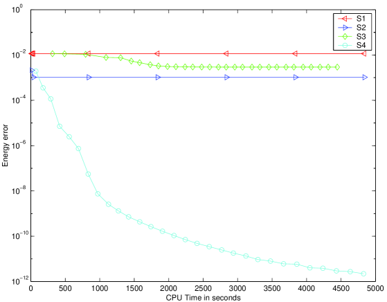
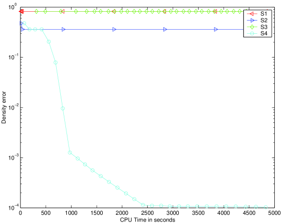
We compare the rate of convergence for the above four strategies. Two categories of tests are performed, depending on the quality of the initial guess. The results displayed on Figures 6 to  9 concern polymer $\mathcal{P}_{1}$ with $n_{m}=801$ monomers. This corresponds to $N_{b}=8050$ and $N=5622$. Analogous tests were performed on $\mathcal{P}_{2}$ and $\mathcal{P}_{3}$, but we do not present them here, for brevity.

The energy of the ground state of this matrix (i.e. the minimum of (1.6)) is $E_{0}=-27663.484$. The number of blocks considered is $p=100$. For the global step, we have collected these 100 blocks in $99$ overlapping groups of $2$ blocks. Interestingly, such a partition provides with optimal results regarding CPU time and memory requirement. It is observed on Fig. 6-9 that ${\mathcal{S}}_{1}$, ${\mathcal{S}}_{2}$ and ${\mathcal{S}}_{3}$ are not satisfactory for they converge towards some local, non global, minima of (2.2) whatever the initial guess. The failure of the strategy $S_{3}$ performed on the initial guess ${\mathcal{I}}_{2}$ is surprising: this initial guess is not good enough. Indeed, if the initial guess is ${\mathcal{I}}_{3}$, we check numerically that the strategies ${\mathcal{S}}_{3}$ and ${\mathcal{S}}_{4}$ behave identically. Notice that the strategy ${\mathcal{I}}_{3}$ is identical to ${\mathcal{S}}_{2}$ applied to the initial guess ${\mathcal{I}}_{2}$.

We also remark that the strategy ${\mathcal{S}}_{4}$ performs very well whatever the initial guess (see Fig. 7 and Fig. 9). The same behavior is observed for the polymers ${\mathcal{P}}_{2}$ and ${\mathcal{P}}_{3}$. Finally, after orthonormalization, the Density Matrix Minimization (DMM) method [18] failed with the random initial guess and reveals very slow with the initial guess ${\mathcal{I}}_{2}$. That is the reason why we consider the initial guess ${\mathcal{I}}_{3}$ to compare these methods.

4.3 Comparison with two other methods

Having emphasized the usefulness of all the ingredients of our MDD algorithm, we now compare it to two other algorithms:

• the diagonalization routine dsbgv.f from the LAPACK library;

• the Density Matrix Minimization (DMM) method [18].

These two algorithms are seen as prototypical approaches for standard diagonalization algorithms and linear scaling techniques respectively. They are only used here for comparison purposes. Regarding linear scaling methods, two other popular approaches are the Fermi Operator method [11] and the McWeeny iteration method [21]. We have observed that, at least in our own implementation, based on the literature, they are outperformed by the DMM method for the actual chemical systems we have considered. We therefore take DMM as a reference method for our comparison.

Recall that the routine dsbgv.f consists in the three-step procedure

• transform the generalized eigenvalue problem into a standard eigenvalue problem by applying a Cholesky factorization to $S$;

• reduce the new matrix to be diagonalized to a tridiagonal form;

• compute its eigenelements by using the implicit $QR$ method.

The algorithmic complexity of this approach is in $N_{b}^{3}$ and the required memory scales as $N_{b}^{2}$.

For the description of DMM method, we refer to [18]. Let us only mention here that this approach consists in a minimization procedure, applied to the energy expressed in terms of the density matrix. Both the algorithmic complexity and the memory needed for performing the DMM approach scale linearly with respect to the size $N_{b}$ of the matrix. The DMM method is initialized with the density matrix $D=CC^{t}$ computed with the initial guess $C$ of the domain decomposition method. Two important points for the tests shown below are the following.

First, we perform a cut-off on the coefficients on the various matrices manipulated throughout the calculation: only the terms of the density matrices within the frame defined in Figure 4 are taken into account. Such a cut-off has some impact on the qualities of the results obtained with the DMM method. We are however not able to design a better comparison.

Second, the DMM method requires the knowledge of the Fermi level (as is the case for the linear scaling methods commonly used in practice to date). The determination of the Fermi level is the purpose of an outer optimization loop. In contrast, the MDD approach computes an approximation of the Fermi level at each iteration. Here, for the purpose of comparison, we provide DMM with the exact value of the Fermi level. Consequently, the CPU times for the DMM method displayed in the sequel are underestimated.

We emphasize that the routine dsbgv.f computes the entire spectrum of the matrix, both eigenvalues and eigenvectors. In contrast, the MDD approach only provides with the lowest $N$ eigenvalues, among $N_{b}$, and the projector on the vector space spanned by the corresponding eigenvectors, not the eigenvectors themselves.

4.3.1 Comparison with Direct diagonalization and DMM

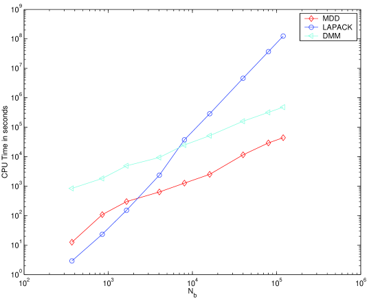
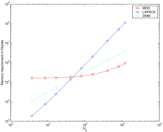
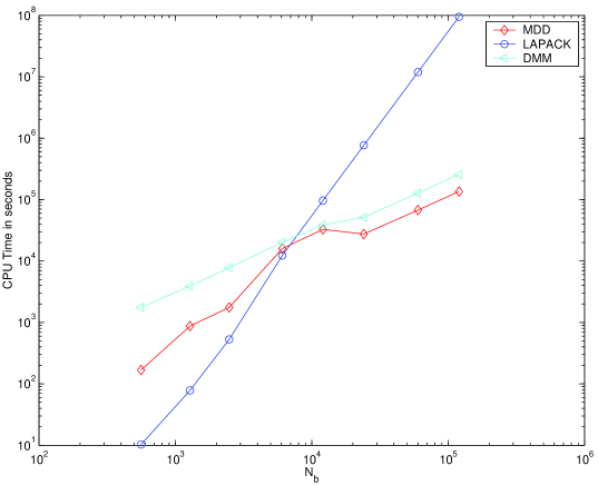
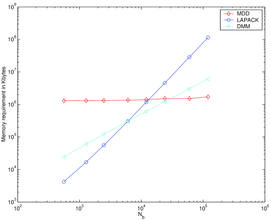
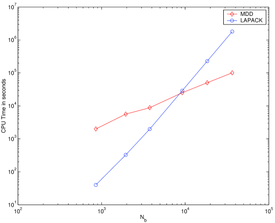
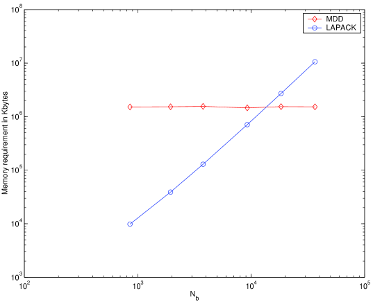
We have computed the ground states of the polymers ${\mathcal{P}}_{1}$, ${\mathcal{P}}_{2}$ and ${\mathcal{P}}_{3}$ with the three methods (direct diagonalization, DMM and MDD) and for various numbers $n_{m}$ of monomers, corresponding to matrix sizes $N_{b}$ in the range $10^{3}$-$10^{5}$.

For DMM and MDD, the initial guess is generated following the strategy ${\mathcal{I}}_{3}$. The results regarding the CPU time at convergence and the memory requirement are displayed on Figures 10 to 12 for the polymers $\mathcal{P}_{1}$, $\mathcal{P}_{2}$, and $\mathcal{P}_{3}$ respectively.

For small values of $N_{b}$, i.e. up to around $10^{4}$, the results observed for the direct diagonalization, DMM and MDD agree. The CPU times for our MDD approach scale linearly with $N_{b}$.

For larger values of $N_{b}$, the limited memory prevented us from either performing an exact diagonalization or from implementing DMM. So, we extrapolate the CPU time and memory requirement according to the scaling observed for smaller $N_{b}$.

The data for the DMM method are not plotted in Figure 12 as the DMM method does not converge for the polymer ${\mathcal{P}}_{3}$ when the number of monomers exceeds $10^{3}$. From our point of view, it comes from the truncation errors which cause the divergence of the method (note that the truncation strategy we consider here is very simple).

4.3.2 Comparison with DMM and a hybrid strategy

We now concentrate on the two approaches that scale linearly, namely DMM and MDD. We consider

• ${\mathcal{P}}_{1}$ with $4001$ monomers, corresponding to $N_{b}=40050$,

• ${\mathcal{P}}_{2}$ with $2404$ monomers, corresponding to $N_{b}=24080$,

• ${\mathcal{P}}_{3}$ with $208$ monomers, corresponding to $N_{b}=854$.

These particular values have been chosen for the purpose of having simple values for the numbers of blocks. For each of the three polymers, we compare the DMM and MDD methods initialized by the strategy ${\mathcal{I}}_{3}$ and a hybrid strategy. The hybrid strategy consists of a certain number of iterations performed with MDD, until convergence is reached for this method, followed by iterations with DMM. We use the following stopping criterion for MDD:

$$\|D_{n}-D_{n-1}\|\geq\|D_{n-1}-D_{n-2}\|\quad\mbox{{and}}\quad\|D_{n}-D_{n-1}\|\leq\epsilon_{a}$$ (4.2)

where $\epsilon_{a}$ is a threshold parameter. We take $\epsilon_{a}=10^{-4}$, respectively $\epsilon_{a}=10^{-3}$, for the polymer ${\mathcal{P}}_{1}$, respectively ${\mathcal{P}}_{2}$ and ${\mathcal{P}}_{3}$.

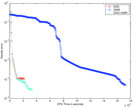
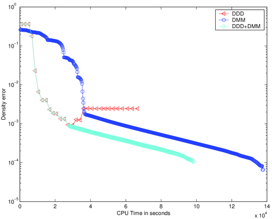
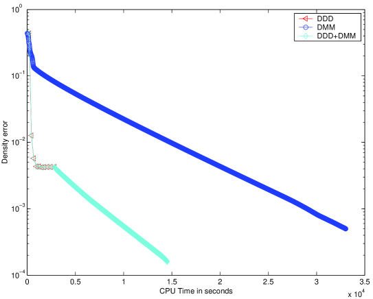
The Figures 13 to 15 show the evolution of the error in density versus CPU time. The hybrid version is demonstrated to be a very efficient combination of the two algorithms.

For completeness, let us highlight the temporary increase for the error in density appearing in Fig. 14 when MDD is used on $\mathcal{P}_{2}$. Analogously, the energy of the current solution, which is actually below the reference energy, also increases. In fact, this is due to a loss of precision in the orthonormality constraints. In MDD, these constraints are not imposed exactly at each iteration, but only approximately (see equation 3.12).

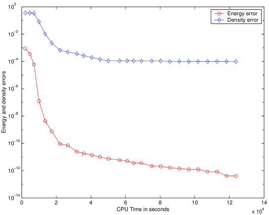
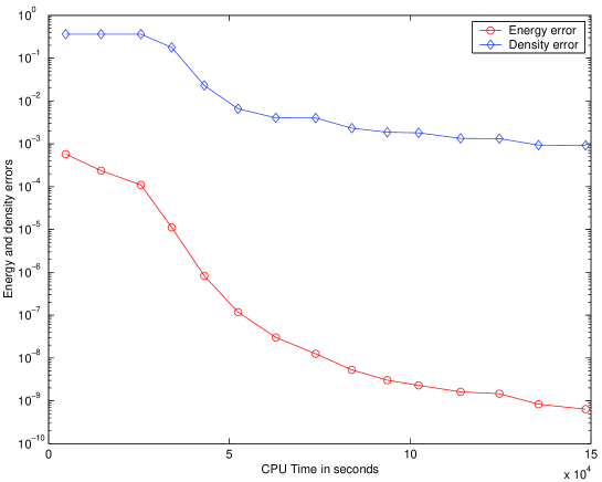
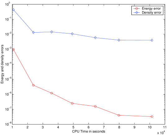
Finally, we report in figures 16 to 18 the results obtained with MDD for the largest possible case that can be perfomed on our platform, owing to memory limitation. We used the initial guesses obtained with the strategy ${\mathcal{I}}_{3}$. Notice that for the local step the memory requirement scales linearly with respect to the number $n_{m}$ of monomers, while for the global step, the memory requirement is independent of $n_{m}$. Therefore, for large polymers, the memory needed by MDD is controled by the local step. In contrast, for small polymers, the most demanding step in terms of memory is the global step.

5 Conclusions and remarks

The domain decomposition algorithm introduced above performs well, in comparison to the two standard methods considered. More importantly, our approach is an effective preconditionning technique for DMM iterations. Indeed, MDD provides a rapid and accurate approximation, both in terms of energy and density matrix, regardless of the quality of the initial guess. In contrast, DMM outperforms MDD when the initial guess is good, but only performs poorly, or may even diverge, when this is not the case. The combination of the two methods seems to be optimal. More generally, our MDD algorithm could constitute a good preconditionner to all variational methods, such as the Orbital Minimization method [20].

Regarding the comparison with DMM, the following comments are in order.

• All our calculations have been performed on a single processor machine. Potentially, both DMM and MDD should exhibit the same speed-up when parallelized. We therefore consider the comparison valid, at least qualitatively, for parallel implementations. The parallelization of the MDD is currently in progress, and hopefully will confirm the efficiency of the approach.

• We recall the Fermi level has to be provided to the DMM method. This is an additional argument in favor of the MDD approach.

• The MDD method, in contrast to the other linear scaling methods, does not perform any truncation in the computations. So, once the profile of $C$ is choosen, the method does not suffer of any instabilities, contrary to DMM (or OM) for which divergences have been observed for the polymer ${\mathcal{P}}_{3}$.

• The domain decomposition method makes use of several threshold parameters. For the three polymers we have considered, the optimal values of these parameters, except for the stopping criterion $\epsilon_{a}$ (equation (4.2)), are the same. We do not know yet if this interesting feature is a general rule.

• Recall our method solves problem (2.2), which is only an approximation of problem (2.1). Therefore, the relative error obtained in the limit is only a measure of the difference between (2.2) and (2.1). In principle, such a difference could be made arbitrarily small by an appropriate choice of the parameters of problem (2.2).

• Finally, let us emphasize that there is much room for improvement in both the local and the global steps. We have designed an overall multilevel strategy that performs well, but each subroutine may be significantly improved. Another interesting issue is the interplay between the nonlinear loop in the Hartree-Fock or Kohn-Sham problems (Self-Consistent Field - SCF - convergence [7, 8, 14]) and the linear subproblem considered in the present article. Future efforts will go in these directions.

Acknowledgments. We would like to thank Guy Bencteux (EDF) for valuable discussions and for his help in the implementation. C.L.B. and E.C. would like to acknowledge many stimulating discussions with Richard Lehoucq (Sandia National Laboratories).

Figure 1: Band structure of the symmetric matrix $H$.

Figure 2: Block structure of the matrices $C$. Note that by construction each block only overlaps with its nearest neighbors.

Figure 3: Block structure of the matrix $H$.

Figure 4: Block structure of the matrix $D$.

Figure 5: Collection of $p=10$ blocks into $r=3$ groups.

Figure 6: Energy error versus CPU time obtained with a bad initial guess (${\mathcal{I}}_{1}$).

Figure 7: Density error versus CPU time obtained with a bad initial guess (${\mathcal{I}}_{1}$).

Figure 8: Energy error versus CPU time obtained with a better initial guess (${\mathcal{I}}_{2}$).

Figure 9: Density error versus CPU time obtained with a better initial guess (${\mathcal{I}}_{2}$).

Figure 10: Scaling of the CPU time (top) and memory requirement (bottom) for the polymer ${\mathcal{P}}_{1}$.

Figure 11: Scaling of the CPU time (top) and memory requirement (bottom) for the polymer ${\mathcal{P}}_{2}$.

Figure 12: Scaling of the CPU time (top) and memory requirement (bottom) for the polymer ${\mathcal{P}}_{3}$.

Figure 13: Evolution of the density error with the CPU time for the polymer ${\mathcal{P}}_{1}$ made of $4001$ monomers.

Figure 14: Evolution of the density error with the CPU time for the polymer ${\mathcal{P}}_{2}$ made of $2404$ monomers.

Figure 15: Evolution of the density error with the CPU time for the polymer ${\mathcal{P}}_{3}$ made of $208$ monomers.

Figure 16: Evolution of the MDD energy and density errors versus CPU time for the polymer ${\mathcal{P}}_{1}$ ($20001$ monomers, $N_{b}=200050$).

Figure 17: Evolution of the MDD energy and density errors versus CPU time for the polymer ${\mathcal{P}}_{2}$ ($12004$ monomers, $N_{b}=120080$).

Figure 18: Evolution of the MDD energy and density errors versus CPU time for the polymer ${\mathcal{P}}_{3}$ ($5214$ monomers, $N_{b}=36526$).

References

- [1] E. Anderson, Z. Bai, C. Bischof, S. Blackford, J. Demmel, J. Dongarra, J. Du Croz, A. Greenbaum, S. Hammarling, A. McKenney and D. Sorensen, LAPACK users’ guide, 3rd edition, SIAM 1999.
- [2] P. Arbenz, U.L. Hetmaniuk, R.B. Lehoucq and R.S. Tuminaro, A comparison of eigensolvers for large-scale 3D modal analysis using AMG-preconditioned iterative methods, Int. J. Numer. Meth. Engng 64 (2005) 204-236.
- [3] D.A. Areshkin, O.A. Shenderova, J.D. Schall and D.W. Brenner, Convergence acceleration scheme for self consistent orthogonal basis set electronic structure methods, Mol. Sim. 29 (2003) 269-286.
- [4] N.W. Ashcroft and N. D. Mermin, Solid-State Physics, Saunders College Publishing 1976.
- [5] M. Barrault, Développement de méthodes rapides pour le calcul de structures électroniques, thèse de l’Ecole Nationale des Ponts et Chaussées, 2005.
- [6] D. Bowler, T. Miyazaki and M. Gillan, Recent progress in linear scaling ab initio electronic structure theories, J. Phys. Condens. Matter 14 (2002) 2781-2798.
- [7] E. Cancès, M. Defranceschi, W. Kutzelnigg, C. Le Bris, and Y. Maday, Computational Quantum Chemistry: a Primer, in: Handbook of Numerical Analysis, Special volume, Computational Chemistry, volume X, North-Holland 2003.
- [8] E. Cancès and C. Le Bris, Can we outperform the DIIS approach for electronic structure calculations, Int. J. Quantum Chem. 79 (2000) 82-90.
- [9] J.J.M. Cuppen, A divide and conquer method for symmetric tridiagonal eigenproblems, Numer. Math. 36 (1981) 177-195.
- [10] P.M.W. Gill, Molecular integrals over gaussian basis functions, Adv. Quantum Chem. 25 (1994) 141-205.
- [11] S. Goedecker, Linear scaling electronic structure methods, Rev. Mod. Phys. 71 (1999) 1085-1123.
- [12] W.J. Hehre, L. Radom, P.v.R. Schleyer, and J.A. Pople, Ab initio molecular orbital theory, Wiley 1986.
- [13] U.L. Hetmaniuk and R.B. Lehoucq, Multilevel methods for eigenspace computations in structural dynamics, Proceedings of the 16th International Conference on Domain Decomposition Methods, Courant Institute, New-York, January 12-15, 2005.
- [14] K.N. Kudin, G.E. Scuseria and E. Cancès, A black-box self-consistent field convergence algorithm: one step closer, J. Chem. Phys. 116 (2002) 8255-8261.
- [15] W. Kohn, Analytic properties of Bloch waves and Wannier functions, Phys. Rev. 115 (1959) 809-821.
- [16] W. Kohn, Density functional and density matrix method scaling linearly with the number of atoms, Phys. Rev. Lett. 76 (1996) 3168-3171.
- [17] C. Le Bris, Computational chemistry from the perspective of numerical analysis, Acta Numerica,volume 14, 2005, pp 363-444.
- [18] X.-P. Li, R.W. Numes and D. Vanderbilt, Density-matrix electronic structure method with linear system size scaling, Phys. Rev. B 47 (1993) 10891-10894.
- [19] R. McWeeny, Methods of molecular quantum mechanics, 2nd edition, Academic Press 1992.
- [20] P. Ordejón, D.A. Drabold, M.D. Grumbach and R.M. Martin, Unconstrained minimization approach for electronic computations that scales linearly with system size, Phys. Rev. B 48 (1993) 14646-14649.
- [21] A. Palser and D. Manopoulos, Canonical purification of the density matrix in electronic structure theory, Phys. Rev. B 58 (1998) 12704-12711.
- [22] Y. Saad, Numerical methods for large eigenvalue problem : theory and algorithms, Manchester University Press 1992.
- [23] D. Sánchez-Portal, P. Ordejón, E. Artacho and J.M. Soler, Density-functional method for very large systems with LCAO basis sets, Int. J. Quantum Chem. 65 (1997) 453-461.
- [24] W. Yang and T. Lee, A density-matrix divide-and-conquer approach for electronic structure calculations of large molecules, J. Chem. Phys. 163 (1995) 5674.
- [25] C. Paige and M. Saunders, Solution of sparse indefinite systems of linear equations, SIAM J. Numer. Anal., 12, 617-629, 1975.
- [26] M.J. Frisch, G.W. Trucks, H.B. Schlegel, G.E. Scuseria, M.A. Robb, J.R. Cheeseman, V.G. Zakrzewski, J.A. Montgomery, R.E. Stratmann, J.C. Burant, S. Dapprich, J.M. Millam, A.D. Daniels, K.N. Kudin, M.C. Strain, O. Farkas, J. Tomasi, V. Barone, M. Cossi, R. Cammi, B. Mennucci, C. Pomelli, C. Adamo, S. Clifford, J. Ochterski, G.A. Petersson, P.Y. Ayala, Q. Cui, K. Morokuma, D.K. Malick, A.D. Rabuck, K. Raghavachari, J.B. Foresman, J. Cioslowski, J.V. Ortiz, B.B. Stefanov, G. liu, A. Liashenko, P. Piskorz, I. Kpmaromi, G. Gomperts, R.L. Martin, D.J. Fox, T. Keith, M.A. Al-Laham, C.Y. Peng, A. Nanayakkara, C. Gonzalez, M. Challacombe, P.M.W. Gill, B.G. Johnson, W. Chen, M.W. Wong, J.L. Andres, M. Head-Gordon, E.S. Replogle and J.A. Pople, Gaussian 98 (Revision A.7), Gaussian Inc., Pittsburgh PA 1998.