Universal dynamics in the onset of a Hagen–Poiseuille flow

Abstract

The dynamics in the onset of a Hagen–Poiseuille flow of an incompressible liquid in a channel of circular cross section is well-studied theoretically. We use an eigenfunction expansion in a Hilbert space formalism to generalize the results to channels of arbitrary cross section. We find that the steady state is reached after a characteristic time scale $\tau=(\mathcal{A}/\mathcal{P})^{2}(1/\nu)$ where $\mathcal{A}$ and $\mathcal{P}$ are the cross-sectional area and perimeter, respectively, and $\nu$ is the kinematic viscosity of the liquid. For the initial dynamics of the flow rate $Q$ for $t\ll\tau$ we find a universal linear dependence, $Q(t)=Q_{\infty}\>(\alpha/\mathcal{C})\>(t/\tau)$, where $Q_{\infty}$ is the asymptotic steady-state flow rate, $\alpha$ is the geometrical correction factor, and $\mathcal{C}=\mathcal{P}^{2}/\mathcal{A}$ is the compactness parameter. For the long-time dynamics $Q(t)$ approaches $Q_{\infty}$ exponentially on the timescale $\tau$, but with a weakly geometry-dependent prefactor of order unity, determined by the lowest eigenvalue of the Helmholz equation.

I Introduction

Hagen–Poiseuille flow (or simply Poiseuille flow) is important to a variety of applications ranging from macroscopic pipes in chemical plants to the flow of blood in veins. However, the rapid development in the field of lab-on-a-chip systems during the past decade has put even more emphasis on pressure driven laminar flow. Traditionally, capillary tubes would have circular cross-sections, but today microfabricated channels come with a variety of shapes depending on the fabrication technique in use. The list of examples includes rectangular channels obtained by hot embossing in polymer wafers, semi-circular channels in isotropically etched surfaces, triangular channels in KOH-etched silicon crystals, Gaussian-shaped channels in laser-ablated polymer films, and elliptic channels in stretched PDMS devices, see e.g. Ref. Geschke:04a, .

This development has naturally led to more emphasis on theoretical studies of shape-dependence in microfluidic channels. Recently, we therefore revisited the problem of Poiseuille flow and its shape dependence and we have also addressed mass diffusion in microchannels Mortensen:05b ; Mortensen:05c . In the present work we combine the two former studies and address the dynamics caused by the abrupt onset of a pressure gradient at time $t=0$ in an incompressible liquid of viscosity $\eta$ and density $\rho$ situated in a long, straight, and rigid channel of length $L$ and some constant cross-sectional shape $\Omega$. The solution is well-known for the case of a cylindrical channel, see e.g. Ref. Batchelor:67, , but in this paper we generalize the results to a cross-section of arbitrary shape. The similarity between mass and momentum diffusion, and the existence of a characteristic diffusion time-scale $\tau_{\textrm{diff}}=(\pi/4)(\mathcal{A}/\mathcal{P})^{2}/D$ for mass diffusion Mortensen:05c have led us to introduce the momentum diffusion time-scale $\tau$ defined by

$$\tau=\Big{(}\frac{\mathcal{A}}{\mathcal{P}}\Big{)}^{2}\frac{1}{\nu},$$ (1)

where $\nu=\eta/\rho$ is the kinematic viscosity (having dimensions of a diffusion constant), while $\mathcal{A}$ and $\mathcal{P}$ is the area and perimeter of the cross section $\Omega$, respectively. In this paper we show that the dynamics of the flow rate $Q(t)$ is universal with $\tau$ as the characteristic time scale.

As shown in Ref. Mortensen:05b, the shape parameters $\mathcal{A}$ and $\mathcal{P}$ also play an important role in the steady-state Poiseuille flow. The hydraulic resistance $R_{\rm hyd}$ can be expressed as

$$R_{\rm hyd}=\alpha\>\frac{\eta L}{\mathcal{A}^{2}}\equiv\alpha R_{\rm hyd}^{*},$$ (2)

where $\alpha$ is a dimensionless geometrical correction factor and $R_{\rm hyd}^{*}=\eta L/\mathcal{A}^{2}$ is a characteristic resistance. Remarkably, $\alpha$ is simply (linearly) related to the dimensionless compactness parameter $\mathcal{C}=\mathcal{P}^{2}/\mathcal{A}$.

Above we have emphasized microfluidic flows because of the variety of shapes frequently encountered in lab-on-a-chip systems. However, our results are generally valid for laminar flows at any length scale.

II Diffusion of momentum

We consider a long, straight channel of length $L$, aligned with the $z$-axis, having a constant cross section $\Omega$ with the boundary $\partial\Omega$ in the $xy$ plane. The fluid flow is driven by a pressure gradient of $\boldsymbol{\nabla}p=-(\Delta p/L)\mathbf{e}_{x}$ which is turned on abruptly at time $t=0$. We note that strictly speaking the pressure gradient is not established instantaneously, but rather on a time-scale set by $L/c$ where $c$ is the speed of sound. For typical liquids $c\sim 10^{3}\,{\rm m/s}$ which for micro-fluidic systems and practical purposes makes the pressure gradient appear almost instantaneously. From the symmetry of the problem it follows that the velocity field is of the form $\mathbf{v}(\mathbf{r},t)=v(\mathbf{r}_{\perp},t)\mathbf{e}_{x}$ where $\mathbf{r}_{\perp}=y\mathbf{e}_{y}+z\mathbf{e}_{z}$. From the Navier–Stokes equation it then follows that $v(\mathbf{r}_{\perp},t)$ is governed by, see e.g. Refs. Batchelor:67, or Landau:87a, ,

$$\frac{1}{\nu}\>\partial_{t}v(\mathbf{r}_{\perp},t)-\nabla^{2}v(\mathbf{r}_{\perp},t)=\frac{\Delta p}{\eta L},$$ (3)

which is a diffusion equation for the momentum with the pressure drop acting as a source term on the right-hand side. The velocity $v$ is subject to a no-slip boundary condition on $\partial\Omega$ and obviously $v$ is initially zero, while it asymptotically approaches the steady-state velocity field $v_{\infty}(\mathbf{r}_{\perp})$ for $t\rightarrow\infty$.

In the analysis it is natural to write the velocity as a difference

$$v(\mathbf{r}_{\perp},t)=v_{\infty}(\mathbf{r}_{\perp})-v_{h}(\mathbf{r}_{\perp},t)$$ (4)

of the asymptotic, static field $v_{\infty}$, solving the Poiseuille problem

$$-\nabla^{2}v_{\infty}(\mathbf{r}_{\perp})=\frac{\Delta p}{\eta L},$$ (5)

and a time-dependent field $v_{h}(\mathbf{r}_{\perp},t)$ satisfying the homogeneous diffusion equation,

$$\frac{1}{\nu}\>\partial_{t}v_{h}(\mathbf{r}_{\perp},t)-\nabla^{2}v_{h}(\mathbf{r}_{\perp},t)=0.$$ (6)

From Ref. Mortensen:05c, it is known that rescaling the Helmholz equation by $(\mathcal{A}/\mathcal{P})^{2}$ leads to a lowest eigenvalue $a_{1}$ that is of order unity and only weakly geometry dependent. We therefore perform this rescaling, which naturally implies the time-scale $\tau$ of Eq. (1) and the following form of the diffusion equation,

$$\tau\>\partial_{t}v_{h}(\mathbf{r}_{\perp},t)-\hat{\mathscr{L}}v_{h}(\mathbf{r}_{\perp},t)=0.$$ (7)

where we have introduced the rescaled Laplacian $\hat{\mathscr{L}}$,

$$\hat{\mathscr{L}}\equiv\Big{(}\frac{\mathcal{A}}{\mathcal{P}}\Big{)}^{2}\nabla^{2}.$$ (8)

We note that by the rescaling the Navier–Stokes equation (3) becomes

$$\tau\>\partial_{t}v-\hat{\mathscr{L}}v=\Big{(}\frac{\mathcal{A}}{\mathcal{P}}\Big{)}^{2}\frac{\Delta p}{\eta L}=\frac{\alpha Q_{\infty}}{\mathcal{P}^{2}},$$ (9)

where we have introduced the steady-state flow rate $Q_{\infty}=\Delta p/R_{\textrm{hyd}}$ and used Eq. (2).

III Hilbert space formulation

In order to solve Eq. (9) we will take advantage of the Hilbert space formulation Morse:1953 , often employed in quantum mechanics Merzbacher:70 . The Hilbert space of real functions $f(\mathbf{r}_{\perp})$ is defined by the inner product

$$\big{<}f\big{|}g\big{>}\equiv\int_{\Omega}d\mathbf{r}_{\perp}\,f(\mathbf{r}_{\perp})g(\mathbf{r}_{\perp})$$ (10)

and a complete set $\big{\{}\big{|}\phi_{n}\big{>}\big{\}}$ of orthonormal basis functions,

$$\big{<}\phi_{m}\big{|}\phi_{n}\big{>}=\delta_{nm}.$$ (11)

Above, we have used the Dirac bra-ket notation and $\delta_{nm}$ is the Kronecker delta. We choose the eigenfunctions $\{\big{|}\phi_{n}\big{>}\}$ of the rescaled Helmholz equation (with a zero Dirichlet boundary condition on $\partial\Omega$) as our basis functions,

$$-\hat{\mathscr{L}}\big{|}\phi_{n}\big{>}=a_{n}\big{|}\phi_{n}\big{>}.$$ (12)

With this complete basis any function in the Hilbert space can be written as a linear combination of basis functions. Using the bra-ket notation Eq. (9) becomes

$$\tau\>\partial_{t}\big{|}v\big{>}-\hat{\mathscr{L}}\big{|}v\big{>}=\frac{\alpha Q_{\infty}}{\mathcal{P}^{2}}\big{|}1\big{>}.$$ (13)

The full solution Eq. (4) is written as

$$\big{|}v\big{>}=\big{|}v_{\infty}\big{>}-\big{|}v_{h}\big{>},$$ (14)

where $\big{|}v_{\infty}\big{>}$ satisfies the Poiseuille problem Eq. (5),

$$-\hat{\mathscr{L}}\big{|}v_{\infty}\big{>}=\frac{\alpha Q_{\infty}}{\mathcal{P}^{2}}\big{|}1\big{>},$$ (15)

and the homogeneous solution $\big{|}v_{h}\big{>}$ solves the diffusion problem Eq. (7)

$$\big{(}\tau\partial_{t}-\hat{\mathscr{L}}\big{)}\big{|}v_{h}\big{>}=0.$$ (16)

In the complete basis $\{\big{|}\phi_{n}\big{>}\}$ we have

$$\big{|}v_{h}\big{>} =\sum_{n=1}^{\infty}b_{n}e^{-a_{n}t/\tau}\big{|}\phi_{n}\big{>},$$ (17)

$$\big{|}v_{\infty}\big{>} =\sum_{n=1}^{\infty}c_{n}\big{|}\phi_{n}\big{>},$$ (18)

and since $\lim_{t\rightarrow 0}\big{|}v_{h}\big{>}=\big{|}v_{\infty}\big{>}$ we have $b_{n}=c_{n}$. Multiplying Eq. (18) by $\big{<}\phi_{m}\big{|}$ yields

$$b_{m}=c_{m} =\big{<}\phi_{m}\big{|}v_{\infty}\big{>}=\big{<}\phi_{m}\big{|}\hat{\mathscr{L}}^{-1}\hat{\mathscr{L}}\big{|}v_{\infty}\big{>}$$

$$=\frac{\alpha Q_{\infty}}{\mathcal{P}^{2}}\>a_{m}^{-1}\big{<}\phi_{m}\big{|}1\big{>}.$$ (19)

In the second-last equality we have introduced the unit operator $1=\hat{\mathscr{L}}^{-1}\hat{\mathscr{L}}$ and in the last equality we used the Hermitian property of the inverse Laplacian operator to let $\hat{\mathscr{L}}^{-1}$ act to the left, $\big{<}\phi_{m}\big{|}\hat{\mathscr{L}}^{-1}=-\big{<}\phi_{m}\big{|}a_{m}^{-1}$ from Eq. (12), while $\hat{\mathscr{L}}$ acts to the right, see Eq. (15). Substituting Eqs. (17) and (19) into Eq. (14) we finally obtain

$$\big{|}v\big{>}=\big{|}v_{\infty}\big{>}-\frac{\alpha Q_{\infty}}{\mathcal{P}^{2}}\sum_{n=1}^{\infty}\big{|}\phi_{n}\big{>}\big{<}\phi_{n}\big{|}1\big{>}\>a_{n}^{-1}e^{-a_{n}t/\tau}.$$ (20)

IV Flow rate

Using the bra-ket notation, the flow rate $Q(t)$ at any time is conveniently written as $Q=\big{<}1\big{|}v\big{>}$, and thus in steady state $Q_{\infty}=\big{<}1\big{|}v_{\infty}\big{>}$. Multiplying Eq. (20) from the left by $\big{<}1\big{|}$ yields

$$Q(t)=\big{<}1\big{|}v\big{>}=Q_{\infty}-\frac{\alpha Q_{\infty}}{\mathcal{P}^{2}}\sum_{n=1}^{\infty}\big{<}1\big{|}\phi_{n}\big{>}\big{<}\phi_{n}\big{|}1\big{>}\>a_{n}^{-1}e^{-a_{n}t/\tau}.$$ (21)

The factor $\big{<}1\big{|}\phi_{n}\big{>}\big{<}\phi_{n}\big{|}1\big{>}$ is recognized as the effective area $\mathcal{A}_{n}$ covered by the $n$th eigenfunction $\big{|}\phi_{n}\big{>}$,

$$\mathcal{A}_{n}\equiv\frac{\big{|}\big{<}1\big{|}\phi_{n}\big{>}\big{|}^{2}}{\big{<}\phi_{n}\big{|}\phi_{n}\big{>}}=\big{|}\big{<}1\big{|}\phi_{n}\big{>}\big{|}^{2}=\big{<}1\big{|}\phi_{n}\big{>}\big{<}\phi_{n}\big{|}1\big{>}.$$ (22)

The effective areas fulfil the sum-rule $\sum_{n=1}^{\infty}\mathcal{A}_{n}=\mathcal{A}$, seen by completeness of the basis $\big{\{}\big{|}\phi_{n}\big{>}\big{\}}$. We can find the geometrical correction factor $\alpha$ from Eq. (21) by using that $Q(0)=0$,

$$\alpha=\mathcal{P}^{2}\Bigg{(}\sum_{n=1}^{\infty}\frac{\mathcal{A}_{n}}{a_{n}}\Bigg{)}^{-1},$$ (23)

and substituting into Eq. (21) we finally get

$$\frac{Q(t)}{Q_{\infty}}=1-\Bigg{(}\sum_{n=1}^{\infty}\frac{\mathcal{A}_{n}}{a_{n}}\Bigg{)}^{-1}\sum_{n=1}^{\infty}\frac{\mathcal{A}_{n}}{a_{n}}\>e^{-a_{n}t/\tau}.$$ (24)

V Short-time dynamics

The short-time dynamics is found by Taylor-expanding Eq. (24) to first order,

$$\frac{Q(t)}{Q_{\infty}}\approx\Bigg{(}\sum_{n=1}^{\infty}\frac{\mathcal{A}_{n}}{a_{n}}\Bigg{)}^{-1}\mathcal{A}\>\frac{t}{\tau}=\frac{\alpha\mathcal{A}}{\mathcal{P}^{2}}\>\frac{t}{\tau}=\frac{\alpha}{\mathcal{C}}\>\frac{t}{\tau},\quad t\ll\tau,$$ (25)

where we have used the sum-rule for $\mathcal{A}_{n}$ as well as Eq. (23). The short time dynamics can also be inferred directly by integration of the Navier–Stokes equation Eq. (13), since at time $t=0$ we have $\big{|}v\big{>}=0$ and consequently the vanishing of velocity gradients and viscous friction, $\hat{\mathscr{L}}\big{|}v\big{>}=0$. Thus we arrive at

$$\tau\>\partial_{t}\big{|}v\big{>}=\frac{\alpha Q_{\infty}}{\mathcal{P}^{2}}\big{|}1\big{>},\quad t\rightarrow 0,$$ (26)

corresponding to a constant initial acceleration throughout the fluid. Integration with respect to $t$ is straightforward and multiplying the resulting $\big{|}v\big{>}$ by $\big{<}1\big{|}$ yields $Q(t)$,

$$\frac{Q(t)}{Q_{\infty}}\simeq\frac{\alpha}{\mathcal{P}^{2}}\big{<}1\big{|}1\big{>}\frac{t}{\tau}=\frac{\alpha\mathcal{A}}{\mathcal{P}^{2}}\frac{t}{\tau}=\frac{\alpha}{\mathcal{C}}\>\frac{t}{\tau},\quad t\ll\tau.$$ (27)

Thus initially, the fluid responds to the pressure gradient in the same way as a rigid body responds to a constant force.

shape	$a_{1}$	$\mathcal{A}_{1}/\mathcal{A}$	$\alpha/\mathcal{C}$
circle	$\gamma_{0,1}^{2}/4\simeq 1.45$a	$4/\gamma_{0,1}^{2}\simeq 0.69$a	2b
quarter-circle	1.27c	0.65c	1.85c
half-circle	1.38c	0.64c	1.97c
ellipse(1:2)	1.50c	0.67c	2.10c
ellipse(1:3)	1.54c	0.62c	2.21c
ellipse(1:4)	1.57c	0.58c	2.28c
triangle(1:1:1)	$\pi^{2}/9\simeq 1.10$d	$6/\pi^{2}\simeq 0.61$d	$5/3$b
triangle(1:1:$\sqrt{2}$)	$\frac{5\pi^{2}}{4(2+\sqrt{2})^{2}}\simeq 1.06$a	$512/9\pi^{4}\simeq 0.58$a	1.64c
square	$\pi^{2}/8\simeq 1.23$a	$64/\pi^{4}\simeq 0.66$a	1.78c
rectangle(1:2)	$5\pi^{2}/36\simeq 1.37$a	$64/\pi^{4}\simeq 0.66$a	1.94c
rectangle(1:3)	$5\pi^{2}/32\simeq 1.54$a	$64/\pi^{4}\simeq 0.66$a	2.14c
rectangle(1:4)	$17\pi^{2}/100\simeq 1.68$a	$64/\pi^{4}\simeq 0.66$a	2.28c
rectangle(1:$\infty$)	$\sim\pi^{2}/4\simeq 2.47$a	$64/\pi^{4}\simeq 0.66$a	$\sim 3$e
pentagon	1.30c	0.67c	1.84c
hexagon	1.34c	0.68c	1.88c

Table 1: Central parameters for the lowest eigenfunction for different cross sectional shapes. Note how the different numbers converge when going through the regular polygons starting from the triangle(1:1:1) through the square, the pentagon, and the hexagon to the circle. ^aSee e.g. Ref. Morse:1953, for the eigenmodes and eigenspectrum. Here, $\gamma_{0,1}$ denotes the first root of the zeroth Bessel function of the first kind. ^bSee Ref. Mortensen:05b, . ^cData obtained by finite-element simulations. ^dSee e.g. Ref. Brack:1997, for the eigenmodes and eigenspectrum. ^eSee e.g. Ref. Batchelor:67, for a solution of the Poisson equation.

VI Long-time dynamics

As the flow rate increases, friction sets in, and in the long-time limit $t\gg\tau$ the flow-rate saturates at the value $Q_{\infty}$ where there is a balance between the pressure gradient and frictional forces. For the long-time saturation dynamics the lowest eigenstate plays the dominating role and taking only the $n=1$ term in Eq. (24) we obtain

$$\frac{Q(t)}{Q_{\infty}}\simeq 1-e^{-a_{1}t/\tau},\quad t\gg\tau/a_{2},$$ (28)

where we have used that the lowest eigenvalue $a_{1}$ is non-degenerate to truncate the summation.

The time it takes to reach steady-state is denoted $\tau_{\infty}$. A lower bound $\tau_{1}$ for $\tau_{\infty}$ can be obtained from Eq. (27) by assuming that the initial acceleration is maintained until $Q(\tau_{1})/Q_{\infty}=1$ is reached,

$$\tau_{\infty}>\tau_{1}=\frac{\mathcal{C}}{\alpha}\>\tau.$$ (29)

A better estimate $\tau_{2}$ for $\tau_{\infty}$ is obtained from Eq. (28) by demanding $Q(\tau_{2})/Q_{\infty}=1-e^{-3}$.

$$\tau_{\infty}\approx\tau_{2}=\frac{3}{a_{1}}\>\tau.$$ (30)

Using the parameter values for the circle listed in Table 1 we find the values

$$\tau_{1}=0.5\>\tau<\tau_{2}=2.1\>\tau\approx\tau_{\infty}.$$ (31)

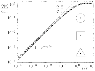
Figure 1: A log-log plot of the flow rate $Q(t)/Q_{\infty}$ as a function of time $t/\tau$. The dashed line is the short-time approximation Eq. (27), while the dashed-dotted line is the long-time approximation Eq. (28), both for the case of a circle, i.e., using $\mathcal{C}/\alpha=2$ and $a_{1}=1.45$ as listed in Table 1. The data points are the results of time-dependent finite-element simulations for the cases of the cross section being a circle (white circles), a square (gray squares), and an equilateral triangle (black triangles).

VII Numerical results

Only few geometries allow analytical solutions of both the Helmholz equation and the Poisson equation. The circle is of course the most well-known example, but the equilateral triangle is another exception. However, in general the equations have to be solved numerically, and for this purpose we have used the commercially available finite-element software Comsol 3.2 (see www.comsol.com). Numbers for a selection of geometries are tabulated in Table 1.

The circle is the most compact shape and consequently it has the largest value for $\mathcal{A}_{1}/\mathcal{A}$, i.e., the mode has the relatively largest spatial occupation of the total area. The eigenvalue $a_{1}$ is of the order unity for compact shapes and in general it tends to increase slightly with increasing values of $\mathcal{C}$. The modest variation from geometry to geometry in both $a_{1}$ and the other parameters suggests that the dynamics of $Q(t)$ will appear almost universal.

In order to illustrate the validity of our two asymptotic expressions, Eqs. (27) and (28), we have compared them using the values for a circular shape to time-dependent finite-element simulations of Eq. (3). As illustrated in Fig. 1 we find a perfect agreement between the asymptotic expressions Eqs. (27) and (28) and the numerically exact data for a circle, a square, and an equilateral triangle. Comparing the corresponding parameters in Table 1 we would expect all data to almost coincide, which is indeed also observed in Fig. 1. The small spread in eigenvalues and other parameters thus gives rise to close-to-universal dynamics. From the plot it is also clear that $\tau$ is indeed a good estimate for the time it takes to reach the steady state.

VIII Conclusions

In conclusion, by using a compact Hilbert space formalism we have shown how the initial dynamics in the onset of Poiseuille flow is governed by a universal linear raise in flow rate $Q(t)$ over a universal time-scale $\tau$ above which it saturates exponentially to the steady-state value $Q_{\infty}$. The steady state is reached after a time $\tau_{\infty}\approx{\mathcal{C}}\tau/\alpha$. Apart from being a fascinating example of universal dynamics for a complex problem our results may have important applications in design of real-time programmable pressure-driven micro-fluidic networks.

References

• (1) O. Geschke, H. Klank, and P. Telleman, editors, Microsystem Engineering of Lab-on-a-Chip Devices, Wiley-VCH Verlag, Weinheim, 2004.
• (2) N. A. Mortensen, F. Okkels, and H. Bruus, Phys. Rev. E 71, 057301 (2005).
• (3) N. A. Mortensen, F. Okkels, and H. Bruus, Phys. Rev. E 73, 012101 (2006).
• (4) G. K. Batchelor, An Introduction to Fluid Dynamics, Cambridge University Press, Cambridge, 1967.
• (5) L. D. Landau and E. M. Lifshitz, Fluid Mechanics, volume 6 of Landau and Lifshitz, Course of Theoretical Physics, Butterworth–Heinemann, Oxford, 2nd edition, 1987.
• (6) P. M. Morse and H. Feshbach, Methods of Theoretical Physics, McGraw–Hill, New York, 1953.
• (7) E. Merzbacher, Quantum Mechanics, Wiley & Sons, New York, 1970.
• (8) M. Brack and R. K. Bhaduri, Semiclassical Physics, Addison Wesley, New York, 1997.