Charges suspended by strings: A new twist to an old problem

1 Introduction

A popular problem [1] of calculating the equilibrium state in a system of two charged particles suspended on strings conventionally deals with mutually repelling charges (Fig.1, a). The students are typically asked to find the equilibrium separation $s$ between the charges or a related quantity such as the deflection angle. In this paper, we are slightly modifying this problem by considering two opposite and therefore attracting charges (Fig.1, b). Now, in order to generate an equilibrium state at finite distance $s$, we suspend the charges at a finite initial separation, rather than from the same point. One might expect that the problem with opposite charges is just a routine extension of the original one. It turns out however, that this is not case. The discussion leading to the solutions introduces a catastrophic behavior typically avoided in high school physics.

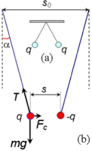
Figure 1: Equilibrium state of two charges suspended on strings. (a) illustrates the conventional problem with two identical charges (b) illustrates the modified problem with two opposite charges suspended at finite separation $s_{0}$ The corresponding force diagram is shown for $q>0$.

2 Problem

Two identical and oppositely charged    particles, $+q$ and $-q$, are suspended on two strings at an initial separation $s_{0.}$ The mass of each particle is $m$ and the length of the string is $l$. For simplicity, assume that $l\ >>s_{0}$ . This means that $\alpha$ can be treated as a small angle.

(A) Find how incrementing charge value $q$ starting from $q=0~{}$affecs the distance $s$ between the particles while neglecting the size of the particles. This is known as a point charge approximation.

(B) Now, view each particle as a point charge surrounded by an insulated hard spherical shell of radius $R$. How is the equilibrium relation $s(q)$ affected by R?

(C) Compare the ”forward” process (when $q$ is incremented from $q=0)$ with the ”reverse” (discharge) process when $q$ is decremented from the large values to $q=0$.

3 Solution

The equilibrium state of a system is defined by a force balance condition. There are three forces acting upon each charge: the linear tension of the string, $T$, the force of gravity mg (where $g$ is free acceleration) and the electrostatic force of attraction $F_{c}$. These forces are illustrated for one of the charges in Fig.1b. The electric force is determined by Coulomb’s law

$$F_{c}=k\frac{q^{2}}{s^{2}}$$ (1)

where $k$ is the electrostatic constant ($9\cdot 10^{9}\ N~{}m^{2}/C^{2})~{}$and $s$ is the separation between the charges. The condition that the net force vanishes results in the vector equation $\vec{T}+m\vec{g}+\vec{F}_{c}=0$. Splitting this into horizontal and vertical components yields the equations $T$sin($\alpha)=F_{c}$ and $T$ cos($\alpha)$ = mg Dividing the first by the second, we get:

$$\tan(\alpha)=\frac{F_{c}}{mg}$$ (2)

Formally this is identical to the equilibrium condition of the prototype problem [1]. However, if we now rewrite the equation in terms of the variable $s~{}$ features which are particular to our problem are revealed. To express $\tan(\alpha)$ through $s$, we notice that $\sin(\alpha)=(s-s_{0})/2l$.  Recalling that $\alpha$ is a small angle we may write $\tan(\alpha)\approx\sin(\alpha)=(s-s_{0})/2l$. Using this and Eq.1,  Eq.2 can be rewritten as

$$(s-s_{0})s^{2}=2k\frac{lq^{2}}{mg}$$ (3)

The problem can be solved generally in dimensionless units . However, since it is more traditional to use numerical examples for high school physics, further analysis we choose $l=1~{}$m$,~{}m=10^{-3}~{}$kg$,~{}s_{0}=0.2~{}$m. The other constants are $g=9.8$ m/s² and $k=9\cdot 10^{9}$ N m² /C².

Eq.3 completely describes the dependence $s(q)~{}$as requested in part A of the problem. However, the solution of this equation is not as trivial as for the prototype case. To illustrate how, we solve Eq.3 graphically by choosing different separations 0 $<s<s_{0}$ and determining the corresponding $q$ from the equation. A related problem along with a pedagogical justification of the graphical approach can be found in Can a Spring Beat the Charges? [2]

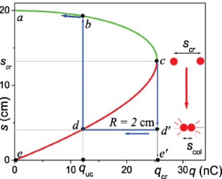
Figure 2: The green and red curves combine to form the plot of equilibrium distance dependence on charge, $s(q)$. The point where the two branches meet is labeled $c$ = ($q_{cr},s_{cr})$ and is termed the critical point. Note, $s$ is positioned along the vertical axis which is the conventional way of presenting $s(q)$ dependence. Points a-e and the interconnecting paths will be referenced in the discussion.

The solution is shown in Fig.2. We can now ask, what is the equilibrium separation for any given value of $q$ ? Surprisingly, for 0 $<$ q $<$ q_cr the graph gives two possible answers, represented by the green and red branches of the curve, while for $q$$>$$q_{cr}$ there are no solutions at all, i.e. $s(q)$ does not penetrate in that region. $q_{cr}$ denotes the boundary point between two regions where there is only one solution and s_cr is the corresponding separation. Which of two solutions found in the region $0<q<q_{cr}$ is “real”? In the next section it will be explained that these are the points on the green branch. The smaller equilibrium separations $s$$<$$s_{cr}$, i.e. the red branch, correspond to points of maxima of the underlying energy function and are therefore unattainable. We will also discover that this red branch becomes useful in the analysis of hysteresis (in answering the question C of the problem).

Let’s now examine the physical effects of varying the charge $q$ in closer detail. As charge $q$ grows from $0$ (the ”forward” process), the slope $s(q)$ becomes progressively steeper as demonstrated by the green curve. Finally, when $q$ approaches the critical value $q_{cr}\mathit{\sim 25.4}$ nC the slope of $s(q)$ becomes vertical (see $c$ in Fig.2).

What is the significance of this point for our system? At this critical point, the equilibrium disappears and the charges suddenly collapse. The distance between the charges changes instantly from $13.4$ cm (point $c)$ to 0 (point $e^{\prime})$.

The point charge approximation leads to a non-physical consequence. After the charges collapse, they stay intact attracted by an infinite force. The only way to separate them is to reduce $q$ to zero, and thereby entirely cancel the electrostatic attraction. While the point charge model is a useful approximation to get a grip on general qualitative behavior, in application to the collapsed state it becomes unrealistic.

Even the microscopic charges of interest, such as the ions or charged amino-acids in proteins, have finite size which prevents them from a complete collapse. To treat the collapsed state and the related behavior more realistically, we should assign finite sizes to our charges. We avoid some additional complications, such as discharge through contact, by assuming each charge is surrounded by a rigid insulating shell of finite radius R. This was the reasoning behind part B of the problem.

If the spheres have finite radii $R$, their closest possible separation is $2R$. Consequently, the length of the collapse in such a system decreases from $s_{cr}$ to $s_{cr}-2R$. As an example, the collapsed state for $R=2$ cm is represented in  Fig.2 by the blue line $d`d$separated from point $c$ by a vertical step = $13.4-4$ $=9.4~{}$cm. From this, one can see that for $R\geq s_{cr}/2$ the catastrophe disappears entirely because the shells prevent the system from entering the critical range. In such a case, increasing $q$ leads to continuous displacement of the charges until their surfaces come into contact. The described behavior is the answer to question B.

So far, we have approached the solution of the problem, but some questions remain unanswered. For instance, we still have to justify our neglect of the red curve and also explain the absence of equilibrium distances for $q>q_{cr}$. This will be done in the next section with the assistance of an energy function.

4 Energy and Stability

To understand the difference between the locally stable (green, upper branch in Fig.2) and unstable (red, lower branch) equilibrium states better, it is useful to analyze the energy profiles of the system. Given that the string is not stretchable, the potential energy $U$ of the system consists only of Coulombic and gravitational components. One can express the total potential energy as $U=2mgl~{}[1-\cos(\alpha)]-kq^{2}/s$.  Recalling that $\alpha$ is small and using the approximations $\cos(\alpha)\char 126\relax 1-\alpha^{2}/2~{}$and$\ \alpha\char 126\relax~{}\sin(\alpha)=(s-s_{0})/2l$, we get

$$U(s,q)=\frac{mg}{4l}(s-s_{0})-k\frac{q^{2}}{s}$$ (4)

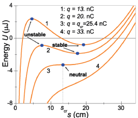
Figure 3: Energy profiles for different values of $q$.

Using the numeric values of the constants, and choosing representative values of $q$, we plot the energy profiles $U(s,q)$ in Fig.3. For $0~{}\mathit{<q<q}_{cr}$, $\mathit{U(s,q)}$ has a maximum at smaller $s$ and a minimum at larger $s$. The points of minima describe locally stable equilibrium states because small disturbances result in a restoring force. In contrast, maxima points are unstable because the system moves away from equilibrium after a small disturbance. This explains why the red branch was discarded in the preceding discussion.

For $q=q_{cr}$ both solutions merge forming the inflection point, also termed neutral equilibrium. The equilibrium disappears entirely for $q>q_{cr}$ because corresponding energy curves do not have a minima. (See curve 4 in Fig.3.) What is the cause of this anomaly? Let us note the different character of the forces. The horizontal component of tension varies almost linearly with $\alpha$ and correspondingly with $s$, whereas the Coulomb force is proportional to the inverse square of the separation $s$. The Coulomb force tends steeply to infinity as separation distance goes to 0. Consequently, for every $\mathit{q\neq 0}$ there exists a separation below which the Coulombic attraction will always overwhelm the counteracting tension force. This “equiforce” boundary separation coincides with the points of energy maxima and provides a physical interpretation of the red branch.

Also note, as $q$ grows, the region where the electric force overwhelms the horizontal tension widens until it engulfs the entire range at some value of $q$ which is exactly the point $q_{cr}$. Above that, the only possible equilibrium corresponds to the collapsed state. So it is this difference between the behaviors of the two forces that causes the catastrophe.

5 Irreversibility and Hysteresis

We still did not answer the question C of the problem. So far we have been assuming that $q$ was incremented starting from an initial value of 0 and separation $s_{0}$. But what if we reverse the process by starting from the collapsed state at charge value q $\geq$ q_cr, and then decremented $\mathit{q}$ to $\mathit{q=0}$? At what point would the charges separate?

This question has already been addressed for the case of point charges, where complete discharge is required for separation. We have also mentioned that when the shell radius $R$ $\geq s_{cr}/2$, the catastrophe and corresponding collapse disappear.

Thus, it only remains to consider radii $0$ $<$ $R$ $<s_{cr}/2$.  Let’s pick a representative value of $~{}R\prime=2~{}$cm and repeat the analysis of energy profiles familiar from the previous section. Note, the equilibrium separation in the collapsed state is no longer determined by the original condition $\overrightarrow{F}_{total}\ =\vec{T}+m\vec{g}+\vec{F}_{c}=0\$leading to Eq.3. Rather, the non-zero force $\overrightarrow{F}_{total}$ attracting the charges is balanced here by the repelling force due to rigidity of the shells.

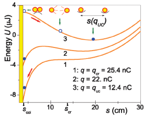
Figure 4: Presented are snapshots of energy profiles in three progressive stages of discharge. The plots are restricted to the accessible region s $\geq$ s_col . Initially, the system is in the collapsed state and at charge $q_{cr}$. The yellow bar represents the hard shell repulsion maintaining a lower bound on the separation distance at $s_{col}=2R\prime=4$ cm. Blue dot is the proverbial ball residing in a potential well. The cartoon depicts the uncollapse which happens when q approaches $q_{uc}$.

Consequently, the condition for separation is when the net attractive force $\overrightarrow{F}_{total}$ pressing the shells against each other vanishes. Obviously, this condition leads exactly to Eq.3. However, now it should be treated differently. Instead of finding an equilibrium separation for a fixed $q$, we use it to find a $q\$value for which the force at a fixed separation $s=2R~{}$vanishes.

For our example case of $s_{col}$ $=4\$ cm, the $q_{uc}$ determined by Eq.3 corresponds to the intersection point between the horizontal line $s=s_{col}$ and the curve $s(q)$ (see Fig. 2, point d ).

This result can be explained using the energy profiles in Fig. 4. Profile 1 corresponds to the collapsed state at $q=q_{cr}$. The attraction between the charges is compensated by contact repulsive force (see the yellow wall). The dip in the energy profile at distances close to $s_{col}$, creates an effective energy well which stabilizes the system.

Profile 2 illustrates how a decrease in the charge to $22$ nC makes the energy well trapping the system more shallow while still keeping the charges together.

Reducing $q$ further eventually leads to the scenario of profile 3. When $q_{uc}\sim 12.4$ nC is reached, the slope of the energy function at $s_{col}$ becomes horizontal. This means that the attractive force keeping the spheres together vanishes and the charge finds itself on the top of an energy hill. In other words, the equilibrium becomes unstable, so the charge rolls down to the stable energy well. This transition corresponds to the vertical line $d^{\prime}b~{}$connecting the red (maximum) and green (minimum) equilibrium positions in Fig.2. Since it is sudden, we term it an uncollapse . Fig.2 outlines the charging cycle for R = 2 cm with the path abcd’da. The vertical segment cd’ corresponds to the collapse, when separation suddenly changes from $13.4~{}$to $4$ cm. Additional charging will not change the separation. Decrementing $q$ after the collapse initially keeps the charges at fixed separation 4 cm, until $q_{ucl}\sim 12.4$ nC is reached (segment $d^{\prime}d)$. After that point, $s$ undergoes a vertical transition, an uncollapse, from the red to the green branch, db. Further decreases in $q$ will move charges apart along the green branch.

To extract a general principle from this example, we note that in the presence of catastrophe, the forward (charging) and reverse (discharging) behaviors are different. This irreversible behavior is called hysteresis. It is very common in many physical phenomena associated with instabilities, phase transitions and catastrophes.

6 Conclusion

The solution of the conventional problem of identical suspended charges $q$ describes a continuous relation between the equilibrium state and the value of $q$. Increasing $q$ leads to a monotonic increase of the deflection angle$\ \alpha$. For large values of $q$ the angle asymptotically approaches $\pi/2$ and the separation $s$ correspondingly approaches $2l$. Such behavior, when equilibrium properties smoothly depend on external parameters (pressure, charge, temperature, etc.) can be considered normal  [2] and is typical for practically all the equilibrium problems encountered in high school physics.

However, the real world is full of examples when smooth variation of external parameters results in sudden catastrophic change of equilibrium properties. The colloquialism, “the straw that broke the camel’s back”, expresses exactly this idea. These sorts of phenomena are directly related to physical catastrophes, instabilities and phase transitions.

As we can see, a generalization of the aforementioned problem for the case of opposite charges immediately results in catastrophic behavior. At a certain value of $q$ the equilibrium suddenly disappears, and system undergoes a sharp and discontinuous transition to a new equilibrium state. Usually, analysis of the catastrophic behavior requires very complex physics and mathematics. The discussion presented here and in references [2, 3] demonstrates that in some cases it can be accomplished with analytical tools available to high school physics students.

In this paper, we have also introduced the concept of hysteresis which is another feature of catastrophic behavior. It was shown that equilibrium separation between the charges for a given $q$ value can depend on charging history. We demonstrated that in some cases the same value of $q$, depending on how it was reached, can correspond either to a comparatively large separation or to a collapsed state where charges are stuck together. We believe guided investigation of the aforementioned phenomena can result in interesting student research projects.

References

- [1] D.C. Giancoli. Physics: Principles and applications. Prentice Hall, Upper Saddle River, NJ, 2 edition, 1997.
- [2] Michael B. Partensky and Peretz D. Partensky. Can a spring beat the charges? The Physics Teacher, pages 9–13, 2004.
- [3] Michael B. Partensky. Elastic capacitor and its unusual properties. http//oai:arXiv.org:physics/0208048, 2002.