Observation of a Turbulence–Induced Large Scale Magnetic Field

Abstract

An axisymmetric magnetic field is applied to a spherical, turbulent flow of liquid sodium. An induced magnetic dipole moment is measured which cannot be generated by the interaction of the axisymmetric mean flow with the applied field, indicating the presence of a turbulent electromotive force. It is shown that the induced dipole moment should vanish for any axisymmetric laminar flow. Also observed is the production of toroidal magnetic field from applied poloidal magnetic field (the $\omega$–effect). Its potential role in the production of the induced dipole is discussed.

Many stars and planets generate their own nearly–axisymmetric magnetic fields. Understanding the mechanism by which these fields are generated is a problem of fundamental importance to astrophysics. These dynamos are sometimes modeled using two components: a process which generates toroidal magnetic field from poloidal field and a feedback mechanism which reinforces the poloidal field Parker (1955). The first process is easily modeled in an axisymmetric system: toroidal differential rotation of a highly–conducting fluid sweeps the pre-existing poloidal field in the toroidal direction creating toroidal field. This phenomenon, known as the $\omega$–effect, is efficient at producing magnetic field and has been observed experimentally Lehnert (1957); Odier et al. (1998); Bourgoin et al. (2002). The second ingredient to the model is more subtle, as toroidal currents must be generated to reinforce the original axisymmetric poloidal field. Cowling’s theorem Cowling (1933) excludes the possibility of an axisymmetric flow generating such currents so some symmetry–breaking mechanism is required.

The usual mechanism invoked Moffatt (1978) is a turbulent electromotive force (EMF), $\cal{E}=\left<\tilde{\mathbf{v}}\times\tilde{\mathbf{b}}\right>$, whereby small scale fluctuations in the velocity and magnetic fields break the symmetry and interact coherently to generate the large scale magnetic field. This EMF is sometimes expanded Krause and Rädler (1980) in terms of transport coefficients about the mean magnetic field: $\cal{E}=\alpha\mathbf{B}+\beta\nabla\times\mathbf{B}+\bm{\gamma}\times\mathbf{B}$; $\alpha$ is characterized by helicity in the turbulence, $\beta$ by enhanced diffusion and $\bm{\gamma}$ by a gradient in the intensity of the turbulence. $\alpha$ is of particular interest as it results in current flowing parallel to a magnetic field, and when coupled with the $\omega$–effect can generate the toroidal currents needed to reinforce the poloidal field.

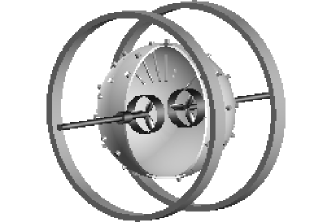
Figure 1: Schematic of the Madison Dynamo Experiment showing a cut-away view of the sphere, impellers, external field coils, surface and internal Hall probes.

Experimental evidence for mean–field EMFs (such as the $\alpha$–effect) in turbulent flows has been scarce. Three experiments, relying on a laminar $\alpha$–effect, have generated an EMF Steenbeck et al. (1968) and dynamo action Gailitis et al. (2000); Stieglitz and Müller (2001), but heavily-constrained flow geometries were used to produce the needed helicity; the role of turbulence was ambiguous. Experiments with unconstrained flows have provided evidence for turbulent EMFs, though not the turbulent $\alpha$–effect. Reighard and Brown Reighard and Brown (2001) have attributed a measured reduction in the conductivity of a turbulent flow of sodium to the $\beta$–effect. Pétrélis et al. have observed Pétrélis et al. (2003) distortion of a magnetic field similar to an $\alpha$–effect (currents generated in the direction of an applied magnetic field) and postulate that turbulence may be responsible for disagreement between a laminar model and observations. Not all liquid–metal experiments have had such results: Frick et al. have reported Frick et al. (2004) that the mean flow accounts for all magnetic fields in their torus–shaped gallium experiment, and Peffley, Cawthorne and Lathrop Peffley et al. (2000) have observed no such effects. It should also be noted that an $\alpha$–effect has been observed in the core of magnetically–confined plasmas Ji et al. (1996); Redd et al. (2002).

In this Letter we report measurements of the magnetic field induced by applying an axisymmetric magnetic field to a turbulent, axisymmetric flow of liquid sodium. An induced dipole moment is measured which cannot be generated by the mean flow, indicating the presence of a turbulent EMF.

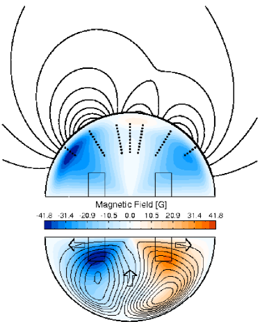
Figure 2: Upper half: color contours of induced toroidal magnetic field, $B_{\phi}(s,z)$, measured by sets of internal Hall probes, for $Rm_{tip}=100$. Induced poloidal flux surfaces, $\Psi(s,z)$, are in black. The positions of the internal Hall probes are indicated with dots. The cylindrical axis of symmetry is horizontal. Lower half: velocity field measured in a water model of the Madison Dynamo Experiment, for an impeller rotation rate of 16.7 Hz. Contours of toroidal flow, $v_{\phi}(s,z)$, are in color and poloidal stream function, $\Phi(s,z)$, are in black. The arrows indicate the direction of the poloidal flow, and the rectangles indicate the positions and size of the impellers which drive the flow.

The study is conducted in the Madison Dynamo Experiment, a 1 m diameter stainless steel sphere containing liquid sodium. As shown in Fig. 1, two drive shafts enter the sphere through each pole and drive 30.5 cm diameter impellers which generate an axisymmetric mean flow. The shafts are coupled to two 75 kW motors which are independently controlled by variable–frequency drives. The radial component of the magnetic field is measured by an array of 74 temperature–compensated Hall probes mounted to the sphere’s surface, allowing resolution of spherical harmonic components of the external magnetic field up to polar order of $\ell=7$ and azimuthal order of $m=5$. Magnetic fields within the sphere are measured by seven linear arrays of Hall probes inserted into the sodium within stainless steel sheaths. These probes are oriented to measure either the axial or toroidal component of the field. Finally, two external electromagnets, in a Helmoltz configuration coaxial with the impellers, apply a nearly uniform magnetic field throughout the sphere. The applied field is between 0 and 60 G, and dominated by spherical harmonic content of $\ell=1,m=0$; the largest measured $m\neq 0$ component of the applied field is less than 2% of the axisymmetric part.

The study is conducted in the kinematic regime—the magnetic field is not strong enough to affect the flow. The strength of the Lorentz force relative to the inertial forces acting on the fluid is characterized by the interaction parameter (also called the Stuart number), $N=\sigma aB_{0}^{2}/\rho v_{0}$, where $a$ is the radius of the sphere, $\sigma$ and $\rho$ are the conductivity and density of the fluid, respectively, and $B_{0}$ and $v_{0}$ are characteristic magnetic and velocity field magnitudes. $N\sim 10^{-2}$ for a total magnetic field of 100 G and $v_{0}=16.0$ m/s, so the magnetic field is not expected to alter the flow. This is confirmed by the linear dependence of the induced magnetic field with respect to the applied field. To affect the flow we would expect $N\approx 0.1$, or $B_{0}\approx 180$ G, a field magnitude not yet achieved. We note that the fluctuations, which are characterized by slower velocities, may be in a regime that is affected by the magnetic field.

The axisymmetric part of the velocity field generated by the impellors can be expressed in cylindrical coordinates $(s,\phi,z)$ as

$$\mathbf{v}=\nabla\Phi\times\nabla\phi+v_{\phi}(s,z)\hat{\bm{\phi}},$$ (1)

where $\Phi(s,z)$ is the poloidal stream function. The flow consists of two large cells, one in the northern and one in the southern hemisphere. An example of this flow, based on measurements made in a water model of the sodium apparatus Forest et al. (2002), can be seen in the lower half of Fig. 2. The poloidal cells flow inward at the equator and outward at the poles. The two toroidal cells flow in opposing directions. The flow is similar to the $t2s2$ flow proposed by Dudley and James Dudley and James (1989); a flow which is calculated to magnetically self-excite at sufficiently high magnetic Reynolds number, $Rm=\mu_{0}\sigma av_{0}$, where $\mu_{0}$ is the vacuum magnetic permeability ($Rm_{tip}=\mu_{0}\sigma av_{tip}$, where $v_{tip}$ is the impeller tip speed). This study is conducted below the critical $Rm$ for self-excitation, as demonstrated by the lack of observed growing magnetic fields. The Reynolds number of the fluid is $Re\sim 10^{7}$; turbulent fluctuations of the measured flow can be as large as 20% of the mean, depending on location.

Once the sphere is full of sodium the motors are started and a constant magnetic field is applied to the sphere. Hall probes sample the magnetic field at 1 kHz for 5 minutes; the applied field is then subtracted from these data to determine the induced field. Measurements of the induced field are presented in the upper half of Fig. 2. The field is represented by a toroidal component, $B_{\phi}(s,z)$, and poloidal flux function, $\Psi(s,z)$, such that

$$\mathbf{B}=\nabla\Psi\times\nabla\phi+B_{\phi}(s,z)\hat{\bm{\phi}}.$$ (2)

The toroidal magnetic field, undetectable by probes outside the sphere and orthogonal to the applied poloidal field, is measured within the sphere by internal Hall probes, confirming the presence of the $\omega$–effect. The peak amplitude of the toroidal magnetic field scales linearly with $Rm$, and can be larger than the magnitude of the applied field.

The external induced poloidal magnetic field is decomposed into its spherical harmonic components to reveal its spatial structure. Since the Hall probes on the sphere’s surface lie outside regions containing currents the magnetic field can be expressed as the gradient of a scalar magnetic potential, $\mathbf{B}=-\nabla\Phi_{m}$, which solves Laplace’s equation. In spherical coordinates the solution to the potential, for the region excluding the origin, is well known: $\Phi_{m}(r,\theta,\phi)=\sum_{\ell,m}D_{\ell,m}r^{-(\ell+1)}Y_{\ell}^{m}(\theta,\phi)$, where $Y_{\ell}^{m}(\theta,\phi)$ is the spherical harmonic. The coefficients in the expansion, $D_{\ell,m}$, which fit the mean induced field are calculated using singular value decomposition. The induced poloidal magnetic field is predominantly axisymmetric; the largest components are given in Tab. 1. The dominant components with $\ell$ equal to 3 and 5 are expected due to the structure of the applied field and mean flow; the large measured dipole component is not expected, as it cannot be generated by the axisymmetric mean flow, as will be shown below.

Harmonic ($\ell$, $m$)	Energy	$B_{r,max}$	RMS Fluctuation
$1,\,0\,({\rm dipole})$	$1.6\;{\rm erg}$	$11.4\,{\rm G}$	$1.8\,{\rm G}$
$2,\,0$	$0.2$	$3.1$	$3.5$
$3,\,0$	$0.5$	$13.6$	$2.4$
$4,\,0$	$0.1$	$7.1$	$3.5$
$5,\,0$	$0.4$	$18.3$	$3.5$
$1,\,1$	$0.0$	$0.8$	$7.8$
$2,\,1$	$0.0$	$0.6$	$3.3$

Table 1: Mean energy in the largest induced external poloidal harmonics, maximum mean radial field on the sphere’s surface, and field fluctuation level for several spherical harmonic components, for $Rm_{tip}=100$ and an applied field of 60 G.

Figure 3: Induced dipole moment versus time, for $Rm_{tip}=100$ and an applied magnetic field of 60 G. 1 G m³ corresponds to 13.2 G at the sphere’s pole.

The induced dipole moment fluctuates dramatically in time around a well–defined mean, as seen in Fig. 3. Measurements indicate that the induced dipole depends on $Rm$ (Fig. 4a) and upon the magnitude of the externally–applied field (Fig. 4b). The dipole moment’s dependence on $Rm$ eliminates the possibility of the measurement being a systematic error in the analysis. The EMF depends linearly on the applied field, indicating that it is a kinematic effect and not due to the back reaction.

Figure 4: (a) Mean induced dipole moment versus $Rm_{tip}$, for an applied field of 60 G with a quadratic fit valid at low $Rm$. (b) Mean induced dipole moment versus applied magnetic field, for $Rm_{tip}=100$. A linear fit is plotted for comparison. Error bars are RMS fluctuation levels about the mean; the uncertainties in the mean values are very small (less than 0.01 G m³) due to long averaging times.

While Cowling’s theorem demonstrates that self-excitation is not possible in axisymmetric systems, it is not obvious that a dipole moment cannot be induced by an axisymmetric velocity field exposed to an axisymmetric magnetic field. The proof of this is as follows. Consider a bounded, steady–state, axisymmetric system described by Eq. 2. For axisymmetric fields, the only non-trivial component of the dipole moment, $\bm{\mu}\equiv\int\mathbf{x}\times\mathbf{J}\,d^{3}x$, is oriented along the symmetry axis and results from currents flowing in the toroidal direction,

$$\mu_{z}=\int sJ_{\phi}\,d^{3}x.$$ (3)

These currents can only be generated by the $\mathbf{v}\times\mathbf{B}$ force due to the mean fields, so using Ohm’s law gives

$$sJ_{\phi} = s\sigma\left[\mathbf{v}\times\left(\nabla\Psi\times\nabla\phi\right)\right]\cdot\hat{\bm{\phi}}$$ (4)

$$= \sigma\left[v_{\phi}\nabla\Psi-\left(\mathbf{v}\cdot\nabla\Psi\right)\hat{\bm{\phi}}\right]\cdot\hat{\bm{\phi}}$$

$$= -\sigma\nabla\cdot\left(\mathbf{v}\Psi\right),$$

where use has been made of $\nabla\Psi\cdot\hat{\bm{\phi}}=0$ and the fluid has been assumed incompressible, $\nabla\cdot\mathbf{v}=0$. Inserting Eq. 4 into Eq. 3 and making use of Gauss’ theorem and $\mathbf{v}\cdot\hat{\bm{n}}=0$, where $\hat{\bm{n}}$ is the unit vector normal to the vessel’s surface, one finds that $\mu_{z}=0$. It is interesting to note that it is only the dipole moment that vanishes; moments which include different powers of $s$ in Eq. 3 are nonzero in general. This conclusion is also independent of geometry; any simply–connected axisymmetric system gives the same result.

It is possible that an induced dipole could be generated if mean non-axisymmetric magnetic and velocity field modes interacted. The stainless steel tubes which contain the internal Hall probes could potentially break the symmetry and create a mean non-axisymmetric flow. However, if this were the case one would expect higher–order non-axisymmetric induced field components, which are not observed (see Tab. 1). The mean induced dipole moment is present both with and without the tubes.

Since it cannot be generated by the mean flow, the dipole moment must be the result of turbulence breaking the symmetry of the system, likely a turbulent EMF of some form. Any of the terms in the mean–field expansion of the EMF have the potential to yield the observed mean dipole moment. A toroidal $\alpha$–effect could produce large scale toroidal currents by interacting with the observed $\omega$–effect. The small scale helicity needed for the $\alpha$–effect might come from either a turbulent cascade or be produced directly by the impellers. The $\beta$–effect leads to turbulent modifications of the fluid conductivity Krause and Rädler (1980). A nonuniform $\beta$–effect could cause uneven distributions of currents to generate the dipole moment. A third possibility is the $\gamma$–effect Krause and Rädler (1980), which expels magnetic field from regions of high–intensity turbulence, resulting in diamagnetism. The intensity of the turbulence varies with position, so the $\beta$–effect and the $\gamma$–effect are both candidates to explain the field.

Expanding the EMF in terms of the mean magnetic field may not be appropriate, since the largest fluctuations in the magnetic field do not satisfy the scale–separation and homogeneity requirements usually imposed in the expansion of the mean–field EMF. The largest turbulent magnetic fluctuations are $m=1$. Their Gaussian probability distribution is centered at zero, consistent with a passively–advected magnetic field in a turbulent cascade of velocity fluctuations. These $m=1$ fluctuations in $\mathbf{B}$ could, in principle, interact with $m=1$ fluctuations in the flow and average to give a net toroidal current.

In summary, a mean dipole moment is induced in the experiment which cannot be produced by the mean flow. The induced currents are of the correct form to create a poloidal magnetic field, as required in the $\alpha\omega$–dynamo model Parker (1955). This is the first observation of this effect in a laboratory experiment. Explicit characterization of the EMF is impossible without more detailed knowledge of the form of the turbulence and direct measurement of the fluctuating components of $\mathbf{v}$ and $\mathbf{B}$. Future work will be directed towards identifying the characteristics of the fluctuations responsible for producing the dipole field. We also note that no saturation of the mechanism has yet been definitively observed, as might be expected from numerical simulations and theory Gruzinov and Diamond (1994); Cattaneo and Hughes (1996). Future experiments with larger magnetic fields may provide insight into the saturation mechanism.

We express our gratitude to A. Bayliss for helpful dialogue and C. Parada for assistance with data acquisition. CBF would like to thank S. Prager and P. Terry for their continued support and useful discussions. This work is funded by the US Department of Energy, the National Science Foundation, and David and Lucille Packard Foundation.

References

- (1)
- Parker (1955) E. N. Parker, Astrophys. J. 122, 293 (1955).
- Lehnert (1957) B. Lehnert, Ark. Fys. 13, 109 (1957).
- Odier et al. (1998) P. Odier, J.-F. Pinton, and S. Fauve, Phys. Rev. E 58, 7397 (1998).
- Bourgoin et al. (2002) M. Bourgoin et al., Phys. Fluids 14, 3046 (2002).
- Cowling (1933) T. G. Cowling, Mon. Not. R. Astron. Soc. 94, 39 (1933).
- Moffatt (1978) H. K. Moffatt, Magnetic field generation in electrically conducting fluids (Cambridge University Press, 1978).
- Krause and Rädler (1980) K. Krause and K. H. Rädler, Mean-field Magnetohydrodynamics and Dynamo Theory (Pergammon Press, 1980).
- Steenbeck et al. (1968) M. Steenbeck, I. M. Kirko, A. Gailitis, A. P. Klyavinya, F. Krause, I. Y. Laumanis, and O. A. Lielausis, Sov. Phys.–Doklady 13, 443 (1968).
- Gailitis et al. (2000) A. Gailitis et al., Phys. Rev. Lett. 84, 4365 (2000).
- Stieglitz and Müller (2001) R. Stieglitz and U. Müller, Phys. Fluids 13, 561 (2001).
- Reighard and Brown (2001) A. Reighard and M. Brown, Phys. Rev. Lett. 86, 2794 (2001).
- Pétrélis et al. (2003) F. Pétrélis, M. Bourgoin, L. Marié, J. Burguete, A. Chiffaudel, F. Daviaud, S. Fauve, P. Odier, and J.-F. Pinton, Phys. Rev. Lett. 90 (2003).
- Frick et al. (2004) P. Frick, S. Denisov, S. Khripchenko, V. Noskov, D. Sokoloff, R. Stepanov, and R. Volk, in MHD Couette Flows: Experiments and Models, edited by R. Rosner, G. Rüdiger, and A. Bonanno (American Institute of Physics, 2004), vol. 733 of AIP Conference Proceedings, pp. 58–67.
- Peffley et al. (2000) M. Peffley, A. Cawthorne, and D. Lathrop, Phys. Rev. E 61, 5287 (2000).
- Ji et al. (1996) H. Ji, S. Prager, A. Almagri, J. Sarff, Y. Yagi, Y. Hirano, K. Hattori, and H. Toyama, Phys. Plasmas 3, 1935 (1996).
- Redd et al. (2002) A. Redd, B. Nelson, T. Jarboe, P. Gu, R. Raman, R. Smith, and K. McCollam, Phys. Plasmas 9, 2006 (2002).
- Forest et al. (2002) C. Forest, R. Bayliss, R. Kendrick, M. Nornberg, R. O’Connell, and E. Spence, Magnetohydrodynamics 38, 107 (2002).
- Dudley and James (1989) M. L. Dudley and R. W. James, Proc. R. Soc. London, Ser. A 425, 407 (1989).
- Gruzinov and Diamond (1994) A. Gruzinov and P. Diamond, Phys. Rev. Lett. 72, 1651 (1994).
- Cattaneo and Hughes (1996) F. Cattaneo and D. W. Hughes, Phys. Rev. E 54, 4532 (1996).