Coexistence of single–mode and multi–longitudinal mode emission in the ring laser model
Abstract
A homogeneously broadened unidirectonal ring laser can emit in several longitudinal modes for large enough pump and cavity length because of Rabi splitting induced gain. This is the so called Risken-Nummedal–Graham-Haken (RNGH) instability. We investigate numerically the properties of the multi–mode solution. We show that this solution can coexist with the single–mode one, and its stability domain can extend to pump values smaller than the critical pump of the RNGH instability. Morevoer, we show that the multi–mode solution for large pump values is affected by two different instabilities: a pitchfork bifurcation, which preserves phase–locking, and a Hopf bifurcation, which destroys it.
keywords:
Laser instabilities , Self–pulsing , BistabilityPACS:
42.60.Mi , 42.65.Sf, , ,
The Risken-Nummedal–Graham-Haken (RNGH) instability was first described in two independent papers in 1968 [1, 2]. In short, the instability consists in the destabilization of single longitudinal–mode emission, which appears immediately above the lasing threshold in a single transverse–mode homogeneously–broadened unidirectional ring laser, in favor of multilongitudinal mode emission. The physical mechanism responsible for that instability is the Rabi splitting of the lasing transition, induced by the lasing mode, which leads to the appearance of gain for the sideband modes [3, 4, 5].
After the instability, the laser emits in a pulsing regime because of the beating between different longitudinal modes, which are phase–locked. It is to be emphasized that no inhomogeneity, nor spectral nor spatial, is needed for multi–mode emission. For a recent review of the RNGH instability, see [6] and references therein.
Although some analytical work can be done regarding what happens after the instability occurs, it is evident that the multi–mode emission regime needs to be analyzed numerically. The situation is similar to that of the Lorenz–Haken (LH) instability, which is the single–mode counterpart of the RNGH instability. However, while the dynamics associated with the LH instability has been completely and since a long time characterized through a large number of numerical studies [7, 8], a lot of work has still to be done to achieve the same degree of knowledge for the RNGH instability.
The first numerical study about the dynamics associated with the RNGH instability was carried out by Risken and Nummedal themselves [9] but since then, along almost forty years, only a few works have been devoted to that [3, 10, 11, 12, 13, 14]. It must also be noted that some of these studies are quite superficial as they were intended to show some examples of the pulsing regime rather than characterizing it.
An important aspect of the RNGH instability is the supercritical or subcritical character of the bifurcation. We remind that if the pump parameter is the control parameter and is the pump value at which the single–mode solution destabilizes (also known as the second laser threshold), the bifurcation is supercritical if the multi–mode solution that arises from the instability exists only for , and it is subcritical if it exists also for . In the latter case, the multi–mode solution will coexist with the stable single–mode solution in the interval , where must be in general determined numerically. This region of the parameter space is called hard excitation domain, because within that domain a large perturbation of the stable single–mode solution allows to make the transition to the multi–mode solution.
The understanding of this question may be important for the correct interpretation of the experimental results recently obtained in erbium–doped fiber lasers (EDFLs) [15, 16, 17, 18] (see also [6]). In fact, if the bifurcation is subcritical the self–pulsing regime may be observed experimentally for pump values smaller than the instability threshold given by the linear stability analysis of the single–mode solution, and the transition from cw emission to self–pulsing would be discontinuous.
For the RNGH instability the instability domain is usually represented in the plane, where is the properly scaled side–mode frequency. The instability domain has the shape of a tongue delimited by the curves and , which merge at the critical point (see Fig. 1). is the critical frequency at which the instability threshold attains its minimum value . The single–mode solution is unstable if, for a given pump , there is at least one side–mode whose frequency lies inside the tongue.

A number of numerical and analytical studies have shown that the multi–mode solution exists not only inside the instability domain, but also for and , where the linear stability analysis predicts stable single–mode emission.
This result was found numerically already by Risken and Nummedal in their second paper of 1968 [9]. They showed that, fixing and decreasing from an initial value larger than , the single–mode solution bifurcates to the multi–mode solution at and this solution persists even when the other boundary is crossed. Risken and Nummedal were not able to determine the lower boundary of the existence domain of the multi–mode solution, because the numerical analysis of that solution is problematic for small . In fact, as decreases the pulses becomes higher and narrower and in order to reproduce them correctly a very small spatial stepsize is needed, which implies increasing computation time.
Later on, Haken and Ohno [19, 20, 21] derived a generalized Ginzburg–Landau equation for the critical (unstable) mode and found again the coexistence of the two solutions, which are the minima of an effective potential. They also showed that the transition from single–mode to multi–mode emission can be supercritical or subcritical depending on the frequency , but they did not write an analytic expression of this result.
Simpler analytic results can be found considering some particular limits for the parameters and , where , and are the decay rates of electric field, medium polarization and population inversion.
In the limit of class–B lasers (), for which , Fu [22] derived analytically an unambiguous condition: If the pump parameter is the bifurcation parameter, the bifurcation is supercritical (subcritical) when (). This result has been recently generalized for conditions outside the uniform field limit [6]. The same result was found by Carr and Erneux in a slightly different limit for class–B lasers () [23].
All these results mean that multi–mode emission can be found for parameter settings for which the single–mode solution is still stable. Nevertheless, the minimum instability threshold pump has been always found to be a lower bound for multi–mode emission. In general, the condition that determines sub– or supercritical bifurcation is not known, and it remains to be determined whether the multi–mode solution can exist not only for , but also for outside the class–B limit.
In this paper we address this question and show that, outside the class B–limit, the multi–mode solution can indeed exist for although not below the limit . Moreover, we perform an accurate study of the multi–mode solution and show that, increasing the pump power for a fixed frequency , the solution is affected by two instabilities in sequence. The first is a pitchfork instability, which breaks the symmetry of the solution, but preserves phase–locking. The second is a Hopf instability, which unlock the phases, introducing a slow modulation of the pulses.
In Section 2 we introduce the model equations and recall the main results concerning the RNGH instability, in Section 3 we illustrate and comment the numerical results and finally in Section 4 we draw our conclusions.
1 Model
Consider an incoherently pumped and homogeneously broadened two–level active medium of length , contained in a ring cavity of length , interacting with a unidirectional plane wave laser field. We assume that the cavity is resonant with the atomic transition frequency and that the cavity mirrors reflectivities are close to unity so that the uniform field limit holds. The Maxwell–Bloch equations describing such a laser can be written in the form [6]
| (1) | |||||
| (2) | |||||
| (3) |
In these equations is the normalized slowly varying envelope of the laser field and and are the normalized slowly varying envelope of the medium polarization and the population inversion, respectively (see [6] for the normalizations). The parameters , and have been already defined in the Introduction. We use the adimensional time and longitudinal coordinate , which are related with time and space through and , where
| (4) |
is the adimensional free spectral range of the cavity, being the light velocity in the host medium. The actual free spectral range of the cavity, FSR, is related to by
| (5) |
hence represents the FSR measured in units of the homogeneous linewidth. The boundary condition for the electric field
| (6) |
means that can be expressed as a superposition of plane waves with a spatial wave–number equal to an integer multiple of (with our scaling of space and time denotes both the spatial wave–number and the temporal frequency).
Eqs. (1-3) have two stationary solutions, the laser–off solution and , and the resonant single–mode lasing solution , and , where is an arbitrary phase. This solution appears at the lasing threshold .
The linear stability analysis of the single–mode solution has been reported many times, see e.g., [6]. This solution is unstable for a given if with
| (7) | |||||
| (8) | |||||
| (9) |
These equations give the bifurcation line on the plane. The instability occurs for a minimum pump when and where
and can be obtained from Eqs. (7) and (8) setting and . In Fig. 1, we represent the instability boundary on the plane for and .
2 Numerical results
We have numerically integrated Eqs. (1-3) for fixed relaxation rates and , letting the frequency and the pump as variable parameters. Notice that, although , this choice of the parameters does not mean that we are considering a class–A laser, i.e. a laser where the time evolution of electric field is much slower than those of the material variables. This would be true in the single–mode limit, but here we are studying a multi–mode laser, where the –th side–mode oscillates at an angular frequency of order 1 or larger, therefore the time scale of the electric field is comparable to those of the material variables, as in class–C lasers.
Our choice of corresponds to a mirror transmissivity close to 0.1. In fact, if distributed losses are negligible, the cavity linewidth and the free spectral range are related by , and we will consider values of around 4.
The integration method is based on a modal expansion of the electric field [14]
| (10) |
which allows to convert Eqs. (1-3) into a set of ordinary integro–differential equations for the complex mode amplitudes and for the variables and , with . For the present analysis we verified that 11 modes () and a spatial grid of points are enough to reproduce accurately the total electric field.
We proceeded as follows: First we fixed between and and took a pump value for which the single–mode solution is unstable. Then we varied the pump in both directions to determine the boundaries of the multi–mode solution. We repeated the operation for several values of even moving below . In Fig. 2 the boundary of multi–mode emission found in this way is represented with a dashed–dotted line together with the boundary of the single–mode solution instability domain, indicated by the solid line. The shadowed area marks the domain where both the single–mode and the multi–mode solutions are stable.
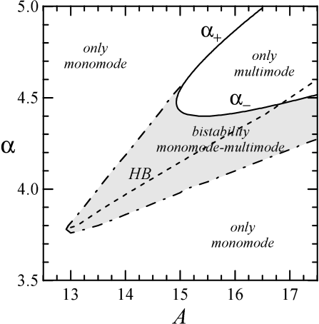
Two features of the bistability domain are of particular
interest:
(i)
The domain extends to the left up to , well below .
(ii) The domain extends up to a frequency larger than . Hence, considering
as the bifurcation parameter, the bifurcation is subcritical not
only for , as shown by Fu
in the class–B limit, but also for
.
(iii) The domain extends
up to a minimum frequency .
Let us now characterize the multi–mode dynamics existing in the range of parameters covered in Fig. 2. There are two clearly different regimes that are separated by the dashed line that crosses the bistability regime (marked as ). At the left of the dashed line, multi–mode emission is periodic, the modal intensities are constant and phases are locked. The dashed line marks a Hopf bifurcation. At the right of this line the dynamics of the total intensity is quasi–periodic and the modal intensities and the relative phases oscillate periodically in time.
In order to analyze this in more detail, we describe now the dynamics of the system for the particular value as a function of the pump parameter . In Fig. 3 the modal intensities corresponding to the central mode, , and the two first sidebands (modes and ) are represented as a function of (the intensities of higher order modes are, at least, one order of magnitude smaller than ).

There are three clearly distinguishable zones in Fig.
3:
(i) For , the modal
intensities are constant and single–valued, and symmetric modes
have the same intensity (,
).
(ii) for , the modal
intensities are constant but there are two possible solutions,
denoted as and in the figure, and symmetric
modes have different intensities (). Precisely,
when , then , and
viceversa.
(iii) For the modal intensities are
no more constant (for this domain, in the figure we have
represented the extrema of the modal intensities).
Hence, looking at the modal intensities, we can conclude that they are subject to a pitchfork, symmetry breaking, bifurcation at and to a Hopf bifurcation at .
We studied more in detail the two multi–mode self–pulsing solutions that coexist in the interval . One could imagine that these solutions differ in the total intensity, because all the modes placed on one side of the spectrum have intensities larger than the corresponding modes on the other side. But this is not the case: the shape of the pulses emitted by the laser is exactly the same for the two solutions. How this can be possible can be understood looking at the behavior of modal frequencies and phases.
In the upper panel of Fig. 4 we show the calculated frequencies of the central mode and of the first side–modes , to which we have subtracted the empty cavity frequencies . In the lower panel of the same figure we represent in radians the relative phase , where is the phase of the –th mode. If the solution is phase–locked , as well as all the other relative phases that can be defined in the same way, must be constant.


We see that at the pitchfork bifurcation the modal frequencies experience a shift in the same direction, positive or negative for the two solutions. This shift however preserves phase–locking, although is no longer equal to 0 as for , but it can take two opposite values, associated with the two solutions. Notice that the maximum frequency separation between the two phase–locked solution is about 0.02.
The combination of different mode intensities, frequencies and relative phases makes it possible that the total intensities for the two solutions are identical.
Let us now analyze the laser dynamics beyond the Hopf bifurcation . In Figs. 5, 6, and 7 we considered the three different values for the pump , and . In each figure the upper panel shows the total intensity, the middle panel the modal intensities of the central mode and of the first two side–modes, and the lower panel the relative phase defined above, measured in radians. The total intensity displays a slow modulation with period of some hundreds time units, superimposed to the much faster self–pulsing oscillations of period . This slow modulation is clearly related to the oscillations of the modal intensities and of the relative phase, which have the same period. The period is almost the same in Figs. 5 and 6, and it is almost twice larger in Fig. 7. The strength of the modulation increases with , and the relative phase passes from the almost regularly periodic oscillations of Fig. 5(c) to the behavior shown in Fig. 7(c), where remains most of the time close to 0.
We notice that the slow modulation frequency for the smaller values of is close to the maximum frequency separation between the two phase–locked solutions that is achieved immediately before . Hence, we may interpret the dynamical state that arises from the Hopf bifurcation as a state where the two phase–locked solutions are present simultaneously, and oscillate at their beat note.
Let us finally comment that we have not found chaotic behavior. Certainly the quasi–periodic dynamics of the total intensity is more involved as pump increases, but multi–mode emission disappears before more complex dynamics develops.
3 Conclusion
We have numerically and theoretically investigated bistability between single–mode and multi–longitudinal mode solutions in the standard ring–cavity two–level laser within the uniform field limit. We have determined the domain of coexistence between the single–mode and multi–longitudinal mode solutions for a class–C laser (we have used , and ) finding that this domain is relatively wide. In particular we have found that the domain of coexistence is different from that corresponding to a class–B laser as it extends for slightly larger than and for (for class–B lasers it exists for and [22, 23]). We have also found that the multimode solution undergoes a pitchfork bifurcation (which is a symmetry breaking bifurcation) and a subsequent Hopf bifurcation that destroys mode–locking. In the near future we plan to extend this numerical study to a situation closer to that of the experimental conditions in [18], in order to determine up to what extent the deviations from the theoretial predictions could be interpreted as a manifestation of the coexistence between single–mode and multi–longitudinal mode emission.
We gratefully acknowledge G.J. de Valcárcel for continued discussions. This work has been supported by the Spanish Ministerio de Ciencia y Tecnología and European Union FEDER (Fonds Européen de Développpement Régional) through Project PB2002-04369-C04-01.
References
- [1] H. Risken and K. Nummedal, Phys. Lett. 26A (1968) 275.
- [2] R. Graham and H. Haken, Z. Phys. 213 (1968) 420.
- [3] K. Ikeda, K. Otsuka, and K. Matsumoto, Prog. Theor. Phys. Suppl. 99 (1989) 295.
- [4] C. O. Weiss and R. Vilaseca, Dynamics of Lasers, (VCH Verlagsgesellschaft, Weinheim, 1991).
- [5] Ya. I. Khanin, Priciples of Laser Dynamics, (Elsevier Science B.V., Amsterdam, 1995).
- [6] E. Roldán, G.J. de Valcárcel, F. Prati, F. Mitschke, and T. Voigt, Multilongitudinal mode emission in ring cavity class B lasers, in Trends in Spatiotemporal Dynamics in Lasers. Instabilities, Polarization Dynamics, and Spatial Structures, edited by O.G. Calderon and J.M. Guerra (Research Signpost, Trivandrum, India, 2005), pp. 1–80; also at arXiv:physics/0412071
- [7] C.T. Sparrow, The Lorenz equations: bifurcations, chaos and strange attractors, (Springer–Verlag, Berlin, 1982).
- [8] L.M. Narducci, H. Sadiki, L.A. Lugiato and N.B. Abraham, Opt. Commun. 55 (1985) 370.
- [9] H. Risken and K. Nummedal, J. Appl. Phys. 39 (1968) 4662.
- [10] M. Mayr, H. Risken, and H. D. Vollmer, Opt. Commun. 36 (1981) 480.
- [11] J. Zorell, Opt. Commun. 38 (1981) 127.
- [12] L. A. Lugiato, L. M. Narducci, E. V. Eschenazi, D. K. Bandy, and N. B. Abraham, Phys. Rev. A 32 (1985) 1563.
- [13] D. Casini, G. D’Alessandro, and A. Politi, Phys. Rev. A 55 (1997) 751.
- [14] G. J. de Valcárcel, E. Roldán, and F. Prati, J. Opt. Soc. Am. B 20 (2003) 825.
- [15] F. Fontana, M. Begotti, E. M. Pessina, and L. A. Lugiato, Opt. Commun. 114 (1995) 89.
- [16] E. M. Pessina, G. Bonfrate, F. Fontana, and L. A. Lugiato, Phys. Rev. A 56 (1997) 4086.
- [17] T. Voigt, M. O. Lenz, and F. Mitschke, Risken-Nummedal-Graham-Haken instability finally confirmed experimentally, in International Seminar on Novel Trends in Nonlinear Laser Spectroscopy and High–Precission Measurements in Optics, S. N. Bagaev, V. N. Zadkov, and S. M. Arakelian eds., Proc. SPIE 4429 (2001) 112.
- [18] T. Voigt, M. Lenz, F. Mitschke, E. Roldán, and G. J. de Valcárcel, Appl. Phys. B 79 (2004) 175.
- [19] H. Haken and H. Ohno, Opt. Commun. 16 (1976) 205.
- [20] H. Ohno and H. Haken, Phys. Lett. 59A (1976) 261.
- [21] H. Haken and H. Ohno, Opt. Commun. 26 (1978) 117.
- [22] H. Fu, Phys. Rev. A 40 (1989) 1868.
- [23] T. W. Carr and T. Erneux, Phys. Rev. A 50 (1994) 724.